Abstract—Early Convergence, input feature space with minimal dimensions and good classification accuracy are always the most desired characteristics of an unsupervised neural network based pattern classifier. To achieve these, various approaches comprising of various soft computing tools can be used at different levels of implementations of such classifiers. Rough set is also one such tool, which can be used at either preprocessing level or learning level or architectural implementation level. Approaches using rough sets at first and the third levels are discussed here. Use of rough sets at the above stated levels result in dimensionality reduction of feature space through preprocessing and early convergence through rough neuron.
Index Terms—Pattern classification, Reducts, Rough Neuron, Rough Sets, Unsupervised neural network,
I. INTRODUCTION
The philosophy of soft computing is to exploit the tolerance for imprecision, uncertainty by devising methods of computation, which lead to an acceptable solution at low cost. The principle constituents of soft computing i.e. Fuzzy logic, Neurocomputing, Genetic Algorithms and Rough sets are complementary rather than competitive. This paper focuses on the hybridization using rough sets and neural computing for pattern recognition. Rough sets and neural networks provide an efficient method for uncertainty and ambiguity handling. Rough set also has inherent capacity of handling consistent, inconsistent as well as incomplete type of data.
The paper explores the use of theory of rough sets in the stages of preprocessing and in architectural implementation of an unsupervised artificial neural network using Kohonen learning rule. The preprocessing stage involves the selection of features, which help in discerning classes by the evaluation of subjective probabilities. The reduced attributes set then forms the input to the unsupervised ANN composed of rough neurons. The rough neuron as introduced by Lingras [1] consists of the lower boundary and upper boundary
Submitted for International Conference on Soft Computing and Applications (ICSCA'08)
Ashwin kothari is Sr. Lecturer in department of Electronics and Computer Science, V.N.I.T, Nagpur, M.S. India-440010, Member IAENG. (Phone: +91 9890164705, +91 712 2801049; fax: 91 712 2223230; e-mail:
[email protected], [email protected] ).
Dr. Avinash Keskar is Prof. and Dean R&D in department of Electronics and Computer Science, V.N.I.T, Nagpur, M.S. India-440010. (e-mail:
Shreesha Srinath and Rakesh Chalsani are eighth semester B.Tech students of department of Electronics and Computer Science, V.N.I.T, Nagpur, M.S. India-440010. (e-mail: [email protected],
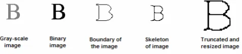
[image:1.595.307.545.181.234.2]Figure 1 Output at various preprocessing stages.
neurons. The input signal is split into lower boundary neuron signal, consisting of the more significant attributes present in the reduced set and the upper boundary neuron signal, containing the entire reduced set of attributes. Such an approach results in early convergence of the network, dimensionality reduction and improved classification accuracy.
II. PREPROCESSING STAGE
In case of large-scale inconsistency, rough sets are the most effective tools of approximation. Exploiting this inconsistency, rough sets can directly be used for finding out the discernibility between the input attributes to be fed to the neural classifier. For this case the needed information system is generated by a large database of samples consisting of images of printed alphabetical characters of 18 different fonts.
A. Image Preprocessing
The original data set is subjected to a number of preliminary processing steps to make it usable by the feature extraction algorithm. Pre-processing aims at producing data that is easy for the pattern recognition system to operate on accurately. The main objectives of pre-processing are: binarization, noise reduction, skeletonization, boundary extraction, stroke width compensation, truncation of redundant portion of image and resizing it to a specific size. In the end, the image is resized to a pre-defined size of 64 pixels x 64 pixels as shown figure 1.
B. Feature extraction
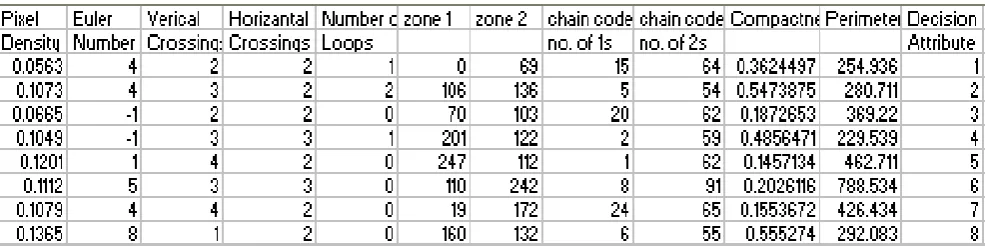
In feature extraction stage, each character is represented as a feature vector, which becomes its identity. The major goal of feature extraction is to extract a set of features, which maximizes the recognition rate with the least amount of elements. Total 31 features are extracted and are mainly of either structural or statistical type and help in obtaining local characteristics than the global ones. Thus some features contribute towards consistent part and the others contribute towards inconsistent part of the information system. The information system, of which is shown in figure 2, thus contains values with continuous intervals and hence has to
Rough Set Approach to Unsupervised Neural
Network based Pattern Classifier
undergo the process of discretization.
Figure 2 Sample information system
C. Discretization
The solution to deal with continuous valued attributes is to partition numeric variables into a number of intervals and treat each such interval as a category. This process of partitioning continuous variables is usually termed as discretization. Data can be reduced and simplified through discretization. In case of continuous valued attributes, large number of objects are generated with a very few objects mapping into each of these classes. The worst case would be when each value creates equivalence with only one object mapping into it. The discretization in rough set theory has particular characteristics, which should not weaken the indiscernibility ability. Although a variety of discretization methods have been developed and out of those, the most suitable method for the presented case is explained in [2].
III. FEATURE SPACE DIMENSIONALITY REDUTION Application of methods of dimensionality reduction to data analysis or pattern recognition problems has distinct advantages in terms of generalization properties and processing speed. For a large input system, besides the memory requirement, the processing time has to be addressed as well. Generally for larger systems, the processing time and the memory requirements increase significantly. One can reduce the memory requirement and processing time, by reducing, (i) the dimensions of the input data, or (ii) the number of input patterns (training patterns). The aim of dimensional reduction is to describe the input patterns by means of a minimum number of features, which are effective in discriminating between different classes. The objective of the preprocessing stage is to reduce the input dimensionality of the neural network without significantly affecting the features of the original set by selecting only the significant features. Also as described earlier, out of the various possible levels of using rough set based approaches; this level is the preprocessing level.
Fundamental principle of a rough set-based learning system is to discover redundancies and dependencies between the given features of a data to be classified. Rough set theory is efficient in uncertainty handling (upper and lower approximation of data points) and granular computing (using the objects in the information of the systems). Based on the above, following four subjective probabilities have been used to obtain the reduced set of significant features.
A. Method 1
In this method the relative significance of each attribute in discerning between two compared classes x & y is as given by:
,
( )
x y|
iP x
a
(1)Where P(x) x,y|ai is the probability of an object belonging to class x given the only information as attribute ai (
i=1,2,3,...,m) when discerning the objects of x from y. If the value turns out to be 1, then the particular attribute is most significant and if the value turns out to be 0, then the particular attribute is the least significant.
B. Method 2
In this method the relative significance of each attribute in discerning between two compared classes x & y is as given by:
,
( ( ))
i x y|
iP a x
a
(2)Where P(ai(x)) x,y|ai is the probability of the attribute value
ai(x) which will discern class x from y, given the only information as attribute ai ( i=1,2,3,...,m).
C. Method 3 & 4
In these methods the relative significance of each attribute in discerning two compared classes x & y is as given below:
, ,
( )
x y|
i( ( ))
i x y|
iP x
a P a x
+a
(3)
, * ,
( )
x y|
i( ( ))
i x y|
iP x
a P a x
a
(4)Where the terms P(x) x,y|ai & P(ai(x)) x,y|ai are explained as above.
D. Algorithm
Step 1: Obtain the information system for feature space dimensionality reduction.
Step 2: The matrix (t×t) is constructed and entry for each attribute is given by either of methods 1or 2 or 3 or 4., where t is number of decision attributes or the output classes in which the input data set is to be classified. (t is 26 in this case.).
Step 3: The relative sum for each attribute is obtained i.e. the contribution of each attribute over the table is summed up.
Step 4: The most significant contributors based on the relative sum are selected according to the requirement or the set threshold.
discussed in the results section.
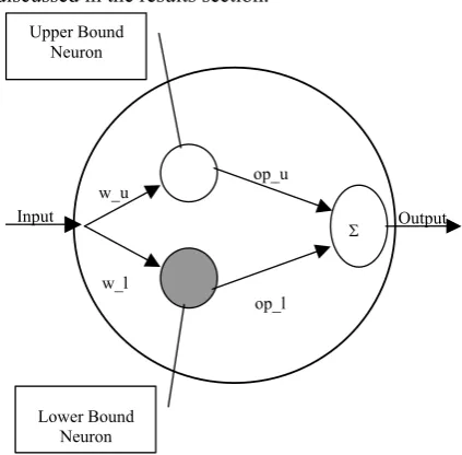
Figure 3 Structure of Rough neuron
IV. ROUGH NEURAL NETWORK
In this section we describe the rough neural network and its constituents. In the first two subsections we discuss the philosophy and structure of the rough neuron. The architectural implementation of the rough neuron into a Kohonen neural system is discussed in the subsequent subsection.
A. Rough Neuron: Philosophy
The rough set primarily deals with the inconsistent part of the data, which is present in any kind of practical system. Using this, one could extract the hidden patterns and explore the data including this inconsistency. Incorporating this into the neural network would help in implementing this over larger applications.
The basic rough neuron proposed by Lingras [1] considers the rough neuron to be a pair of neurons, one dealing only with the reducts extracted using rough sets and the other dealing with the entire set of data, and is implemented over the neural network in supervised mode. In this paper we try to implement the same neuron in the unsupervised mode. The lower neuron [1] deals with the significant (or more contributing) part of the data and the upper neuron deals with the entire data. The architecture of the neuron, which is discussed later, is so designed that the contribution of the significant part is more than the insignificant part. Hence, this leads to faster convergence and better classification of the outputs.
B. Structure of Rough Neuron.
As shown in figure 3 the rough neuron consists of two neurons. The input for both the lower bound neuron and the upper bound neuron can be obtained using two methods: i) Summation of the Squared Euclidean Distance method ii) Dot product of the input vector and the weight vector
method.
Here we are using the first method, i.e., summation of the squared Euclidean distance. So, the input of a neuron is given by (5).
2
(
Input
)
=
∑
(
X
−
weight
)
(5) Here ‘X’ is the input values given to the network and the‘weights’ are randomly initiated at the beginning. The inputs given to the neuron are then passed over a transfer function which will help in normalizing the input [3]. The most commonly used transfer function is ‘sigmoid’ function given by:
1
xF
e
β γα
+
=
+
(6)Where α, β, γ should be optimally fixed in order to generalize the neural network performance. The output of the lower and upper bound neuron is given by the following equations [1]:
(
)
min( (
), (
upper))
lower lower
output
=
F input
F input
(7)(
)
uppermax( (
), (
upper))
lower
output
=
F input
F input
(8) With reference to the figure 3, the combined output of the rough neuron is given by [3]:(
)
(
)
upperlower
output
=
output
+
output
(9) V. NETWORK ARCHITECTUREHere we have implemented the unsupervised Kohonen learning based neural network using the rough neurons. The network contains two layers: input layer and output layer. The input layer acts like a buffer and propagates the inputs from outside the network to the output layer. It is in the output layer that we incorporate the rough neurons. With the given input, the output for each neuron in the output layer is obtained and the one with the least value is adjudged as the winner. The weights of the winning neuron along with its neighbors are updated according to (10).
( )* ( )*(
)
new old old
W
=
W
+
α
t
h t
X
−
W
(10)Where α(t) is the learning constant which varies with time and h(t) is the neighborhood function [3].The learning rate is an important parameter in the learning process. It always lies between 0 to 1. In a rough neural network the training goes in two tiers, i.e., two parallel processes run through the network during parameter approximation, one through the lower neuron and the other through the upper neuron [2]. The learning rates of individual neurons are different and are generally time varying and decreases with the number of iterations. The learning rate of the lower neuron is expected to be more than the upper neuron as it is having significant information, which helps in discerning the patterns
VI. RESULTS
The above-discussed rough set based approaches are implemented at different levels for improving the performance of pattern classifier based on pure unsupervised neural network. Hence the results are to be benchmarked with a pure neural network working with optimal value of learning constant α(t). Thus the classification was first carried out by a pure neural network with set values of iterations as 500, 1000 and 1500 and the learning constant was varied in steps of 0.1 from 0.1 to 0.7 as shown in figure 4. Hence the pure neural network with α(t)=0.4 and 1000 iterations was chosen for benchmarking.
Σ
Input Output
w_u
w_l
op_l op_u Upper Bound
Neuron
Figure 4 Classification efficiency for different α(t) for pure neural network
Figure 5 Classification efficiency for different methods for reducts for pure neural network.
The above rough neural network is implemented over a pattern recognition system developed to classify different alphabets of 18 different fonts. The discretized data set is given to a pure neural network with learning rate α= 0.4 and convergence in 1000 iterations is achieved. The earlier described four methods for attribute reductions are used and graph shown in figure 5 is plotted. The chart shows the efficiency achieved for reductions in number of attributes as number of reducts, from 18 to 26 for each type of reducts method discussed in section III. The graph basically depicts impact of setting different thresholds for the above-discussed algorithm and also the impact on the classification efficiency of a pure unsupervised Kohonen neural network. Different threshold values thus result in generation of different numbers of reducts. The total number of attributes to the preprocessor are 31 which are reduced to 18 to 26 for different values of threshold respectively. From the graph above we conclude that the attribute reductions results in the optimum efficiency.
[image:4.595.56.275.297.419.2]The graph in figure 6 shows the relationship between classification efficiency of rough neural network for the above-discussed four reduction methods. The four methods of reductions not only give the four ways of choosing required number of contributions but also further form the basis of splitting the inputs to the lower and upper bound neurons. Hence, it gives an insight to the impact on
Figure 6 Classification efficiency for four reducts methods for rough neural network.
classifier respective to the type of reduction method chosen. The graph provides us the best reduction method for the set conditions i.e. values of α1(t) and α2(t) and number of iterations obtained by the above step.
The rough neuron consists of 2 neurons namely the upper and the lower. In order to find the optimum learning coefficients for both neurons, the following experimentation shown in Table 1 was carried out. First the α1(t), the learning rate for lower bound neuron is set and then the learning rate of upper bound neuron i.e. α2(t) is varied in steps of 0.1 for iterations of 50 and100 and classification efficiency is observed. Next the α1(t) is changed and the above is repeated. The most optimum values i.e. α1(t), α2(t), and number of iterations are declared for the set or combination which gives the maximum classification of the network. The learning rate for the lower neuron is more than that of the upper bound neuron as the inputs going to the lower one are the more significant ones and the upper neuron has just the entire reduced set, obtained by the preprocessing stage. The significant inputs are those, which can help in discerning between two classes the maximum.
Table 1 Various values for α1(t) & α2(t) for rough neuron
α1(t) α2(t) For 50 Iterations For 100 Iterations
0.2 46.28 % 53.36 %
0.3 45.27 % 52.30 %
0.5
0.4 49.47 % 44.87 %
0.2 49.29 % 48.05 %
0.4
0.3 44.69 % 54.24 %
0.1 52.47 % 51.76 %
0.3
0.2 50.53 % 51.94 %
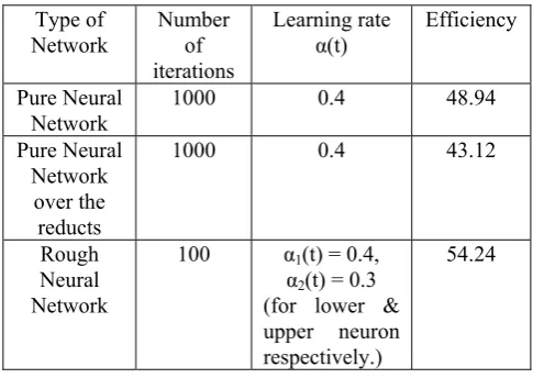
Table 2 Performance of pure vs. rough neural network.
Type of
Network Number of iterations
Learning rate
α(t) Efficiency Pure Neural
Network
1000 0.4 48.94 Pure Neural
Network over the reducts
1000 0.4 43.12
Rough Neural Network
100 α1(t) = 0.4,
α2(t) = 0.3 (for lower & upper neuron
[image:4.595.309.544.486.598.2] [image:4.595.305.548.618.790.2]The results shown in Table 2 clearly demarcate the rough neural network from the conventional neural networks. The classification accuracy, which is calculated as the number of correct recognitions by the total number of samples while testing, shows that the efficiency of the system increases considerably when rough neural network is incorporated. It is further observed that the number of iterations required to get convergence of the system are also less with the rough neural network when compared with the pure neural network, though the time required per iteration is more for the former over later. But in most practical applications neural computing is carried out over parallel processing and hence the time of convergence of the rough neural will be less.
REFERENCES
[1] P. Lingras, “Rough Neural Networks”, In Proc. of the 6th Intl. Conf. on Information Processing and Management of Uncertainty, Universidad da Granada, Granada, 1996, pp. 1445 – 1450.
[2] Jiang-Hong Man: An improved fuzzy discretization way for decision tables with continuos attributes, Proceedings of the Sixth International Conference on Machine Learning and Cybernetics, Hong Kong, 19-22 August 2007.
[3] Sandeep Chandanal, Rene V. Mayorga, “ The New Rough Neuron”, International Conference on Neural Networks and Brain, 2005. ICNN&B '05.
[4] Yassar Hassan, Eiichiro Tazaki, Sina Egawa, Kazuho Suyama,” Rough Neural Classifer System”, IEEE International Conference on Systems, Man and Cybernetics, 2002.
[5] Hongsheng Su, Qunzhan Li: Fuzzy Neural Classifier for Fault Diagnosis of Transformer Based on Rough Sets Theory: IEEE, CS, 2223 to 2227