Applying Peak-Shaving to Household Devices
using an Event-Driven Algorithm
T.G.J. Bolding
University of Twente P.O. Box 217, 7500AE Enschede
The Netherlands
[email protected]
ABSTRACT
Having peaks in the power usage of households requires the electricity infrastructure to have capacity that can be superfluous at most times. Requiring this extra capacity causes higher electricity generation costs, amongst others. This paper proposes an approach using an event-driven al-gorithm that is designed to shave peaks of the total power usage of a household. The approach is able to operate with smart plugs that can be attached to almost any device, no matter how old, hereby making the approach highly flex-ible. The performance of the approach is demonstrated using experiments comprising both real and simulated de-vices. The results of the experiments indicate that the ap-proach has high potential for lowering peaks in the power usage of households.
Keywords
peak-shaving, demand side management, device constraints, intelligent control, slack
1.
INTRODUCTION
The introduction of renewable energy sources (RES) such as wind turbines and photovoltaic (PV) panels, combined with the increasing market share of electric vehicles (EVs) and heat pumps, pose major threats to our current en-ergy infrastructure. In an electricity system, supply and demand need to be balanced to have a working system. When there is too little energy provided, devices cannot work; when there is too much electricity produced, it has no place to go. With non-renewable energy sources we are able to control the supply side of the system. When a lot of electricity is demanded at one moment, we could e.g. raise the heat in our fossil-fuel power station by injecting more fuel. With the introduction of RES this changes, since for example PV panels and wind production are un-controllable energy sources.
To regain control over the balance in the system we use Demand Side Management (DSM). With DSM, the re-sponsibility of keeping the system in balance shifts from the supply side to the demand side. To fulfil this respon-sibility, decisions need to be made on whether to increase or decrease power usage at any given moment.
Permission to make digital or hard copies of all or part of this work for personal or classroom use is granted without fee provided that copies are not made or distributed for profit or commercial advantage and that copies bear this notice and the full citation on the first page. To copy oth-erwise, or republish, to post on servers or to redistribute to lists, requires prior specific permission and/or a fee.
30thTwente Student Conference on ITFebr. 1st, 2019, Enschede, The Netherlands.
Copyright2018, University of Twente, Faculty of Electrical Engineer-ing, Mathematics and Computer Science.
Another use case of DSM is peak-shaving. Peaks occur when a single or multiple devices draw a significantly higher amount of power at one moment, compared to their com-bined nominal power usage. These devices could be lo-cated across a neighbourhood or in a single house. The electricity grid needs production and transport capacity to deal with such peaks, whereas this capacity might barely be used in nominal use. Requiring this capacity means, amongst others, higher transmission and generation costs. Therefore, it is beneficial to have as few, and as little in size, peaks as possible. Peak-shaving tries to minimise peaks by making the overall power usage as constant as possible. This can, for example, be achieved by letting an EV spread its power consumption by charging at a lower power, or letting devices be planned to draw at a higher power sequentially instead of in parallel, hereby preventing simultaneous high usage.
Even though bigger gains can be obtained by applying peak-shaving to e.g. EVs, see for example [4], it is inter-esting to investigate what applying peak-shaving to typical white good devices can yield because these white good de-vices are already in most households. For example, [11] states that refrigerators have an estimated penetration rate of 106% in Europe. Another benefit of trying to con-trol refrigerators is that they can easily be concon-trolled with a smart plug, that needs to do nothing different than being able to measure the power usage and enable and disable the power supply to the refrigerator. These smart plugs can also be used with older refrigerators, that do not have any DSM capabilities of their own, and are therefore easy to use also in households that are not willing to invest in a smart refrigerator.
In this paper, an algorithm is proposed that can apply peak-shaving to household devices by controlling devices with a smart plug, using the total power usage of the household as its main input. Then, the algorithm is demon-strated using real-life experiments. The results of these experiments are analysed and discussed, and afterwards an overview is given on how the proposed algorithm com-pares to related work.
2.
APPROACH
The approach uses a metric calledslack, which expresses the flexibility that a device has left (further explained in section 2.2), to calculate what devices should be turned off. This metric is chosen since it should keep flexibility high while conforming to required objectives. For example, in a hypothetical case of two refrigerators the approach using slack should not get into a situation where only flexibil-ity of one of the refrigerators is used, making it reliant on the second refrigerator only. If in this situation this sec-ond refrigerator would lose its flexibility (for example due to a minimum on/off time requirement), no flexibility to remedy peaks would be left at all.
In this section first the different device classes are explored, then the term slack is explained, and then the proposed algorithm is given. The term system is used to refer to the set of devices controlled by the algorithm.
2.1
Device classes
All devices connected to the algorithm are divided into three classes: Uncontrollables,Time shiftablesand Switch-ables. This division of devices is required to know what can be achieved in terms of control for every device.
2.1.1
Uncontrollables
The class of Uncontrollables consists of all devices that can not be controlled in any manner (for example because of user availability requirements). These devices solely contribute to the total power usage, and are not used any-where else in the algorithm.
Examples: microwave, coffee machine
2.1.2
Time shiftables
Devices in theTime shiftables class are devices of which the power usage profile can not be changed or interrupted, but are shiftable in time, i.e. the starting time can be controlled. At the moment the algorithm does not control devices in theTime shiftables class, but only reads their power usages.
Examples: dishwasher, washing machine
2.1.3
Switchables
Devices in theSwitchablesclass have the most control ca-pability of all considered devices. The power supply to these devices can be interrupted at any moment (respect-ing minimum run-time requirements). Devices in this class often also have a objective to fulfil. For example: a refrig-erator has to keep its internal temperature between e.g. 2 and 7 degrees C.
Examples: refrigerator, air conditioning unit
2.2
Slack
Barker et al. define slack in [1] as ”a measure of how long each background load is able to remain off without affecting its objective”. This slack is expressed in minutes, and gives an abstract number that can be implemented per type of device. For example: when a refrigerator’s internal temperature increases with 0.5°C per minute, its current temperature is 2°C, and its maximum temperature is set at 7°C, it has (7−2)/0.5 = 10 minutes of slack remaining.
2.3
Algorithm
The proposed algorithm is purely event-driven. When a device’s slack or power usage changes, an event is triggered that causes a corresponding method to be called. For the overall system a power usage threshold T is configured. ThisT needs to be set such that on a power usage lower thanT no peak-shaving needs to be applied.
When a device’s slack changes (for example because of an internal temperature change, in the case of a refrigerator), it is calculated whether the current slack still complies with the device’s objective, if not, the supply of power to the device is enabled. In the refrigerator example this en-sures the internal temperature stays within defined limits.
When a device’s power usage changes, the total power usagePsumof the entire system is measured. IfPsum> T,
the differenceδ=Psum−Tis calculated. Then the devices
are sorted in descending order of available slack, giving the sorted list (d1, ..., dn), with n being the number of
devices in the system. Given thatPdi is the power usage
of devicedi, devices (d1, ..., dk), with 1≤k≤n, are chosen
such thatPk
i=1Pdi ≥ δ and
Pk−1
i=1 Pdi < δ if k >1. In
words: (d1, ..., dk) is the set of devices with the most slack
available out of all the devices that are required to be switched off to bring the total power usage below threshold
T.
3.
EXPERIMENTS
To test the proposed algorithm, real-life experiments were conducted.
3.1
Setup
To test the algorithm several real devices and some virtual ones were used. The real devices consisted of two refrig-erators, a microwave, a coffee machine and a dishwasher. Smart plugs of type PlugWise Circle [9] were installed in-between the devices’ plugs and the wall outlet. These Circles measure the power usage of the devices and are able to switch the power supply on and off. In one of the refrigerators a temperature sensor was installed. More on this temperature sensor in section 3.1.1.
The Circles were wirelessly connected to a Raspberry Pi [10] running openHAB2 [8]. The openHAB platform sup-ports Jython [6] scripts to automate the control of the devices and implement the virtual devices. These virtual devices are implementations of a model of a refrigerator, mostly based on one of the real refrigerators of the experi-ment. Section 3.1.2 goes into more details on these virtual refrigerators.
Both the virtual refrigerators and the controlled real-life refrigerator were given a minimum on/off time of two min-utes. This means that when the state of the supply of power is changed (for example from off to on), no change is allowed to occur in the next two minutes. This is to pre-vent damage or lifetime degradation to a (hypothetical) refrigerator caused by rapid switching of the compressor (see e.g. [2]). Although a shorter time than two minutes could probably be sufficient to prevent possible damage, the time is intentionally set long to explicitly show the ef-fects of such a minimum on/off time on the performance of the algorithm.
3.1.1
Temperature sensor
00:00 03:00 06:00 09:00 0
50 100 150
Time
P
o
w
e
r
[W]
4 6 8 10
T
e
m
p
e
ra
tu
r
e
[
°
C
]
[image:3.595.59.279.54.177.2]Power usage Temperature
Figure 1. Sample characteristics of a refrigerator, with temperature sensor placed in the door
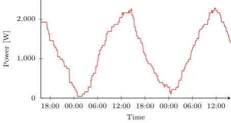
18:00 00:00 06:00 12:00 18:00 00:00 06:00 12:00 0
1,000 2,000
Time
P
o
w
e
r
[W]
Figure 2. Two days of the power usages of forty virtual refrigerators after start-up, summed
to its final place in the door of the refrigerator to ensure connectivity between the transmitting sensor and the re-ceiver. For the virtual refrigerators the speed of change of temperature were derived from the measurements taken from the sensor placed in the door of the refrigerator, but the turn on and turn off temperatures are set further apart, to increase variance between virtual refrigerators. Also note that the actual temperature of the virtual refrigera-tors does not matter for the experiments, as long as each refrigerator has a varying temperature, and thereby slack.
3.1.2
Virtual refrigerators
In the experiments system there is only one real device of which the actual slack can be obtained, namely the re-frigerator which has a temperature sensor installed. Since the effects of the proposed algorithm can hardly be shown with this singleSwitchable device, simulated refrigerators are added.
The virtual refrigerators are modelled with the following characteristics, derived from the characteristics of a real-life refrigerator shown in figure 1:
• The temperature at which the refrigerator would start cooling (if it has power) is set at 7.0°C;
• The temperature at which cooling is stopped is set at 2.0°C;
• The cooling power usage is set at 60W;
• The idling power usage is set at 1.05W;
• The internal temperature increases with 0.005°C each minute when not cooling;
• The internal temperature decreases with 0.01°C each minute when cooling;
• Every minute there is a 1/100 chance of having the refrigerator’s door opened. A door opening increases the refrigerator’s internal temperature with 0.2°C.
When the openHAB system was turned on, each virtual
refrigerator would start in the following state:
• Power supply switched on;
• Internal temperature of either 2.0, 3.0, 4.0, 5.0 or 6.0°C.
The possible internal temperatures were distributed as equally as possible. The behaviour of the virtual refrig-erators after start-up is shown in figure 2.
Although not completely representative compared to real refrigerators, these virtual refrigerators did have charac-teristics that were most important to this research, namely being controllable with an on/off switch, having a signifi-cant power usage at moments (when cooling), and having an easy to read slack characteristic. A linear model for the temperature changes was chosen because of its simplicity.
3.2
Results
The results of the proposed peak-shaving algorithm will be analysed using the functionvpeakgiven by Gerards and
Hurink in [5]. This functionvpeakuses the objective
func-tionM2, which takes a set of power usage measurements
−
→p as input, and is given as
M2(−→p) :=
v u u t1
N
N
X
n=1
p2 n.
The objective function aims to penalise peaks, and does so by squaring the power usage measurements.
vpeak is formulated as
vpeak:=M2(−→p)−M2(
− →
p∗)
where −→p is the vector of power usages measured during baseline measurements, and−→p∗ is the vector of power us-ages measured when the proposed peak-shaving algorithm is applied. The better of a job a peak-shaving algorithm does, the higher the result ofvpeak is expected to be.
3.2.1
Baseline measurements
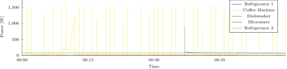
First, we take a look at the power usages of the real de-vices when no control is applied. Figure 3 shows a one hour sample of the power usages of the devices. It is clear to see that there is one specific device (the coffee machine) caus-ing peaks that are approximately seven times the nominal power usage. The lines of the other devices are barely visible.
3.2.2
Five virtual refrigerators
First the algorithm was applied to a system with five vir-tual refrigerators. However, the algorithm was not given control. This phase of the experiments was purely used to investigate the possible actions of the algorithm and whether it was implemented correctly.
What was found is that the power usage of several devices in theUncontrollableclass largely outweighed the flexibil-ity in theSwitchable class (including the virtual devices). During this phase the thresholdT was set at 1.5kW. As can be seen from figure 3 the power usage of only the coffee machine alone was more than 1.5kW at times. Meaning that when this device had such a peak, the algorithm turns off all refrigerators, and when the device did not have such a peak, all refrigerators could be turned on. While this re-sult did show the algorithm was correctly implemented, it also showed this shortcoming in the setup.
3.2.3
Forty virtual refrigerators
[image:3.595.56.283.224.345.2]00:00 00:15 00:30 00:45 0
500 1,000 1,500
Time
P
o
w
e
r
[W]
Refrigerator 1 Coffee Machine
[image:4.595.59.540.57.174.2]Dishwasher Microwave Refrigerator 2
Figure 3. Sample one hour power usage per device
changed from 1.5kW to 2.0kW, to deal with this increase in virtual refrigerators. It was again seen that the algorithm was well implemented, and acted as it was expected to do. However, even though the shortcoming found when using five virtual refrigerators was mostly mended, another shortcoming of the algorithm was found. To demonstrate this shortcoming, figure 4 shows the typical power usages of the forty virtual refrigerators over the period of one hour.
What can be seen is that there are recurring states of having a lot of virtual refrigerators on and having almost none on at all. What was found is that this is an effect of a few factors: the implemented minimum on/off time of two minutes, the fact that the virtual refrigerators them-selves are counted in the total power usage (which is as it is supposed to be), the thresholdT was set too low, and the virtual refrigerators having too little starting variance. Starting at a situation at timetwhere no restrictions on power supplies are in place, the accumulated power usage of the virtual refrigerators is almost 2kW on its own, as can be seen from figure 4. When then a peak happens in one of the real devices, the system would often exceed the thresh-oldT of 2kW. Peaks often occurring were peaks from the coffee machine of about 1.5kW. When one of these peaks occurs the algorithm would switch off the power supply of most devices in theSwitchable class. Since the minimum on/off time then prevents these devices from turning on again in the next two minutes, all slack remaining is in the few Switchable devices that are still on. Now, after these two minutes all devices’ power supplies are switched on again. Again, the power supply status of all of these devices is not allowed to change for two minutes. At the end of the two minutes, the system is in a similar state to the one on timet, causing the cycle to repeat.
16:30 0
500 1,000 1,500 2,000
Time
P
o
w
e
r
[image:4.595.57.285.607.729.2][W]
Figure 4. Typical one hour power usages of
forty virtual refrigerators with algorithm running, summed
However, this does not mean the algorithm did not per-form its job. Taking two five-day samples, one with the algorithm running, and one with the algorithm not run-ning gives the following results:
State M2
Algorithm turned off 1555.09 Algorithm turned on 1264.04
This gives a value ofvpeakof 291.05. Although this value
does not mean much on itself, it could be used to compare the performance of the proposed approach with perfor-mances of different approaches using the same setup.
3.3
Experiments evaluation
In this section the results of the experiments are evalu-ated, and afterwards possible improvements to the setup are listed.
3.3.1
Evaluation of results
The value ofvpeakindicates good performance of the
algo-rithm. Even though cyclic behaviour was found, as shown in figure 4,vpeakindicates that the overall number of, and
size of, peaks has decreased when the algorithm was run-ning, compared to when it was not. It has to be noted that the results are based on five days of measurements. Even though no preference was taken in choosing these days, it could be that external factors contributed to the demonstrated performance of the algorithm. For exam-ple, if in the period where the algorithm was turned off the dishwasher ran, and in the period where the algorithm was turned on it did not, this would possibly influence the value ofvpeaksignificantly.
3.3.2
Possible improvements to the setup
Improvements could be made to the setup to improve the relevance of the results of the experiments. Due to time constraints, these improvements were not implemented dur-ing the course of this research. Even though there most likely are more, three possible improvements stand out, namely that there could be more variation in the virtual refrigerators, that there could be a better spread of devices turning on after a minimum off time, and the experiments should be done over the course of more days.
The variation in virtual refrigerators, and especially their starting values, could be increased so that there is more variance in the amount of slack per refrigerator. Now, the virtual refrigerators show very similar behaviour, as can be clearly seen from figure 2. This can be explained by the fact that there are only five states a virtual refrigerator can have at start-up, namely
• Internal temperature of either 2.0, 3.0, 4.0, 5.0 or 6.0°C.
Following from this is that the only variation between vir-tual refrigerators with the same starting internal tempera-ture is developed over time by the random chance of door openings and different number of times the refrigerator’s power supply is switched of by the algorithm. By adding variance to the starting state, e.g. by having some refriger-ators’ power supply switched off, this synchronisation can be remedied.
Spreading out the turn on moments of the virtual re-frigerators might remedy situations as described in sec-tion 3.2.3, where a cyclic behaviour of the power supply statuses of the virtual refrigerators is observed. Future research would have to show whether spreading out the power supply switch on moments would actually remedy this problem. Gerards and Hurink in [3] propose a method designed to enable DSM algorithms to incorporate mini-mum run-time constrained devices that might be of use when improving the algorithm proposed in this paper.
As noted in section 3.3.1 the time span of the experiments might have been to short to conclusively show the per-formance of the approach. Future research would have to re-run the experiment with a larger time span to prove the performance of the proposed algorithm more conclusively.
4.
COMPARISON TO RELATED WORK
4.1
SmartCap
Barker et al. in [1] propose an approach called SmartCap that is very similar to the one proposed in this paper. They also propose an online scheduler that chooses which devices to turn off based on the devices’ slack, and they also only deal with on/off switching. There is however one major difference between their approach and the one proposed in this paper; where their approach calculates what devices to give power once every minute, the one in this paper reevaluates the division of power on each power usage change.
A possible drawback of their approach lies in a situation where the power usage division is calculated at time t, and then a peak occurs a second later. Their approach would only respond to this peak almost a full minute later, whereas the approach proposed in this paper would theo-retically respond to the peak immediately.
This event-based nature of the approach proposed in this paper does have a possible drawback compared to the one presented by Barker et al. however. In a situation where multiple power usage changes occur within a very short time span, the controlling system might not be able to cal-culate its actions before a new change occurs. This could potentially cause a situation where the difference in time between a change occurring and its consequences being applied would continue to grow, since the system cannot find a time to process the entire ”backlog” of changes. A possible solution to this problem would be to discard trig-gers while processing a previous one, but further research needs to be done to find the implications of this change. Note that no manifestation of this possible drawback was noticed during the experiments described in this paper.
4.2
Robust EV peak-shaving
Gerards and Hurink in [4] propose an online planning al-gorithm initially designed to control the charging of EVs in a neighbourhood. The algorithm is designed such that it has a low communication overhead and uses few inputs. Even though this algorithm can adjust its predictions at
the start of an interval, it still has the same characteris-tic as SmartCap, where a sudden peak is not dealt with until the start of a new interval. The algorithm from [4] is more suited to reducing large, long-lasting peak loads, in contrast to the approach presented in this paper that is designed for sudden peaks, and probably is more suited to deal with short peaks. Research would have to show how well the peak-shaving algorithm from [4] performs in a situation with sudden and short peaks.
5.
CONCLUSIONS AND DISCUSSION
In this paper an approach was presented to apply peak-shaving to household devices, using only simple smart plugs to control and measure the devices. Using an ex-periment that included several real devices, as well as simulated ones, it was shown that the proposed approach seems to perform well. It has to be noted that these re-sults were based on measurements taken from experiments that spanned five days. External factors could have played a significant role in the perceived performance of the ap-proach. Still, it is expected that the approach has signif-icant potential based on the value of vpeak. Also, even
though the approach is only applied to controlling refrig-erators in this paper, it would need no adaptations to also control freezers, which have a much larger potential for use as a buffer device according to [7]. Also other devices such as air conditioning units could be incorporated in a system using the proposed approach without further adaptations to the approach itself.
6.
FUTURE WORK
Future work could be performed to improve the approach and the knowledge about its characteristics. In this section several topics for future work are listed.
6.1
Incorporation of control of devices in the
Time shiftables class
In its current form, the approach uses power usage mea-surements from devices in theTime shiftables class, but does not control them, even though high flexibility can be offered by some of these devices (see for example [7]). It therefore is interesting to research how these devices can be incorporated in the proposed approach. A possible ap-proach would be to implement theTime shiftablesdevices’ slack function as reaching 0 when
6.2
EV (dis)charging
The charging and possible discharging of an EV can offer large amounts of flexibility to a system (see for example [7]). Again, incorporating EV (dis)charging into the ap-proach is therefore highly interesting. It could be a pos-sibility that the (dis)charging of EVs can be incorporated by regarding the charger as a device in the Switchables
class and introducing a device-specific slack function. For example, this function can be defined such that slack is 0 when the charger needs all available time until planned departure time to complete charging. Barker et al. use a similar method in [1] to incorporate EV charging into their scheduler. Future research would have to show whether it indeed is a possibility to incorporate EV charging into this paper’s approach, and what the resulting performance would be.
6.3
Setting the threshold
TIn the experiments in this paper, it was attempted to set
setting. Therefore, it needs to be investigated what a good method for finding the best value forT is.
6.4
Dealing with possible controller
overload-ing
In section 4.1 a possible problem is presented where the controller would be overloaded with changes in power us-age and/or slack. It needs to be researched whether this problem could actually present itself. It is highly possible that with the processing speed of current-day computers, such a problem cannot occur. However, when the number of devices connected to the controller is increased, also the load on the controller is increased. For example, no con-troller would be able to handle an infinitely high frequency of power usage/slack changes with the approach presented in this paper. This means that for any controller there is a maximum frequency of changes it can handle before the problem mentioned in section 4.1 would occur. It could be interesting to research if the possibility of reaching this maximum would limit the possible applications of the pro-posed approach.
7.
ACKNOWLEDGMENTS
The author would like to thank Marco Gerards and Gerwin Hoogsteen for their supervision and valuable input during the course of this research.
8.
REFERENCES
[1] S. K. Barker, A. K. Mishra, D. E. Irwin, P. J. Shenoy, and J. R. Albrecht. Smartcap: Flattening peak electricity demand in smart homes. In
PerCom, pages 67–75, 2012.
[2] B. Biegel, P. Andersen, T. S. Pedersen, K. M. Nielsen, J. Stoustrup, and L. H. Hansen. Smart grid dispatch strategy for on/off demand-side devices. In
2013 European Control Conference (ECC), pages 2541–2548, July 2013.
[3] M. E. T. Gerards and J. L. Hurink. Planning of on/off devices with minimum run-times. In2016 IEEE PES Innovative Smart Grid Technologies Conference Europe (ISGT-Europe), pages 1–6, Oct 2016.
[4] M. E. T. Gerards and J. L. Hurink. Robust peak-shaving for a neighborhood with electric vehicles.Energies, 9(8), 2016.
[5] M. E. T. Gerards and J. L. Hurink. On the value of device flexibility in smart grid applications. 6 2017. 12th IEEE PES PowerTech Conference : Towards and Beyond Sustainable Energy Systems, PowerTech 2017 ; Conference date: 18-06-2017 Through 22-07-2017.
[6] The jython project.http://www.jython.org/. Accessed 14-January-2019.
[7] B. P. V. Meerssche, G. V. Ham, and G. Deconinck. Analyzing loads for balancing: Potential for the belgian case. In2012 IEEE Power and Energy Society General Meeting, pages 1–8, July 2012. [8] openhab.https://www.openhab.org/. Accessed
2-December-2018. [9] Plugwise circle.https:
//www.plugwise.com/nl_NL/products/circle. Accessed 2-December-2018.
[10] Raspberry pi - teach, learn, and make with raspberry pi.https://www.raspberrypi.org/. Accessed 2-December-2018.
[11] R. Stamminger, G. Broil, C. Pakula, H. Jungbecker, M. Braun, I. R¨udenauer, and C. Wendker. Synergy
APPENDIX
A.
REFRIGERATOR CHARACTERISTICS SAMPLES
A.1
Sample characteristics of a refrigerator, with temperature sensor placed in door
00:00 01:30 03:00 04:30 06:00 07:30 09:00 0
50 100 150
Time
P
o
w
e
r
[W]
4 6 8 10
T
e
m
p
e
ra
tu
r
e
[
°
C
]
Power usage Temperature
A.2
Sample characteristics of a refrigerator, with temperature sensor placed in the middle of
the refrigerator
00:00 01:30 03:00 04:30 06:00 07:30 09:00 0
50 100 150
Time
P
o
w
e
r
[kW
]
4 6 8 10
T
e
m
p
e
ra
tu
r
e
[
°
C
]