On properties of the American put option under several models

(1)

warwick.ac.uk/lib-publications

A Thesis Submitted for the Degree of PhD at the University of Warwick

Permanent WRAP URL:

http://wrap.warwick.ac.uk/95313

Copyright and reuse:

This thesis is made available online and is protected by original copyright.

Please scroll down to view the document itself.

Please refer to the repository record for this item for information to help you to cite it.

Our policy information is available from the repository home page.

(2)

On properties of the American put

option under several models

by

Yufan Zhao

1164727

A thesis submitted in partial fulfilment of the requirement for

the degree of

(3)

Acknowledgements

(4)

Declarations

The work contained in this thesis is original, except as acknowledged, and has not been submitted previously for a degree at any university. To the best of my knowledge and belief, this thesis contains no material previously published or written by another person, except where due reference is made.

(5)

1 Introduction and Preliminaries

The central theme of this thesis is the application of optimal stopping in American option pricing. The purpose of this chapter is to provide a literature review of the techniques used throughout this thesis.

1.1 Optimal stopping problems

The theory of optimal stopping is concerned with the problem of choosing a time to take a particular action, in order to maximise an expected reward or minimise an expect cost. Optimal stopping theory has a long history. In 1947, Wald [75] investigated the problem of sequential testing. Snell [68] formulated a general optimal stopping problem for discrete time stochastic processes and characterised the solution by the means of smallest supermartingale dominating the gain sequence, which came to be known as Snell’s envelope.

However, a general theory of the subject did not exist until the 1960s. In February 1960 copy of Scientific American, the famous Secretary Problem was discussed. The solution of which was suggested and proven by Dynkin [21]. In the 1963 paper, Dynkin also formulated a general optimal stopping problem for Markov processes and characterised the solution as the smallest superharmonic function dominating the gain function.

The 1960s and 70s saw major developments of general optimal stopping theory. [22, 23, 24, 25, 26, 29, 30, 40, 64, 65, 66] is a small sample of the extensive literature from this period. For a survey of optimal stopping problems and general theory of optimal stopping for Markov processes, [67] by Shiryaev is a good reference.

The classical applications of optimal stopping include mathematical statistics, stochastic analysis and financial mathematics. We refer to [57] and references within. The most relevant application of optimal stopping to this thesis is option pricing in the field of financial mathematics. The most famous example is the work on Black-Scholes model by McKean [49].

The purpose of this section is to review some of the standard techniques used in the existing literature for optimal stopping problems. We refer to [57, 67] for a comprehensive review. Some of the results we quote in this section are taken from these references.

We begin by defining optimal stopping problems in a standard set-up. In general, we are interested in optimal stopping problems with respect to strong Markov processes. Let

X = (Xt,Ft : t ≥ 0) be a strong Markov family defined on a measurable space (Ω,F) taking values in a measurable spaces (E,B), together with a family of probability measure

{_Px}_x∈E. These probability measures have the property Px(X0 = x) = 1 and (Xt)t≥0 is

(8)

Intuitively, we can only make a decision about when to stop based on the information we already know. This is why the concepts of stopping time and Markov time are required.

Definition 1.1. We define a Markov time to be a random variableτ such that{τ ≤t} ∈ F_t

for allt≥0. A stopping time is a Markov time τ such that P(τ <∞) = 1. For a given measurable function,g:E →_Rwhich satisfies the condition

Ex(sup t≥0

|e−rtg(Xt)|)<∞ for all x∈E, (1.1) we are interested in finding the value function

V(x) = sup τ∈T_[0_,∞]

Exe−rτg(Xτ). (1.2)

whereT_[0_,_∞]is the set of all stopping times with respect to (Ft)t≥0andrshould be a positive

constant. Here e−rt represents a discount term, which can represent the opportunity cost for stopping later rather than sooner. The case r ≤0 can lead to V being infinite and/or a stopping time does not exist, see Remark 2.2 for an example. This is referred to as an infinite horizon problem. Usually, we will dropT_[0_,∞] from our notation.

The corresponding finite time horizon problem is

V(x, t) = sup

0≤τ≤T−tEt,x

e−rτg(Xt+τ), (1.3) This can be seen as replacing the Xt in equation (1.1) by the process Zt = (t, Xt) for

t ≥ 0 with the state space R+ ×E. By (1.3), we arrived at the terminal condition

V(x, T) =g(x) by settingt=T.

We refer toV as thevalue function andg as the gain function. The value function can be written in this simple form due to the Markov property of the process X. All of the processes we deal with in this thesis are Markov processes, so it is sufficient for our purposes to address the theory of optimal stopping in this form only. In addition to the value function, we are also interested in the stopping rule we need to apply to stop optimally, so we give the following definition:

Definition 1.2. We say that τ∗ is an optimal stopping time if

V(x) =Ex(e−rτ

∗

g(Xτ∗)). (1.4)

(9)

into two sets:

C={x∈E :V(x)> g(x)}, (1.5)

D={x∈E :V(x) =g(x)}. (1.6) We refer to C as the continuation region andD as the stopping region. IfV is lower semi-continuous and gis upper semi-continuous, then C is open and Dis closed. Provided that the process X satisfies (1.1), then we have the following sufficiency theorem for optimal stopping.

Theorem 1.3 (Theorem 2.7 in [57]). Assume that the gain function g:E →_R satisfying the condition

Ex(sup t≥0

e−rt|g(Xt)|)<∞ for all x∈E.

Assume that there exists a smallest function Vˆ which dominates the gain function g on E such thate−rtVˆ(Xt) is a supermartingale with respect to Px for x∈E.

Let us in addition assume that Vˆ is lower semi-continuous (lsc) and g is upper semi-continuous (usc). Set Dˆ ={x∈ E : ˆV(x) =g(x)} and let τ_Dˆ = inf{t≥0 : Xt ∈Dˆ}. We

then have:

(1) if Px(τ_Dˆ <∞) = 1 for x∈E, then Vˆ =V and τ_Dˆ is optimal in (1.2),

(2) if Px(τ_Dˆ < ∞) < 1 for some x ∈ E, then there is no optimal stopping time (with

probability 1).

In the case when V is lsc, this is equivalent to the statement V(x) is an r-excessive function. It turns out this r-excessive function characterisation is not only a sufficient condition the value function needs to satisfy, but also a necessary condition. Let us define

τD by

τD = inf{t≥0 :Xt∈D},

which is a Markov time with respect to (Ft)t≥0. We have the following necessary condition

for optimal stopping.

Theorem 1.4 (Theorem 2.4 in [57]). Let us assume that there exists a stopping time τ∗

such that (1.4) holds for all x∈E, then

(1) e−rtV(Xt)is the smallest right-continuous supermartingale underPx such thatV(x)≥

g(x) for all x∈E.

In addition, if V is lsc and g is usc, then we have:

(10)

(3) The stopped process {e−r(t∧τD)_V₍_X

t∧τD) : t ≥ 0} is a right-continuous martingale

underPx for every x∈E.

Remark 1.5. It is useful to make the following observations.

(i) Theorem 1.3 and Theorem 1.4 also hold for finite horizon problem where we would replaceV(Xt) byV(Xt, t).

(ii) In finite time horizon problems, due to the terminal conditionV(T, x) = g(x), τD is an optimal stopping time withτD ≤T.

In infinite horizon problems, there may not exist an optimal stopping timeτ∗ at which the value functionV is attained. However, by the definition ofV, for all >0, there exists a stopping timeτ∗ such that

V(x)−≤Ex(e−rτ∗_g₍_X τ∗

)) (1.7)

A stopping time satisfying equation (1.7) is known as an-optimal stopping time. (iii) When an optimal stopping time does not exists, sometimes we can find Markov time

τ∗ such that (1.4) holds. If τD is a Markov time instead of a stopping time and P( lim

t→∞e

−rt_g₍_X_t) _→ _{0) = 1, then (1.4) still holds with a Markov time} _τ∗ ₌ _τ

D with the convention e−rτ∗g(Xτ∗) = 0 when τ∗ = ∞. This is the case in some of the

problems we will discuss in Chapter 2-4.

(iv) When we cannot solve the optimal stopping problem explicitly, we are still interested in the nature of the continuation region and its boundary, as this allows us to characterise the optimal stopping rule. Literature in this area include [37, 20].

An implication of Theorem 1.3 and Theorem 1.4 is that solving an optimal stopping problem (1.4) is equivalent to finding the smallest r-excessive function ˆV such that ˆV ≥g. In this case,V(x) = ˆV(x) for x∈E and ˆτD defined in Theorem 1.3 is an optimal stopping time ifPx(τ_Dˆ <∞) = 1 for allx∈E.

Generally, it can be quite difficult to search for and identify the smallest r-excessive function directly hence Theorem 1.3 is often not a practical method for solving an optimal stopping problem. An alternative approach is known as the guess and verify approach.

1.1.1 Guess and Verify

Instead of trying to identify the smallestr-excessive function, we can try to identify an opti-mal stopping rule. The stopping time associated with this ruleτ would produce a function

ˆ

(11)

The result below is often referred to as the guess and verify lemma. See [1, 11, 53, 71] for examples of its application.

Lemma 1.6. Consider the optimal stopping problem given by (1.2) with g ≥0. Let τ be a stopping time and Vˆ :E → _R be a function such that the following three conditions are satisfied

(i) Vˆ(x) =Exe−rτg(Xτ),

(ii) Vˆ(x)≥g(x) for all x∈E,

(iii) the process {e−rtVˆ(Xt) : t ≥ 0} is a right-continuous supermartingale under Px for

allx∈E,

thenV = ˆV and τ is an optimal stopping time.

One advantage of this approach is that some properties of the value function does not need to be proved. For example, we often expect the value function to solve a free-boundary problem with a smooth pasting condition. By imposing a smooth pasting conditioning and verifying that the solution of the free-boundary is the value function, we do not need to prove the pasting condition. This lemma is used extensively in Chapter 3.

On the other hand, it is sometimes difficult to guess the value function. Even if we guessed the stopping rule correctly (or proved that it must be of a certain form), the verification procedure can be difficult. This problem is highlighted in Chapter 2 for the Regime Switching model. This method, in general, does not work in finite time horizon because of the stopping region depends on time. It is generally difficult to compute the expected value of the gain function at bounded stopping times.

1.1.2 Free-boundary approach

One approach in solving optimal stopping problems is by solving a free boundary problem. Let us assume thatX solves an SDE

dXt=b(Xt)dt+σ(Xt)Bt (1.8) and c∈_R. If we assume thatV is sufficiently regular, then by Itˆo’s formula, we have that

Exe−rtV(Xt) =V(x) +Ex

Z t

0

(L−r)V(Xu)1{Xs6=c}du +1

2

Z t

0

(V0(Xs+)−V0(Xs−))1{Xs=c}dl c

s(X) +Mt

, (1.9)

where L is the infinitesimal generator ofX, lc

(12)

If we know the stopping regionDand the continuation regionC given by (1.5) and (1.6) are characterised by some value of c, for example, if

C ={x:x > c},

then it is nature to guess thatV is the unique solution the problem

(L−r)V(x)≤0 forx6=c (1.10)

(L−r)V(x) = 0 forx∈C (1.11)

V(x) =g(x) forx∈D (1.12)

V(x)≥g(x) forx∈R (1.13)

V0(c) =g0(c) (1.14)

and Mt is a martingale. It can often be verified by Lemma 1.6 that the unique solution to (1.10) to (1.14) is the value function. A modified version of this Ansatz exists when

X is multidmensional, has jumps or the problem is in finite horizon. This is known as a free-boundary problem because the boundaryc is unknown.

Some optimal stopping problems can be solved explicitly by finding the unique solution to their related free-boundary problems. A classical example of this is the McKean problem [49]. In higher dimension, it may be possible to derive a Volterra type integral equation from the free-boundary problem. One needs to verify that the unique solution of integral equation is the value function. See [57, Theorem 25.3] for how this is done for the finite horizon Black-Scholes American put problem. The condition V0(c) =g0(c) is often known as a ‘smooth pasting’ condition. This condition first appeared in papers by Mikalevich [52] and [51]. Other works on smooth pasting include [14, 10, 49, 36].

The potential difficulty in using the free-boundary approach is two-fold. Firstly, it is necessary to show the uniqueness of the solution to the free-boundary problem. For the finite horizon American put problem under Black-Scholes model, the uniqueness of solution to the integral equation was not proved until 2005 in [56].

Secondly, it is often difficult to verify that the (unique) solution to the free-boundary problem is indeed the solution to the optimal stopping problem. This problem is discussed extensively for the Regime-Switching model in Section 2.1.3. This is why the notion of viscosity solution introduced in the next section comes in handy.

1.2 Viscosity Solutions

(13)

of viscosity solution can be used for studying optimal stopping problems. Consider the variational inequality

min(−(L−r)V(x), V(x)−g(x)) = 0. (1.15) This is an alternative way to write the free boundary problem given by equations (1.10) to (1.14). One can check that if a function satisfies the free boundary problem in the classical sense, then it also satisfies (1.15), except at the stopping boundary c. Viscosity solutions provide us with a weaker notion of solution which is consistent with the classical definition and allows the value function of optimal stopping problem (1.2) to be a solution of this equation (1.15).

The theory of viscosity solutions was initially developed only for first order PDEs, but this was soon extended to integral partial differential equations (abbreviated as IPDEs or PIDEs). These are partial differential equation operators with non-local parts. One of the first papers on viscosity solutions for PIDEs was [70] by Soner, which extended the viscosity solution framework to piecewise-deterministic jump processes with bounded coefficients. This work was then extended by Sayah in [63].

It was initially unknown whether second order elliptic equations admit unique viscosity solutions in general. The breakthrough came in 1988, when Jensen proved a comparison principle in [38]. For a comprehensive account of viscosity solution for degenerate ellipitic second order partial differential equations, we refer to the User’s guide [19]. For papers related to second order degenerate elliptic PIDE, we refer to [4, 5] and references within. The first applications of viscosity solution in optimal stopping include [55] and [59].

The theory of viscosity solution applies to PDEs of the form

F(x, u, Du, D2u) = 0, (1.16) whereF :RN×R×RN×S(N)→Ris continuous andS(N) is the set of symmetricN×N matrices. Du andD2u denote the gradient and the second derivative matrix of u.

Furthermore, F is required to satisfy the fundamental assumption,

F(x, r, p, X)≤F(x, s, p, Y) whenever r≤sand Y ≤X. (1.17) where r, s ∈ _R, x, p ∈ _RN_{, X, Y} _∈ _S₍_N_{). If (1.17) is satisfied by} _F_{, then} _F _{is said to be} proper.

(14)

Definition 1.7. Let F satisfy (1.17) and O ⊂RN. A continuous viscosity subsolution of

F = 0on O is a continuous function u such that for every C2 functionφ such that xˆ is a local maximum of u−φ, then

F(ˆx, u(ˆx), Dφ(ˆx), D2φ(x))≤0.

Similarly, a continuous viscosity supersolution of F = 0 is a continuous function u such that for every C2 function φsuch that xˆ is a local minimum of u−φ, then

F(ˆx, u(ˆx), Dφ(ˆx), D2φ(x))≥0. u is a solution if it is both a subsolution and a supersolution

An equivalent formulation of viscosity solution property is in terms of semijets. The superjets of u atxis given by

J_O2,+u(x) =

(p, X)∈_RN×S(N) :u(ˆx)≤u(x)+p(x−x0)+1 2(x

0₋_x₎T_X₍_x0₋_x₎₊_o _|_x₋_x0_|2

.

the subjets of u atxis defined by

J_O2,−u(x) =−J_O2,+(−u(x)).

It is possible to show that for all (p, X)∈J_O2,+u(x), there exists aC2 functionφsuch that

u−φhas a local maximum at x with Dφ(x) = p and D2φ(x) = X. Hence, an equivalent definition of viscosity solution is in term of these semijets.

Definition 1.8. Let F satisfy (1.17) and O ⊂_RN_{. A continuous viscosity subsolution of}

F = 0 on O is a continuous function u such that

F(x, u(x), p, X)≤0 for allx∈ O and (p, X)∈J_O2,+u(x).

Similarly, a continuous viscosity subsolution of F = 0 is a continuous function u such that

F(x, u(x), p, X)≥0 for allx∈ O and (p, X)∈J_O2,−u(x).

We have now defined the notion of the viscosity solution. It is possible to show that the value function is the viscosity solution to a variational inequality.

Theorem 1.9(Theorem 5.2.1 of [60]). Recall the definition ofV given by (1.2), where the gain function g is now assumed to be Lipschitz. Assuming that r is sufficiently large, then

(15)

Similar results exist if the optimal stopping problem is a finite time horizon one or the underlying process has jumps. As a consequence, the definitions of the subsolution and supersolution need to be adjusted accordingly. We will introduce case specific definitions of supersolution and subsolution in Chapter 2 and 4. Since the notion of viscosity solution is consistent with the classical definition of solution of a PDE, we can apply regularisation arguments to prove properties of the value function without solving for the value function. The regularisation arguments in Chapter 4 will need uniqueness theorem of the following type.

Theorem 1.10(Theorem 3.3 of [19]). Let Ωbe a bounded open set inRN, F ∈C(Ω×R× RN, S(N)) be proper and satisfy the conditions

(i) There exists γ >0 such that

γ(r−s)≤F(x, r, p, X)−F(x, s, p, X) for r ≥s

(ii) There is a function ω: [0,∞]→[0,∞]that satisfies ω(0+) = 0 such that

 



F(y, r, α(x−y), Y)−F(x, r, α(x−y), X)≤ω(α|x−y|2₊_|_x₋_y_|₎

whenever x, y∈Ω, r∈_R, X, Y ∈S(N), and X,Y satisfy the equation

−3α I 0

0 I

!

≤ X 0

0 −Y

!

≤3α I −I

−I I

!

Let u be a continuous subsolution on Ω and v be a continuous supersolution of F = 0 in Ω

and u≤v on ∂Ω, then u≤v in Ω¯.

1.3 Outline of this thesis

The content of the rest of this thesis is outlined below.

Chapter 2 This chapter is dedicated to the Regime Switching model. In the first part of chapter, we study optimal stopping problems under the Regime-Switching model using the notion of viscosity solution. We correct some of the discrepancies in the existing literatures about the perpetual American put problem. In the second part of this chapter, we strengthen an existing result on the monotonicity property of option price in volatility and discuss its implication for numerical schemes.

(16)

model can be found explicitly. For certain choice of parameters, it has an interesting feature that the stopping region is disconnected. We end this chapter with a numerical analysis section with discussions.

(17)

2 On Optimal Stopping under Regime-Switching and

Re-lated Models

2.1 Introduction

2.1.1 Literature review and chapter summary

As noted by many authors, the Black-Scholes model despite being very successful, does not have many desired properties of a market model. One relatively simple attempt to add extra randomness to the model is to let the volatility and rate of return be functions of a finite state Markov chain.

Under the Regime-Switching model, we take a probability space (Ω,F,P) which supports two independent Markov processes (Wt)t≥0 and (It)t≥0, whereW is a Brownian motion and

I is annstate continuous time Markov chain with state space {1, . . . , n}. LetStbe driven by the stochastic differential equation

dSt=σ(It)StdWt+µ(It)Stdt, (2.1) whereσ :{1, . . . , n} →(0,∞) and µ:{1, . . . , n} →(−∞,∞) are known functions. TheSt governed by (2.1) is referred to as a process with ‘Regime-Switching’ or a ‘Markov modulated geometric Brownian motion’ by the existing literature. Intuitively, the Markov chain can be regarded as modelling the business cycle or some economic indicator. It is straightforward to see, when the functionsµand σ are chosen to be constant functions, or n= 1, then this model reduces to the Black-Scholes model.

This model has been subject to intense studies. From an option pricing perspective, see Guo [32] for closed-form solutions for pricing European and perpetual lookback option; Yao, Zhang and Zhou [76] for numerical results for European stock options. Two papers on pricing perpetual American puts are particularly relevant to this chapter: one by Guo and Zhang, [33], treating the case of two-states Markov chains and another by Jobert and Rogers, [39], treating the general case with finitely many states. In addition, the work by Buffington and Elliot, [12], studied the two-state finite horizon American put problem.

This chapter has two parts. First, we introduce the probabilistic set-up for the Regime-Switching model and present the existing results in [33] and [39]. We are unable to follow some of the arguments in [33, 39]. It appears that the proofs of the main results in these papers are incomplete. We examine these in detail and demonstrate how the problems in [33, 39] can be addressed using viscosity solutions.

(18)

options. We demonstrate that our results on American put options are consistent with existing results on the Black-Scholes model by McKean [49] as well as numerical results found in [15] and [42]. We end this chapter with a discussion of open problems and some conjectures based on our results.

2.1.2 Probabilistic set-up for the Regime-Switching model

We recall the probabilistic set-up given in the paragraph preceding equation (2.1). The Regime-Switching processSt is governed by

dSt=µ(It)Stdt+σ(It)StdWt,

and adapted to F_t which we take to be the complete augmented filtration generated by

σ((Ws, Is) :s≤t). We denote the generator matrix ofI by Λ and useλij denote its entries. This means, for i6=j,λij is the jump rate from state ito state j. For i=j, λii is the total rate leaving state imultiplied by −1. In addition, denote the total rate leaving i by

λi, i.e.

λi

def

=−λii.

We construct a family of these processes with initial values S0>0 andI0 ∈ {1, . . . , n}.

We use Ss,i to denote the process S with S0 = s and I0 = i. Similarly, we use Ii to

denote the process I with I0 = i. (The distribution of future value of I does not depend

on current or past values ofS, when conditioned on its current value.) S_ts,i has the explicit representation

S_ts,i=sexp

Z t

0

µ(I_qi)−1

2σ(I i q)2dq+

Z t

0

σ(I_qi)dWq

. (2.2)

It is also useful to defineX_tx,i = logS_ts,i, wherex= logs. Explicitly, we have that

X_tx,i =x+

Z t

0

µ(I_qi)−1

2σ(I i q)2dq+

Z t

0

σ(I_qi)dWq.

The pairs (Ss,i, Ii) and (Xx,i, Ii) are both Markov processes. Let g and h be real functions such that g : (0,∞)× {1, . . . , n} →R and h : (0,∞)× {1, . . . , n} → R. We are interested in the value function associated with the optimal stopping problem

u(s, i) = sup τ E

e−

Rτ

0 r(Iti)dt_g₍_Ss,i τ , Iτi) +

Z τ

0

e−r(Iti)t_h₍_Ss,i t , Iti)dt

fors >0, i∈ {1, . . . , n},

(19)

times with respect toFt. This problem also has the representation

˜

u(x, i) = sup τ E

e−

Rτ

0 r(I

i

t)dt_g_˜₍_Xx,i τ , Iτi) +

Z τ

0

e−r(Iti)t˜_h₍_Xx,i t , Iti)dt

, (2.4)

where ˜g, g,˜h, h,u, u˜ are related by ˜g(x, i) =g(ex, i), ˜h(x, i) =h(ex, i), ˜u(x, i) =u(ex, i). We assume that there is anr <minn_i₌₁r(i) such that

Esup t≥0

e−rtg(S_ts,i, I_ti)<∞ and Esup t≥0

Z t

0

e−ruh(S_us,i, I_ui)du <∞ (2.5) are satisfied, hence u(s, i) is finite. We define the regions Ci and Di for i = 1, . . . , n as follows:

Ci ={s:u(s, i)> g(s, i)}, Di ={s:u(s, i) =g(s, i)}. (2.6) It is straightforward to see that the Ci’s and the D_i0s partition the state space into contin-uation regions and stopping regions according to the value ofi. Similarly, define

˜

Ci ={x: ˜u(x, i)>g˜(x, i)}, D˜i ={x: ˜u(x, i) = ˜g(x, i)}.

In what follows, we shall use the notation σi = σ(i), µi = µ(i) and ri = r(i) for

i∈ {1, . . . , n}. If f : (0,∞)× {1, . . . n} →_R is a function such that f(·, i)∈ C_b2(0,∞) for everyi, then the infinitesimal generator of the pair (S, I) acting on f is given by

Lf(s, i) = 1 2σ

2

is2∂11f(s, i) +µis∂1f(s, i)−λif(s, i) +

X

j6=i

λijf(s, j).

Similarly, for a function f : (−∞,∞)× {1, . . . , n} →_R such that f(·, i)∈C_b2(−∞,∞) for everyi, the infinitesimal generator of the pair (X, I) acting on f is given by

˜

Lf(x, i) = 1 2σ

2

i∂11f(x, i) + (µi− 1 2σ

2

i)∂1f(x, i)−λif(x, i) +

X

j6=i

λijf(x, j).

(20)

2.1.3 Existing results on the American put problem under the Regime-Switching model

The American put is a case of (2.3) where

g(s, i) = (K−s)+ h(s, i) = 0 fors >0, i={1, . . . , n}.

It is claimed in [39, Prop. 2] that, forµi ≤ri, if thresholds ˜bi < log(K) have been found such that the unique bounded solution ˜f to the coupled system of ODEs

( ˜L−ri) ˜f(x, i) = 0 forx >b˜i, ˜

f(x, i) =K−ex forx≤b˜i,

isC1 inxat (˜bi, i) for everyi, then the ˜bi’s are uniquely determined and ˜u(x, i) = ˜f(x, i). If this result holds, by a simple change of variable, we have thatu(s, i) is the unique bounded function satisfying

(L−ri)f(s, i) = 0 fors > bi, (2.7)

f(s, i) =K−s fors≤bi. (2.8)

such that f(·, i) is C1. Here, bi = exp(˜bi), is the stopping level for S when I is in state i. The result is stated in [33] in term off for the case n= 2, µi ≥0 andr1 =r2>0. In the

two-states case, the solution is semi-explicit.

Attempts were made in [39, 33] to check that the solution to system of coupled ODEs are indeed the value functions. These attempts used ‘guess and verify’ methods. If we want to check thatf =u by Lemma 1.6, we need to show the following conditions hold:

(v1) f(s, i) =E[e−

Rτ

0 r(I

i

q)dq_g₍_Ss,i τ )]

(v2) e−R0tr(Iqi)dq_g₍_Ss,i

t ) is a supermartingale for alls >0,i∈ {1, . . . , n}. (v3) f(s, i)≥(K−s)+.

In [39, Prop. 1], the authors claim that the stopping regions Di must be of the form

Di = (0, bi) assumingµi =ri. However, their argument only requires Sts,ie

−Rt

0r(Iqi)dq _{to be} a supermartingale, which holds ifµi ≤ri.

Remark 2.2. [39, Prop. 1] seems to hold even if ri ≤ 0. We briefly comment on the consequences when the discount term is non-positive. When ri ≤0,µi< 1₂σi2,X

x,i

t → −∞ almost surely. For anyη < K, consider the stopping time τηs,i= inf{t:S_ts,i≤η}, then

u(s, i)≥_Ee−rτηs,i₍_K₋_Ss,i τηs,i

)+=Ee−rτ s,i

(21)

Since η is arbitrary, we have that

u(s, i) =

 



∞ forr <0

K forr= 0.

In these cases, an optimal stopping time (or Markov time) does not exist.

When examined more closely, it looks to us that they assumed that an optimal stopping time exists and applied Doob’s optional sampling theorem to an unbounded martingale with this stopping time. It turns out [39, Prop. 1] can be proved using a convexity argument provided we assume ri > 0, see Lemma 2.9 on page 24. With this in mind, we examined [39, Prop. 2]. In this proposition, the authors in particular demonstrate ( ˜L−ri) ˜f(x, i)≤0 when µi =ri. We cannot follow their proof of (v3) as it appears that they again applied Doob’s optional sampling theorem using an unbounded stopping time. Furthermore, we do not see why, without using further arguments, the non-linear equations mentioned in [39, Problem 2] should have unique solutions. See Remark 2.3 for an example where this does not hold for a general convex function, even in the case when n= 1.

Following [33], one realises that the authors do not verify but assume (v3) in their Theorem 3.1. Furthermore, their proof of (v2) is incomplete as they only justify (L−

ri)f(s, i) ≤ 0 inside of the continuation region. Outside the continuation region, that is, whenu(·, i) coincides with (K− ·)+, the validity of (L−ri)f(s, i)≤0 would depend on the value of bi, and this issue was not addressed in [33].

In addition, it is claimed in [33, 39] that the solution of the free-boundary value problem is unique and equal to the value function. Neither existence nor uniqueness part is clear to us, hence it is not clear that a solution of (2.7) and (2.8) (if exists) is the actual value function. In this section, we take a different approach. We first show that the stopping region of the American put option is characterised by stopping levelsbi, then we show that (2.7) and (2.8) are necessary conditions for the value functionu.

Remark 2.3. Uniqueness is not an intrinsic property of solutions of free-boundary value problem. Here is an example where the free-boundary problem admits more than one solution.

Let g: (0,∞)→_Rbe a bounded smooth convex function satisfying

g(x) =

(

4 : x= 1/2 1 : x= 1 , g

0

(x) =

(

−8 : x= 1/2

−1 : x= 1 , g(x) = 0, x≥3, and consider the value functionV(x) = sup_τ≥0E[e−τg(Xτx)] where Xtx =xe

√

(22)

Following the method used in [33, 39], the free-boundary value problem associated with this optimal stopping problem is

0 = xV0(x) +x2V00(x)−V(x) for x > x0

subject to

V(x0) =g(x0), V0(x0) =g0(x0), lim

x→∞V(x) = 0.

As any solution to this problem must have the form c1x+c2x−1, the above boundary

and pasting conditions result inc1 = 0 and two equations

g(x0) = c2x−10 , g 0

(x0) = −c2x−20

for the pair of unknowns (c2, x0).

There are at least two solutions to these equations, (c2, x0) = (1,1) and (c2, x0) =

(2,1/2), but there might be even more. Note that the value function is unique and can only be identical to one of the candidate value functions build from these solutions (c2, x0).

2.2 Regularity properties of perpetual American put problem under Regime-Switching model

We introduce the relevant variational inequality for (2.3). Consider the equation

min(−L˜f˜(x, i)−˜h(x, i) +rif˜(x, i), f˜(x, i)−g˜(x, i)) = 0. (2.9) We say ψ ∈ W if ψ : R× {1, . . . , n} → R and ψ(·, i) is C2 for every i ∈ {1, . . . , n}. A function w : R× {1, . . . , n} → R is a viscosity subsolution (supersolution) of (2.9) if for everyψ∈ W such that

(i) ψ(x, i) =w(x, i) for somex∈_Rand all i∈ {1, . . . , n}, (ii) ψ(x0, i0)≥w(x0, i0) (≤) for all (x0, i0)∈_R× {1, . . . , n},

ψalso satisfies

min(−Lψ˜ (x, i)−˜h(x, i) +riw(x, i), w(x, i)−g˜(x, i))≥0 (≤). (2.10) A function w is a solution if it is both a subsolution and a supersolution. The following theorem is a summary of Theorem 2.1 and Lemma 2.3 of [78]. The proof of this theorem is a straightforward adaptation of [60, Theorem 5.2.1]

(23)

(i) u˜(·, i) is Lipschitz for every i∈ {1, . . . , n},

(ii) u˜(x, i) is the unique viscosity solution with at most linear growth to the variational equation (2.10).

Remark 2.5. The restriction on the value of ri is only needed to ensure ˜u is Lipschitz. In the case of the Regime Switching model, |X_tx,i−X_tx0,i| = |x−x0|. It follows that, if

r= minn_i₌₁ri >0, then

|u˜(x,i)−u˜(x0, i)|

= sup τ E

Z τ

0

|˜h(X_tx,i, I_ti)−˜h(X_tx0,i, I_ti)|dt+e−R0τr(Iti)dt_|_g_˜₍_Xx,i

t , Iti)−˜g(X x0,i t , Iti)|

≤CE

Z ∞

0

e−r(Iti)t|_x−_x0|_d_t

+CEsup t≥0

|X_tx,i−X_tx0,i| ≤CE

Z ∞

0

e−rt|x−x0|dt

+CEsup t≥0

|X_tx,i−X_tx0,i| ≤C0|x−x0|,

whereC is a Lipschitz constant for both ˜g and ˜h. C0 is another constant.

We now prove that the value function is smooth in the continuation region. This is relatively standard and there are a number of ways to do this. The method we present here appeals to the following theorem in one dimension.

Proposition 2.6 (Proposition 5.2.1 of [60]). Let gand hbe Lipschitz continuous functions fromR to R,X a one-dimensional diffusion driven by the SDE

dXt=b(X)dt+σ(Xt)dWt,

withX_tx denoting the process withX0 =x. Assume thatbandσ satisfies the usual Lipschitz

conditions ensuring the existence and uniqueness of a solution. If σ is bounded away from 0, then the value functionw defined by

w(x) =E

e−rτg(X_τx) +

Z τ

0

e−rth(X_tx)dt

isC2 in the continuation region C. Moreover,w is C1 on∂C ifg isC1 on ∂C.

Proposition 2.7. Recall the definition of Ci given by (2.6) on page 18. Assuming that

ri >0, u(·, i) isC2 in Ci. Moreover,u isC1 at ∂Ci ifg isC1 at∂Ci for alli∈ {1, . . . , n}.

(24)

defined on (Ω,F,P). ˜X is driven by the stochastic differential equation

d ˜Xt=σidWt+ (µi−1₂σi2)dt. (2.11) The generator of ˜X is given by

ˆ

Lf(x) = 1₂σ2_if00(x) + (µi−1₂σi2)f

0₍_x₎_.

Now consider the optimal stopping problem

w(x) = sup τ E

e−(ri+λi)τ_˜_g_{( ˜}_Xx,i τ , i) +

Z τ

0

e−(ri+λi)t

˜

h( ˜X_tx,i, i) +X j6=i

λiju˜( ˜Xtx,i, j)

dt

.

By Theorem 2.4 (ii), ˜u(·, j) is Lipschitz for every j. Since ˜g(·, i) and ˜h(·, i) +P

j6=i

λiju˜(·, j) are Lipschitz, wis Lipschitz by Theorem 2.4 (i) ifri+λi is sufficient large.

However, ˜X is just a geometric Brownian motion, which is a special case of Regime-Switching model withn= 1. By Theorem 2.4 and Remark 2.5, ifri+λi>0,wis a Lipschitz continuous function and the unique viscosity solution with linear growth condition to the variational inequality

min(−Lˆfˆ(x)−˜h(x, i)−X

j6=i

λiju˜(x, j) +rifˆ(x), fˆ(x)−˜g(x, i)) = 0. ˜

u(·, i) is a viscosity solution to this equation. By uniqueness,w(·) must coincide with ˜u(·, i). Then, by Proposition 2.6, ˜u(·, i) must be C2 _{in ˜}_C

i. Also ˜u(x, i) is C1 in x at ∂C˜i if ˜g is

C1 at ∂C˜i. The same must hold true for u, C and ∂Ci because of the transformational relationship betweenu,g,C,∂Ci and ˜u, ˜g, ˜C,∂C˜i.

Remark 2.8. (i) In the proof of Proposition 2.7, we reduced the problem of proving regularity property for a Regime-Switching problem to proving regularity property for a one dimensional problems. The key is to treat the value function ˜u(x, j) for

j6=ias a known function. We absorb theP

j6=iλiju˜(x, j) term into the running pay-off and absorb λiu˜(s, i) into the discount term. The idea of using a priori estimate of an unknown function resulted from a jump is used in a different way in Chapter 4 when we study the BNS model.

(ii) This method can be extended to more general SDE’s where

dXt=σ(Xt, It)dWt+b(Xt, It)dt,

(25)

onri would be different depending on the functions σ and b. We now return to the American put problem where

g(s, i) = (K−s)+, g˜(x, i) = (K−ex)+, h(s, i) = ˜h(x, i) = 0.

Since g(s, i) does not depend oni, we useg(s) to meang(s, i) without ambiguity. We now prove that the stopping region can be charactered by stopping levelsbi.

Lemma 2.9. Recall the definition of u(s, i) given by (2.3) on page 17 with

g(s, i) = (K−s)+ and h(s, i) = 0 for i∈ {1, . . . , n}, (2.12)

and the definition of Di given by (2.6) on page 18. Hence, u(s, i) is the value function of

a perpetual American put option under the Regime-Switching model and Di is the stopping

region for regime i. Then, the following results hold: (i) u(·, i) is convex for i∈ {1, . . . , n},

(ii) there exists bi >0 such that Di has the representation

Di={s:s≤bi}.

Proof. First, we show convexity of u(·, i). Forλ∈(0,1), we have that

u(λs+ (1−λ)s0, i) = sup τ E

e−rτg(S_τλs+(1−λ)s0,i) = sup

τ E

e−rτg((λs+ (1−λ)s0)S_τ1,i)

≤sup τ E

e−rτλg(sS_τ1,i) + (1−λ)g(s0S1_τ,i)

≤sup τ E

e−rτλg(sS_τ1,i) + sup τ E

e−rτ(1−λ)g(s0S_τ1,i) =λsup

τ E

e−rτg(S_τs,i) + (1−λ) sup τ E

e−rτg(S_τs0,i) =λu(s, i) + (1−λ)u(s0, i),

where the first inequality follows by convexity ofg(·). In the first and the penultimate line of the derivation, we use the fact thatSτs,i=sSτ1,i, which is a trivial consequence of (2.2).

We now show that the set Di is non-empty. If the state i is an absorbing state, i.e.

(26)

Suppose that the state iis not absorbing and Di is empty. Starting from (s, i), it is not optimal to stop until the process I leaves the current state i. Define the stopping time T

to be the first timeI_ti leaves the statei, i.e.

T = inf{t:I_ti 6=i}.

Letτ be the first hitting time of the stopping region, i.e.

τ = inf{t:u(S_ts,i, I_ti) =g(S_ts,i)}.

τ is a Markov time and the value function is attained at this Markov time by Remark 1.5(iii). Clearly,T ≤τ. By the martingale property of {u(S_ts,i_∧_τ, I_ti∧τ) : 0≤t≤τ}, we have that

u(s, i) = lim t→∞Ee

−r(t∧T)_u₍_Ss,i

t∧T, Iti∧T) =E_t_→∞lim e−r(t∧T)u(S s,i

t∧T, Iti∧T) =Ee−rTu(S s,i T , ITi), where the limit is exchanged by the dominated convergence theorem since |u| is bounded by K. It follows that

u(s, i) =Ee−rTu(S_Ts,i, ITi)≤KEe

−rT ₌ λiK

r+λi

,

where Ee−rT = _r₊λi_λ_i because T is exponentially distributed. However, by setting s =

K− λiK

2(r+λi), we have that

g K− λiK

2(r+λi)

> λiK

λi+r ≥u K− λiK

2(r+λi), i

,

which is a contradiction. We now definebi by

bi= sup{s:g(s) =u(s, i)}.

Clearly bi < K as it is never optimal to exercise the option when the pay-off is zero. Now, consider a sequence of sm in Di such that sm ↑bi as m→ ∞. By the continuity of u(·, i) and g(·), we must have u(bi, i) =g(bi). Moreover, by Proposition 2.7, we must have u(·, i) isC1 atbi, i.e.,

∂1u(bi, i) =g0(bi) =−1.

We now show for s < bi,g(s) =u(s, i). If there exists s1 < bi such that

u(s1, i)−g(s1) = >0,

(27)

derivatives must exist. Let ∂1u(s1−, i) denote the left derivative of u at s1. By convexity

ofu(·, i), we must have

u(/2, i)≥u(s1, i) + ∂1u(s1−, i)

| {z }

≤∂1u(bi,1)=−1

(/2−s1) ≥K−s1+−/2 +s1=K+/2,

which is a contradiction. This proves Di = (0, bi).

The following corollary follows immediately from Proposition 2.7 and Lemma 2.9.

Corollary 2.10. Under the same assumption as Lemma 2.9, the value function of the American put option u(s, i) is the unique bounded solution to the free-boundary problem

f(s, i) =K−s for s≤bi (L−ri)f(s, i)≤0 for s≤bi (L−ri)f(s, i) = 0 for s > bi

f(s, i)>(K−s)+ for s > bi

f(bi, i) =K−bi

∂1f(bi, i) =−1

Remark 2.11. (i) The proof of Lemma 2.9 does not require the smooth pasting condi-tion. The lemma can be extended to finite horizon. If we defineu(s, i, T) as

u(s, i, T) = sup

0≤τ≤T E

e−

Rτ

0 r(Iti)dt₍_K₋_Ss,i τ )+

fors >0, i∈ {1, . . . , n},

the regionDi as

Di(T) ={s:u(s, i, T) =g(s)},

and the boundarybi(T) as

bi(T) = sup{s:u(s, i, T) =g(s)}.

It is possible to prove thatDi(T) can be characterised by

Di(T) ={s:s≤bi(T)}. by a similar argument to the one presented in Lemma 2.9.

(28)

given in Corollary 2.10. Refer to Remark 2.3 and the discussions preceding it for more details.

(iii) In the case µi≤ri, it is only necessary to check that a candidate solution (ˆbi,uˆ(s, i)) satisfies ˆu(s, i)≥g(s) fors >ˆbi. Ifu(s, i)≥g(s) fors >ˆbiholds, then (L−ri)ˆu(s, i)≤ 0 holds automatically for s <ˆbi. We refer to the argument in step (iii) of [39, Prop. 2]. This covers the risk-neutral case.

(iv) If (ˆbi,uˆ(s, i)) satisfies the equations (2.7) and (2.8), then it corresponds to a stopping rule. In which case, we must have u(s, i)≥uˆ(s, i).We defineτ by

τ = inf{t:It=j, St≤ˆbj for any j}. (2.13) Since ˆu(S_ts,i, I_ti) is in the domain of the generator for t≤τ, by Itˆo’s formula, we have that

ˆ

u(s, i) = lim t→∞Ee

−Rτ∧t

0 r(Iqi)dq_u_ˆ₍_Ss,i

τ∧t, Iτi∧t). Since ˆu(Sτs,i, Iτi) = (K−S

s,i

τ )+ and ˆuis bounded, by dominated convergence , we have that

ˆ

u(s, i) =Ee−

Rτ

0 r(I

i

q)dq₍_K₋_Ss,i τ )+.

This means ˆu(s, i) is the expected reward of the following stopping rule: stop when theS is below ˆbi ifI is currently in statei. u(s, i) is the value function of the optimal stopping problem, so

u(s, i)≥uˆ(s, i) follows by definition.

(v) The necessity of the conditions in Corollary 2.10 and point (iii) above imply that we should restrict our attention to finding (ˆbi,uˆ(s, i)) satisfying equations (2.7) and (2.8). If all solutions of (2.7) and (2.8) can be found (or indeed, if the solution can be shown to be unique), then there must be one solutionu∗(s, i) which dominates all other solutions. We must have thatu∗=u. In this case, we would not need to verify the conditions

(L−ri)u∗(s, i)≤0 for s≤bi,

u∗(s, i)>(K−s)+ for s > bi.

(29)

2.3 Monotonicity of the value function under Regime-Switching and re-lated models

A common feature of many stochastic volatility models is that the option price is increasing in the volatility parameter when everything else remains the same. The authors of [2] verified this for a number of models including the Regime-Switching model. Our goal is to extend this result for stochastic volatility models driven by continuous time Markov chains. This class of models contains, but is not restricted to the Regime-Switching models.

In this section, we shall proceed as follows. Firstly, we give a brief summary of the relevant assumptions, methods and results in [2]. Secondly, we discuss how their results for continuous time Markov chain driven models can be improved by weakening one of the assumptions. Thirdly, we restrict our attention to the Regime-Switching model. We prove a new monotonicity result and compare this with [2]. Every monotonicity result in Section 2.3.1 - 2.3.3 holds true for both finite and infinite horizon problems. In Section 2.3.4, we prove an extension of monotonicity results in Section 2.3.1 - 2.3.3 for infinite horizon problems.

2.3.1 Existing monotonicity results

We now introduce a probabilistic set-up given in [2]. Let (S, Y) = (St, Yt, t≥0) be a strong Markov process on a family of probability spaces (Ω,F,Ps,y,(s, y)∈R× S), which satisfies the SDE

dSt=a(St)YtdWt, (2.14)

whereWtis a standard Brownian motion, anda:R→Ris a measurable function. Consider the value function

v(s, y) = sup

0≤τ≤T

Es,y[e−rτg(Sτ)] (s, y)∈R× S, (2.15) where τ is a stopping time at whichg(Sτ)≥0 and T ∈ [0,∞]. For T < ∞, this set of stopping is guaranteed to be non-empty wheng≥0. We assume thatgis chosen such that

v(s, y) is well defined. We are interested in the case where Y is a finite state continuous time Markov chain andS ={y1, . . . , yn}. We denote the Q-matrix ofY byQand its entries byqij. Fori6=j, we useqij to denote the jump rates fromitoj. Fori=j,qii is the total rate leaving stateimultiplied by −1. In addition, we assume that 0< y1 < y2 <· · ·< yn. Remark 2.12. Recall the Regime-Switching SDE (2.1). If we set r(i) = r, µ(i) = 0,

(30)

Regime-Switching model (2.3) coincides with (2.15) when g(s, i) in (2.3) is independent of

iand h(s, i) = 0. In this casev(s, σ(i)) =u(s, i).

In some sense, the model (2.15) is more general than (2.1) as a(·) is ato be a general function. On the other hand, (2.15) does not allow a regime dependent drift term, be-cause the coupling method relies on the relationship between continuous martingales and Brownian motion.

The method in [2] considers the martingale Mt =

Rt

0YudWu. Time-changing by the

inverse of hMi yields

Gt=s+

Z t

0

a(Gu)dBu, whereB =M◦ hMiis anF_h_M_i−1

t Brownian motion. The process Y◦ hMi

−1

t is a continuous time Markov chain independent ofB (living on the state spaceS), with transition rates

˜

qij =y−2_i qij.

The authors of [2] then constructed a coupled process (Z, Z0) on a probability space such that Z and Z0 are continuous time Markov chains with transition rates ˜qij satisfying the condition

y=Z0 ≤Z00 =y

0 _⇒ _Z

t≤Zt0 for t≥0. (2.16) This coupling is available when the Q-matrix of the time-changed Markov chain is skip-free. This means

˜

qij = 0 for j6=i−1, i, i+ 1, which is equivalent to

qij = 0 for j6=i−1, i, i+ 1.

By considering an optimal stopping problem in term ofG,Z,Z0,B, the following theorem can be proved.

Theorem 2.13 (Theorem 2.5 of [2]). Let g : R→ R be a measurable gain function such

that{g≥0} 6=∅. Recall the definition of v given by (2.15). Suppose Y is skip-free, then

v(s, y)≤v(s, y0) for all y, y0 ∈ S such that y≤y0.

2.3.2 Application of order preserving coupling in monotonicity of value

func-tion

(31)

we can take the coupling which let Z and Z0 jump independently until the first time they coalesce. An obvious way to extend the current result is to find an alternative sufficient condition for constructing an order preserving coupling. We now state a sufficient condition for (2.16).

Proposition 2.14. LetQbe a Q-matrix for a Markov chain on state spaceS={y1, . . . , yn}

such that 0< y1 <· · ·< yn and qij denote its entries. If theqij satisfies the following two

conditions:

(c1) for 1≤i < i0 < j≤n,

n

P

k=j

qik≤ n

P

k=j

qi0_k,

(c2) for 1≤j < i < i0 ≤n,

j

P

k=1

qik ≥ j

P

k=1

qi0_k,

then there exists a coupling under which Y_t0≥Yt if Y00 ≥Y0.

This turns out to be a well-known result about Markov chains. See, for example [48], for a proof under a more general setting. We give an explicit construction for such a coupling on page 47 of the Chapter Appendix.

The conditions (c1) and (c2) mean, for any pair of statesiand i0 such that i < i0, (i) for all j0 > i0, the total jump rate from yi to{yj0, y_j0₊₁. . . , y_n} is less than the total

jump rate fromyi0 to the same set of states.;

(ii) for all j < i, the total jump rate from yi to {y1, y2. . . , yj} is greater than the total jump rate fromyi0 to the same set of states.

The idea behind the coupling we construct on page 47 is as follows: if the process (Y, Y0) is currently in state (yi, yi0) such that i < i0, then any jumps byY to states {y_i₊₁, . . . , y_i0}

and any jump byY0 to{yi, . . . , yi−1}occurs independently. A jump byY from stateito a

state j > i0 must occur at the same time as a jump by Y0 to a statej0 ≥j. Similarly all jumps byY0 to a state yj0 < y_i occurs at the same time as a jump by Y to somey_j < y_j0.

Remark 2.15. We now give two examples where (c1) and (c2) on page 30 are satisfied.

(i) Any Q-matrix satisfying the skip-free condition automatically satisfy (c1) and (c2). This include the zero-matrix when there is no regime change and any two-state Q-matrix.

(ii) Any Q-matrix satisfying the conditions

(c1’) for all 1≤i < i0< j ≤n,qij ≤qi0_j,

(32)

automatically satisfies (c1) and (c2). An example of such matrix is



 

−2 1 1

3 −5 2

2 2 −4



 

(c1’) and (c2’) are sufficient conditions for (c1) and (c2) respectively. They are equiv-alent to (c1) and (c2) if the number of states is less or equal to 3.

By the argument preceding Theorem 2.13, we have the following corollary of Proposition 2.14.

Corollary 2.16. Let g:R→R be a measurable gain function such that {g≥0} 6=∅. Let

Y be a Markov chain living on the state space S={y1, . . . , yn} with transition rates qij. If

the time changed Markov chain with jump rates

˜

qij =y−2_i qij,

satisfies (c1) and (c2) on page 30, explicitly, that is, (c1’) for 1≤i < i0 < j≤n,

n

P

k=j

y−2_i qik ≤ n

P

k=j

y−2_i0 qi0_k,

(c2’) for 1≤j < i < i0 ≤n,

j

P

k=1

y_i−2qik≥ j

P

k=1

y−2_i0 qi0_k,

then the value function v defined by (2.15) on page 28 satisfies

v(s, y)≤v(s, y0) for all y, y0 ∈ S such that y≤y0.

Remark 2.17. A related problem to (2.15) with financial application is

v(s, y) = sup

0≤τ≤T

Es,y[e−rτg(eµtSτ)] (s, y)∈R× S.

By argument found in Corollary 5.1 of [2], Corollary 2.16 holds for v(s, y) subject to the extra constraints thatµ≥0 ( or ≤ ) if g is a decreasing (or increasing) positive function. In the risk-neutral case, we haver =µ.

We now prove a new monotonicity result for the Regime-Switching model. Recall the Regime-Switching processSt driven by the stochastic differential equation

dSt=σ(It)StdWt+µ(It)Stdt,

(33)

Proposition 2.18. Recall the set-up of the Regime Switching model. LetW be a Brownian motion andI be ann state continuous time Markov chain taking values in {1, . . . , n}. Let

St be driven by the stochastic differential equation

dSt=σ(It)StdWt+µ(It)Stdt,

where σ:{1, . . . , n} →(0,∞) and µ:{1, . . . , n} →(−∞,∞).

Let g be a function such thatg: (0,∞)× {1, . . . , n} →_R. Consider the value function

u(s, i, T) = sup

0≤τ≤TE

e−

Rτ

0 r(I

i

t)dt_g₍_Ss,i τ , Iτi)

for s >0, i∈ {1, . . . , n},

where r : {1, . . . , n} → (0,∞) and the supremum is taken over the class of all stopping times bounded above by T, where T ∈(0,∞). In addition, we assume:

(a1) σ1 ≤σ2 <· · · ≤σn,

(a2) g(·,1)≤g(·,2)≤ · · · ≤g(·, n),

(a3) g(·, i) is convex for all i∈ {1, . . . , n}, (a4) one of the two following condition holds:

• r1 ≥r2 ≥ · · · ≥rn>0 and g≥0,

• r1 =r2 =· · ·=rn,

(a5) one of the three following conditions holds:

• µ1=µ2 =· · ·=µn,

• If g(·, i) is increasing for every i, µ1≤µ2≤ · · · ≤µn,

• If g(·, i) is decreasing for every i, µ1≥µ2 ≥ · · · ≥µn,

(a6) The Q-matrix of I satisfies (c1) and (c2) on page 30. The value function u satisfies

u(s, i, T)≤u(s, i0, T) for all i, i0 ∈ {1, . . . , n} such that i≤i0.

Remark 2.19. Proposition 2.18 holds for T =∞if the condition lim

T→∞u(s, i, T) =u(s, i,∞)

This is certainly the case if g is bounded. We use the notation u(s, i) as a shorthand for

(34)

Proposition 2.18 is a trivial consequence of Lemma 2.21 and Proposition 2.22. Before we proceed to prove Proposition 2.22, we define the following function.

Definition 2.20. Consider the probabilistic set-up of Proposition 2.18. We define U : (0,∞)× {1, . . . , n} ×(0,∞)×_N+ _→₍₀_,_∞₎ _by

U(s, i, T, m) = sup τ∈{T

m,

2T m,...,T}

E

e−R0τr(I

i

t)dt_g₍_Ss,i τ , Iτi)

,

where τ is a stopping time.

U is the price of a Bermudan option with gain function g and allowed exercise times

{_mT,2_mT, . . . , T}. In order to prove Proposition 2.18, we first prove thatU(s, i, T, n) is mono-tone iniand then the monotonicity ofu(s, i, T) follows by the next lemma.

Lemma 2.21. Under the set-up of Proposition 2.18, we have the following convergence result

lim

l→∞U(s, i, T,2

l_{) =}_u₍_{s, i, T}₎_.

The proof of this lemma is fairly straightforward and is found in the Appendix section of this chapter on page 51.

Proposition 2.22.LetU be the function defined in Definition 2.20. In addition, we assume that assumptions (a1) - (a6) of Proposition 2.18 holds. Then,U has the following properties

(p1) U(s,·, T, m) is increasing. (p2) U(·, i, T, m) is convex.

(p3) If g(·, i) is increasing (or decreasing), then U(·, i, T, m) is increasing (or decreasing).

Remark 2.23. Throughout the proof of Proposition 2.22, (p1) is the monotonicity result we need to prove for Proposition 2.18. To prove (p1), we need to prove thatu(s, i, T, m)≤

u(s, i0, T, m) whenever i < i0.

By assumption (a6) and Proposition 2.14, for every pair of (i, i0) such that i < i0, we can construct a probability space ( ˜Ω,F˜,P˜), under which there is a pair ( ˜Ii,I˜i

0

) such that ˜

I_ti ≤ I˜_ti0 for all t ≥ 0. Moreover, the marginal distributions of Ii and Ii0 are the same as the marginal distributions of ˜Ii _{and ˜}_Ii0_{, respectively. Furthermore, let ( ˜}_Ω_,_F˜_,˜_P_{) support a} Brownian motion ˜W and define process ˜S by the SDE

d ˜St=σ( ˜It) ˜Std ˜Wt+µ( ˜It) ˜Stdt. Under this new set-up, we still have

u(s, i, T) = sup

0≤τ≤T ˜ E

e−

Rτ

0 r( ˜Iti)dt_g_{( ˜}_Ss,i τ ,I˜τi)

(35)

The same is true if we replace i, ˜Ii and ˜Ss.i by i0, ˜Ii0 and ˜Ss.i0. In the proof of Proposi-tion 2.22, we work with ( ˜Ii,I˜i0) and ( ˜Ω,F˜,P˜), but we drop the tilde from our notation by an abuse of notation.

Proof of Proposition 2.22. The proof is by induction. We first prove convexity ofU(·, i, T,1). For convexity, the argument hinges onS_ts,i=sS_t1,i. See Lemma 2.9 for a similar argument. Fors, s0 ∈(0,∞), λ∈(0,1), we have that

U(λs+ (1−λ)s0, i, T,1) =E

e−

RT

0 r(Iti)dt_g₍_Sλs+(1−λ)s

0_,i

T , I

i T) ≤_E e− RT

0 r(I

i

t)dt₍_λg₍_Ss,i T , I

i

T) + (1−λ)g(S s0,i T , I

i T))

=λU(s, i, T,1) + (1−λ)U(s0, i, T,1),

where the inequality holds by convexity ofg(·, i). We now prove U(s, i, T,1)≤U(s, i0, T,1) for i < i0. We introduce the following notations: if Y has a log-normal distribution with log(Y) ∼ N(−1₂y, y), we denote the distribution function of Y by Ny. For i0 > i, we use

Fi,i0_,T(y₁, y₂) to denote the joint distribution function of Y₁ and Y₂, where

Y1 = Z T

0

σ(I_ti0)2dt and Y2 = Z T

0

σ(I_ti)2dt.

First, we have

E[e−

RT

0 r(Ii

0

t )dt_g₍_Ss,i

0

T , I i0 T)−e

−RT

0 r(Iti)dt_g₍_Ss,i T , I

i T)] =E[E[e−

RT

0 r(I

i0

t )dt_g₍_Ss,i

0

T , I i0 T)−e

−RT

0 r(I

i

t)dt_g₍_Ss,i T , I

i

T)|σ(It: 0≤t≤T)]] =E[E[eR1(T)g(seM1(T)η1, αT)−eR2(T) g(seM2(T)η2, βT)

| {z }

≤g(seM₂₍T)_η

2,αT) by (a2) ]|_α

t=Ii

0

t,βt=Iti]

≥_E[E[eR1(T)g(seM1(T)η1, αT)−eR2(T)g(seM2(T)η2, αT)]|_α_t₌_Ii0

t ,βt=Iti], (2.17) whereη1 andη2 have log-normal distribution with distribution functionsNy1 andNy2, and

y2= Z T

0

σ(βt)2dt, y1= Z T

0

σ(αt)2dt,

R1(T)

def

=− Z T

0

r(αt)dt≥ − Z T

0

r(βt)dtdef=R2(T)

M1(T)

def

=

Z T

0

µ(αt)dt, M2(T)

def

=

Z T

0

(36)

It follows from assumptions (a4), (a5) and (2.17) that

E[e−

RT

0 r(I

i0

t )dt_g₍_Ss,i

0

T , Ii

0

T)−e−

RT

0 r(I

i

t)dt_g₍_Ss,i T , ITi)]

≥_E[E[eR1(T)g(seM1(T)η1, αT)−eR1(T)g(seM2(T)η2, αT)]|_α_t₌_Ii0 t ,βt=Iti]

≥_E[eR1(T)

E[g(seM1(T)η1, αT)−g(seM1(T)η2, αT)]|_α_t₌_Ii0

t,βt=Iti] (2.18)

This allows us to write (2.18) as the following integral:

Z ∞

0

eR1(T)

Z ∞

0

g(seM1(T)_{p, α}

T)Ny1(dp)−

Z ∞

0

g(seM1(T)_{p, α}

T)Ny2(dp)

dFi,i0_,T(y₁, y₂).

Now consider an independent probability space ( ˆΩ,Fˆ,P) supporting two independentˆ random variables ζ2 and η with distribution function Ny2 and N(y1−y2). Let log(ζ1) =

log(ζ2) + log(η). Note that log(ζ1)∼N(−1₂y1, y1), soζ1 has density functionNy1. We have,

for any s >0, y1> y2,

Z ∞

0

g(seM1(T)_{p, α}

T)Ny1(dp)−

Z ∞

0

g(seM1(T)_{p, , α}

T)Ny2(dp)

= ˆE[g(seM1(T)ζ1, αT)−g(seM1(T)ζ2, αT)] = ˆE[g(seM1(T)ζ2η, αT)−g(seM1(T)ζ2, αT)]

= ˆE[ˆE[g(seM1(T)ζ2η, αT)−g(seM1(T)ζ2, αT)|σ(ζ2)]]

= ˆE[ˆE[g(seM1(T)uη, αT)−g(seM1(T)u, αT)]

| {z }

≥0 by Jensen’s inequality

|_u₌_ζ₂]

≥0 (2.19)

It follows from (2.18) and (2.19) that

E[e−

RT

0 r(I

i0

t)dt_g₍_Ss,i

0

T , I i0 T)−e

−RT

0 r(I

i

t)dt_g₍_Ss,i T , I

i

T)]≥0, (2.20) Ifg(·, i) is increasing, then, for s≤s0, we have that

U(s, i, T,1) =E

e−

RT

0 r(Iit)dt_g₍_Ss,i T , I

i T) =E e− RT

0 r(Iti)dt_g₍_sS1,i T , I

i T) ≤_E e− RT

0 r(I

i

t)dt_g₍_s0_S1,i T , I

i T) =E e− RT

0 r(I

i t)dt_g₍_Ss

0_,i

T , I i T)

=u(s0, i, T,1).

By a similar argument, ifg(·, i) is decreasing,U(s, i, T,1) is decreasing. Now, we have shown

(37)

- (p3). We define the function

w(s, i, T, m) = max(g(s, i), U(s, i,T(m_m−1), m−1)). w(s, i, T, m) has a number of properties

(p1’) w(s,·, T, m) is increasing (by induction hypothesis).

(p2’) w(·, i, T, m) is convex as it is the maximum of two convex functions.

(p3’) w(·, i, T, m) is increasing (or decreasing) ifg(·, i) is increasing (or decreasing). (p4’) w≥0 ifg≥0.

By Bellman’s principle, we have that

U(s, i, T, m) =E

e−

RT /m

0 r(Iti)dt_w₍_Ss,i T /m, I

i

T /m, T, m)

.

We now define a function ˜U in the same way as we definedU in Definition 2.20. The time horizon isT /m and the gain function isw(·,·, T, m). Hence

˜

U(s, i,1, T /m) =E

e−

RT /m

0 r(Iti)dt_w₍_Ss,i T /m, I

i

T /m, T, m)

.

Properties (p1’) - (p4’) ofwmean assumptions (a1) - (a6) are satisfied whengis replaced by

w. Hence, by applying them= 1 case of the induction with g(·,·) replaced byw(·,·, T, m), ˜

U(s, i,1, T /m) has property (p1) - (p3). Since U(s, i, T, m) = ˜U(s, i,1, T /m), U(s, i, T, m) has properties (p1) - (p3) as required.

We have now proven Lemma 2.21 and Proposition 2.22. This means Proposition 2.18 must hold.

2.3.3 Comparison of monotonicity results and application to American put

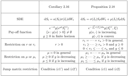
Recall the correspondence between the parameters in Corollary 2.16 and Proposition 2.18 given in Remark 2.12. In this section, we use the notation for the regime switching problem given Proposition 2.18. We summarise the conditions needed for Corollary 2.16 and Propo-sition 2.18 in Table 1 on page 37. The conditions in Table 1 are in addition to the common constraint σ₁2≤ · · · ≤σ2_n.

(38)

Both Corollary 2.16 and Proposition 2.18 can be applied to the American put problem in finite or infinite horizon. We examine this important case in Example 2.25 below.

Corollary 2.16 Proposition 2.18

SDE dSt=a(St)σ(It)dWt dSt=σ(It)StdWt+µ(It)StdSt

Pay-off function

e−rtg(eµtS_ts,i) e−R0tr(Iui)du_g₍_Ss,i t , Iti)

{s:g(s)>0} 6=∅ g(s,·) is increasing.

g≥0 in finite horizon g(·, i) is convex Restriction on r orri

r1 =· · ·=rn>0 in general.

r >0 r1 ≥ · · · ≥rn>0 andg≥0 0< r1 ≤ · · · ≤rn and g≤0 Restriction onµ orµi

µ= 0 in general µ1 =· · ·=µn in general

µ≥0 if gis decreasing µ1≥ · · · ≥µn ifg is decreasing

[image:38.612.69.493.124.377.2]

µ≤0 if g is increasing µ1 ≤ · · · ≤µn ifg is increasing Jump matrix restriction Condition (c1’) and (c2’) Condition (c1) and (c2)

Table 1: Comparison between Corollary 2.16 and Proposition 2.18

Remark 2.24. The monotonicity property of the value function not only offers us better understanding about the value function, but also has important practical implications for the numerical schemes used to estimate the value of the options.

Firstly, monotonicity results can reduce the complexity of numerical schemes. This point was noted in [2], where the authors also discussed the perpetual American put problem under the Regime Switching model. In infinite horizon, recall that the value function satisfies the free-boundary problem given in Remark 2.10. The numerical scheme proposed [39] tries to find stopping thresholds bi without assumptions on the ordering. By examining every possible arrangement, the problem has exponential complexity. However, u(s, i) ≥u(s, i0) implies bi < bi0. Hence, the problem has linear complexity in the number of states when

the monotonicity property is known.

Secondly, monotonicity results can be used to determine the validity of numerical schemes. In [12], Buffington and Elliott analysed the American put problem for two-state Regime Switching model in finite horizon. As discussed in Remark 2.11 (i), the stopping regions for finite horizon American put are characterised by stopping boundariesb1(t) and

b2(t). For a fixed time horizon T, the authors of [12] performed analysis on the value

(39)

also proposed a numerical scheme assuming this holds. This assumption is not a trivial one and it is unclear to us whether this always holds. Like in the perpetual case, monotonicity of the value function implies the monotonicity of stopping boundary. Hence, we know the algorithm in [12] can be used safely for some choices of parameters.

Example 2.25. Let u(s, i, T) be the value function of the American put option under Regime-Switching, i.e.,

u(s, i, T) = sup

0≤τ≤TE

e−

Rτ

0 r(I

i

t)dt₍_K−_Ss,i τ )+.

We want to know what are some sufficient conditions for u(·,1) ≤u(·,2) ≤ · · · ≤ u(·, n). Applying the result of Proposition 2.18 withg(s, i) = (K−s)+, we have

(i) σ1 ≤ · · · ≤σn,

(ii) r1 ≥ · · · ≥rn>0, (iii) µ1≥ · · · ≥µn.

(iv) The Q-matrix satisfies the coupling condition (c1) and (c2).

This result is consistent with one of the numerical examples in [15] and [42]. In their example,n= 4,T = 1, the parametersri’s andµi’s satisfy conditions (ii) and (iii), and the Q-matrix is given by



    

−3 1 1 1

1 −3 1 1

1 1 −3 1

1 1 1 −3



    

.

Applying Corollary 2.16 to gain function g(s) = (K−s)+, we have (i’) σ1 ≤ · · · ≤σn,

(ii’) r1 =· · ·=rn>0, (iii’) µ1=· · ·=µn>0,

(iv’) The time changed Q-matrix satisfies the coupling condition (c1) and (c2).

Condition (iii’) is somewhat restrictive, but Corollary 2.16 can be used to improve condition (iii’) by a simple transformation. LetSt be of the form

S_ts,i=sexp

Z t

0

σ(Iu)dWu+c

Z t

0

σ(It)2dt

On properties of the American put option under several models

warwick.ac.uk/lib-publications

A Thesis Submitted for the Degree of PhD at the University of Warwick

Permanent WRAP URL:

http://wrap.warwick.ac.uk/95313

Copyright and reuse:

This thesis is made available online and is protected by original copyright.

Please scroll down to view the document itself.

Please refer to the repository record for this item for information to help you to cite it.

Our policy information is available from the repository home page.

On properties of the American put

option under several models

by

Yufan Zhao

1164727

A thesis submitted in partial fulfilment of the requirement for

the degree of

Acknowledgements

Declarations

Contents

1

Introduction and Preliminaries

2

On Optimal Stopping under Regime-Switching and

Re-lated Models