Single nanoparticle electrochemistry

(1)

warwick.ac.uk/lib-publications

A Thesis Submitted for the Degree of PhD at the University of Warwick Permanent WRAP URL:

http://wrap.warwick.ac.uk/99424/

Copyright and reuse:

This thesis is made available online and is protected by original copyright. Please scroll down to view the document itself.

Please refer to the repository record for this item for information to help you to cite it. Our policy information is available from the repository home page.

(2)

Single Nanoparticle Electrochemistry

By

Minkyung Kang

Thesis

Submitted to the University of Warwick

for the degree of

Doctor of Philosophy

Supervisor: Prof Patrick R. Unwin

Department of Chemistry

(3)

List of Figures

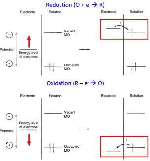
Figure 1.1 Illustration of a reduction (top) and oxidation (bottom) process, occuring between two different redox molecules in solution and an electrode. The oxidised and

reduced forms of each molecule are represented as “O” and “R”, respectively. The

highest occupied molecular orbital (HOMO) of the molecule is denoted “Occupied

MO” and lowest unoccupied molecular orbital (LUMO) is denoted “Vacant MO”.

Figure 1.1 was adapted from Bard and Faulkner (2001).1_{... 2}

Figure 1.2 Pathway of a general electrode reaction. It needs to be noted that there are redox species limited by mass transfer [e.g., Hexaammineruthenium (III/II)] rather

than other processes described in Figure 1.2. Figure 1.2 was adapted from Bard and

Faulkner (2001).1... 3

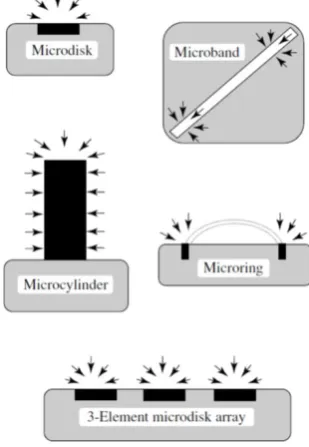
Figure 1.3 Most commonly utilised microelectrode geometries and their associated diffusion field. Figure 1.3 was adapted from Bard et al. (2003).8 ... 9

Figure 1.4 Schematic representation of the diffusion profiles on a disk-UME at (A) short (linear diffusion profile) and (B) long (radial diffusion profile) timescales. Figure

1.4 was adapted from Bard et al. (2003).8... 11

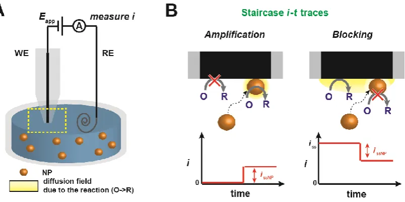
Figure 1.5 (A) Schematic of a SNEI experiment setup using a UME as the WE. (B) Schematics and typical i-t transient arising from NPs after a “sticking” impact (i.e., “staircase” response), resulting in either amplification (left) or blocking (right) of the

reaction of interest on the collector electrode surface. ... 13

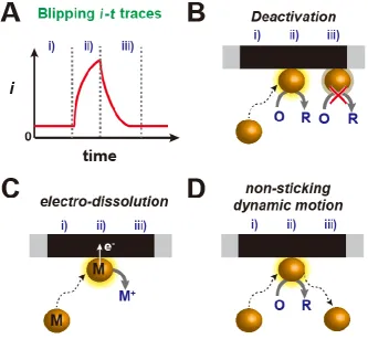
Figure 1.6 (A) Schematic of a typical i-t transient for a “blipping” response during a SNEI experiment. Three possible processes giving rise to the response are illustrated:

(B) deactivation; (C) electrodissolution; and (D) non-sticking dynamic motion. ... 16

Figure 1.7 (A) A schematic of the early stage of micro-droplet electrochemical cell setup with optical and contact force monitoring. (B) Optical image of a glass capillary

with an applied silicone gasket. Figure 1.7 was adapted from Lohrengel et al. (2001).67

(8)

Figure 1.8 (A) Schematics of the micro-droplet electrochemical cell setup for SNEI experiments using a single channelled probe (left)24,51 and a double channelled probe

(right).44,76,77 Confined droplet contact on the substrate is achieved through monitoring

signals (i.e., currents) induced by the circuit completion (isub) and the deformation of

the droplet (iDC). More operation details are provided in Section 1.3.4. (B) Principle

of a single Au NP electrochemical impact on SAM-modified Au electrodes and typical

i-t responses with, −OH, −COOH, and −CH3 terminated SAMs. (B) was adapted from

Chen et al. (2015).77_{(C) Illustration of an AuO}

x layer formation on an Au NP through

electron tunnelling between the Au NP and passivated Au electrode surface, with a

typical i-t response of the process followed by comparisons of size analysis between

TEM analysis and SNEI. (C) is adapted from Bentley et al. (2016).24 ... 22

Figure 1.9 it as a function of tip–substrate separation, L (dt-s normalised with rtip)

where the substrate is (A) a conductor (“positive feedback”) and (B) an insulator

(“negative feedback”), with illustrations of the diffusion profile at the tip in each case,

in bulk (hemispherical), on a conductor (feedback) and on an insulator (hindered).

Figure 1.9 was adapted from Bard et al. (2012).82 ... 25

Figure 1.10 Approach curves as a function of k0 for electron transfer (redox) reaction at the substrate. From top to bottom, k0 (cm s-1) is (a) 1, (b) 0.5, (c) 0.1, (d) 0.025, (e) 0.015, (f) 0.01, (g) 0.005, (h) 0.002, and (i) 0.0001. Curve (a) is identical to that for

mass transfer controlled (electrochemically reversible) reaction and curve (i) for an

insulating substrate in Figure 1.9. Figure 1.10 was adapted from Bard et al. (2012).82

... 25

Figure 1.11 (A) Schematic showing the basic principles of AFM operation and (B) force-ds-t relationships at approach and retract of the AFM tip. (C) Optical and

scanning electron microscopic (SEM) images of manually fabricated Pt wire

SECM-AFM probe. (C) was adapted from Macpherson et al. (2000).97 (D) Principle of the

SECM-AFM technique for the interrogation of PEGylated ferrocene (PEG =

polyethyleneglycol) anchored on individual gold NPs (left). Simultaneously obtained

topography and tip current images (right). Cross sections of the topography and tip

current images (dotted white lines) are respectively plotted in red and blue.

(9)

in the plots) are plotted as black traces. (D) was adapted from Huang et al. (2013).106

... 28

Figure 1.12 (A) Basic principle of SICM operation, where a potential bias between two QRCEs and the induced ionic current is noted as ΔV and iion, respectively. (B) iion

-ds-t relationship during approach of a SICM probe to a surface. The magnitudes of iion

begins to decrease where ds-t is similar to the diameter of the probe (dtip). ... 29

Figure 1.13 (A) Schematic illustration of double-channelled SECM-SICM probe fabrication (top) with optical (bottom left) and SEM (bottom right) images of the

probes. (A) was adapted from Takahashi et al. (2011).119 (B) Schematic showing the

basic principles of SECM-SICM operation. (C) (i) A SEM image of spherical Pt NPs

electrochemically decorated on a GC surface and (ii) corresponding topography and

ORR reactivity maps of the surface, simultaneously obtained by the SECM-SICM

technique. (C) was adapted from O’Connell et al. (2014).121_{... 30}

Figure 1.14 (A) Basic operating principle for electrochemical reaction mapping with SICM. (B) Cyclic voltammograms acquired from the substrate (Pt UME, red) and

concurrently monitored current at the SICM probe (blue) which is positioned at the

central part of the substrate electrode during the potential sweep. (C) Topography (left)

and reactivity (middle, HER; right, hydrazine oxidation) maps obtained from dynamic

reaction imaging with SICM. Figure 1.14 was adapted from Momotenko et al. (2016).116 ... 32

Figure 1.15 (A) Schematic of the SECCM setup, with a TEM image of a double-chanelled quartz nanopipette (dtip ≈ 100 nm) inset. (B) Approach curves of an SECCM

probe with idc and iac as a function as z extension towards the substrate. Shown above

the plots are illustrations delineating three regions; in air, where no contact has been

made with the substrate; jump-to-contact (dashed line); and contact. Figure 1.15 was

adapted from Mirkin and Amemiya (2015).139 ... 35

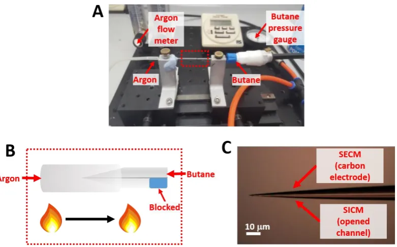
Figure 2.1 (A) A photograph and (B) schematic depicting the experimental set up for the butane pyrolysis process during fabrication of double-channelled SECM-SICM

(10)

Figure 2.2 Electron microscopy images of the nanopipette probes used for high-resolution electrochemical imaging. (A) SEM image of a double-channelled theta

nanopipette. (B) TEM image of a single-channelled nanopipette. Figure 2.2 was

adapted from Kang et al. (2016).6 ... 52

Figure 2.3 Photograph of nanopipette probes mounted on a brass holder for TEM characterization. ... 52

Figure 2.4 Schematic of a typical SEPM set up, for use with the WEC-SPM software. (A) Illustrates the positioning system and (B) shows the general control of the SEPM

system. Figure 2.4 was adapted from the WEC-SPM Control Software User Guide

(2017).8 ... 53

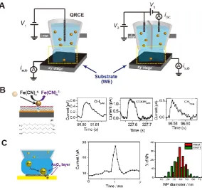
Figure 3.1 RuOx NP landing experiments in an ultramicro-electrochemical cell,

showing the cell setup (top), with a typical theta pipet for meniscus contact and NP

delivery to a working electrode (HOPG) substrate. There is no oxidation of H2O2 at

the HOPG electrode surface, i.e., no surface current (isurf), as shown on the bottom left,

unless a NP impacts with the surface and sets off the electrocatalytic oxidation of

H2O2 at the NP (bottom right). ... 59

Figure 3.2 Cyclic voltammograms, with and without H2O2 present, on HOPG in 0.1

M phosphate buffer (pH 7.4) at a scan rate of 0.1 V s-1. ... 61

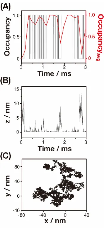
Figure 3.3 (A) Comparisons of the occupancy (black) and the average occupancy of the NP considering the experimental conditions (red). (B) The height (z) of the NP

above the collector electrode during the interaction of a NP with the collector electrode

and (C) lateral trajectory of the NP. ... 64

Figure 3.4 (A) FE-SEM and (B) TEM images of RuOx NPs synthesized with sodium citrate. (C) Size distribution from the analysis of TEM images (red) and from DLS

(green), in terms of the particle radius, rNP. ... 66

Figure 3.5 SEM images of RuOx NPs synthesized without sodium citrate. ... 66

Figure 3.6 Current responses of RuOx NP impacts at HOPG in the presence of 0.5

(11)

synthesized (A) without or (B) with a sodium citrate capping step. Note the difference

in the current scales. ... 67

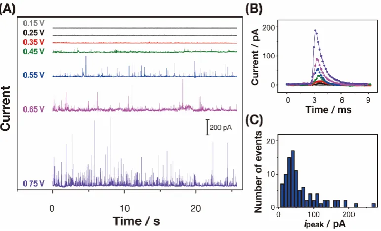
Figure 3.7 (A) Current (isurf) responses for 0.5 mM H2O2 oxidation with 15 pM

RuOxNPs in 0.1 M phosphate buffer solution (pH 7.4) at different Eapp at the HOPG

collector electrode (0.15 V, 0.25 V, 0.35 V, 0.45 V, 0.55 V, 0.65 and 0.75 V vs

Ag/AgCl QRCE). (B) Example current responses of individual impacts of RuOxNPs

at the different Eapp with the color matched with part A; the bigger the current

magnitude the higher the Eapp. (C) Distribution of peak currents, ipeak, from collision

experiments at 0.55 V. ... 68

Figure 3.8 Comparison of current responses in RuOx NP landings with 0.5 mM H2O2

and without 0.5 mM H2O2 at 0.55 V. ... 68

Figure 3.9 Plot of average ipeak against different Eapp from Figure 3.7. ... 69

Figure 3.10 Histograms of the rise time from (A) 200 simulations and (B) 16 experimental transients. Experimental i–t traces (blue lines) are presented in parts C

and D. These are the average (one standard deviation) of (C) 10 individual transients

that had a rise time of 330 μs and (D) 5 individual traces that had a rise time of 500 μs. Shown alongside are simulated occupancy traces (black lines), which displayed a

similar rise time for comparison. ... 70

Figure 3.11 Typical multiple RuOx NP impact events at a collector electrode potential of 0.55 V. ... 73

Figure 4.1 Schematic of the set up for SECCM NP impact experiments. ... 83

Figure 4.2 Representative TEM images of Ag NPs with nominal diameters of (a) 10 nm, (b) 20 nm, (c) 40 nm, (d) 60 nm and (e) 100 nm (abbreviated as Ag10NPs,

Ag20NPs, Ag40NPs, Ag60NPs and Ag100NPs, respectively). ... 86

Figure 4.3 Linear sweep voltammogram (LSV) (100 mV s-1_{) for the reduction of 2}

mM Ru(NH3)63+ in 0.1 M KNO3 solution by the meniscus contact on GC using a glass

pipette (diameter of 8 m) and SEM image of the footprint after the meniscus contact

(12)

Note that the LSV is not fully at steady-state due to the scan speed used and the fact

that SECCM diffusion is from a conical segment rather than fully hemispherical. .. 87

Figure 4.4 Representative I-t transients obtained during the polarization at E= +0.6 V vs Ag/AgCl of a (a) Au UME, (b) CF-UME and (c) GC electrode in SECCM setup, with different amplification time constants. d) Peak to peak background current vs amplification time constant for different electrode materials and setups. ... 89

Figure 4.5 Representative current transients obtained by applying E = +0.6 V vs Ag/AgCl to a GC electrode with a solution containing Ag NPs with nominal diameter

of (a) 10 nm and (b,c) 20 nm. The numbers i-v refer to different cases discussed in the

text. ... 91

Figure 4.6 Representative current transients obtained by applying E = +0.6 V vs Ag/AgCl to a GC electrode with a solution containing Ag NPs with nominal diameter

of (a, b) 40 nm and (c, d) 60 nm. The numbers i-v refer to different cases discussed in

the text. ... 92

Figure 4.7 Representative current transients obtained by applying E = +0.6 V vs Ag/AgCl to a (a, b) GC and a (c, d) Au electrode with a solution containing Ag NPs

with nominal diameter of 100 nm. The numbers i-v refer to different cases discussed

in the text. ... 94

Figure 4.8 (a) Log-log plot of the charge histograms for single events recorded during the stripping of Ag NPs with nominal diameter of 10, 20, 40, 60 and 100 nm on GC

and 100 nm Ag NPs on Au electrodes. Histograms of the (b) equivalent NP diameter

(assuming dissolution of whole NP), (c) event duration and (d) maximum current. . 96

Figure 4.9 Log-log plot of the event duration histograms for single events recorded during the stripping of Ag NPs with nominal diameter of 10, 20, 40, 60 and 100 nm

on GC and Au electrodes. ... 98

Figure 4.10 Log-log plot of the maximum current histograms for single events recorded during the stripping of Ag NPs with nominal diameter of 10, 20, 40, 60 and

(13)

Figure 4.11 (a) LSV (50 mV s-1_{) for Ag (UME of diameter = 125} m)

electrodissolution in presence (black) and absence (red) of 1 mM trisodium citrate in

25 mM NaNO3. (b) Current-time curves at different applied potentials (Eapp vs.

Ag/AgCl) where the steady-state currents are corresponding to 0.6 (black), 1.3 (blue),

and 1.9 (red) mM of Ag+_{concentrations on the Ag UME surface. Citrate inhibits Ag}

electrodissolution (probably by surface adsorption) but there is no evidence of surface

passivation due to Ag3Cit precipitation... 101

Figure 4.12 Log-log plot of the time elapsed between consecutive events recorded during the stripping of Ag NPs with nominal diameter of 10, 20, 40, 60 and 100 nm

on GC and Au electrodes. The blue dashed line represents the estimated average time

between two events if each NP was fully stripped in one single event. ... 104

Figure 4.13 Representative current transients obtained with (a) τC = 100 s and (b) τC

= 5 ms, by applying E=+0.6 V vs Ag/AgCl to a GC electrode with a solution

containing Ag NPs with nominal diameter of (left) 40 nm and (middle) 100 nm, and

to a Au electrode with a solution containing Ag NPs with nominal diameter of 100 nm

(right). Histograms of (c) equivalent NP diameter (assuming complete dissolution of

NPs) and (d) event duration, both for τC = 5 ms. ... 106

Figure 4.14 Schematic of different processes of electrochemical dissolution of Ag NPs with nominal diameters of (a) 10, (b) 20, 40 and (c) 60, 100 nm... 108

Figure 4.15 Representative periodic I-t transients obtained by applying E=+0.6 V vs Ag/AgCl to a GC with a solution containing Ag NPs with nominal diameter of (a,b)

40 nm and (c,d) 60 nm, and to Au with a solution containing Ag NPs with nominal

diameter of (e,f) 100 nm... 111

Figure 4.16 Periodic I-t patterns (from Figure 4.15) and Schematic representation of the electrochemical dissolution mechanism of Ag NPs on a (a) GC and on (b) Au

substrate... 112

Figure 5.1 (A) A 2D Schematic representation of the FEM simulation domain with boundary descriptions shown in Table 5.1. All other boundaries not explicitly labeled

were set as no flux boundaries. (B) Simulated I-V curved with varying surface charge

(14)

for reaction mapping experiments, with the nanopipette positioned in bulk solution.

Note that the geometry of the nanopipettes were consistent according to the TEM

characterization of multiple nanopipettes, and the average current magnitude at Vtip of

+0.15 V yielded 188 pA with a standard deviation of 7 pA (N = 4). (C) Simulated

SICM approach curve (tip-substrate separation versus normalized Itip) with the

solution conditions as in the experiments. ... 124

Figure 5.2 Transmission electron microscopy (TEM) image of a representative nanopipette with a tip diameter of approximately 30 nm. ... 125

Figure 5.3 (A) Schematic of the experimental setup used for simultaneous topographical/electrochemical mapping of a substrate electrode using SICM. (B)

Shown at the top are schematics of the main features of the imaging procedure during

the hop motion of the probe (numbered 1 to 4) at each pixel. A trace of z-position and

Vsub during each step is shown at the bottom. The overall procedure can be summarized

as follows: (1) approach towards the substrate surface under DC ionic current feedback

to reach the set point distance; (2) small retract (“small lift-up”); (3) waiting time of

20 ms followed by potential step by jumping Vsub from Vsub1 to Vsub2; and (4) full retract

before the hop procedure is repeated at the next pixel, typically 20 nm lateral

displacement from the previous one. The tip current, measured throughout, was

analyzed as discussed in the text. ... 127

Figure 5.4 (A) Plots of z-position (black trace) and substrate electrode potential (Vsub)

(blue trace) vs. time, showing the protocol utilized during each hop (pixel-level

measurement) of a typical imaging experiment. (B) The corresponding tip current (Itip)

vs time plot, recorded simultaneously with (A). ... 128

Figure 5.5 LSVs (potential sweep at Vsub) obtained at two individual Au UMEs

(diameter ≈ 10 m) in a solution containing 3 mM NaBH4 and 30 mM NaOH with

scan rate of 0.2 V s-1_{. The substrate current (I}

sub) and tip current (Itip) were concurrently

measured at fixed tip bias potentials (Vtip) of (A) +0.15 V and (B) -0.35 V. The SICM

probe was positioned at the center of the Au UME at a vertical distance of 26 nm (vide

infra) during the measurements. For normalization, the magnitude of Itip without the

substrate reaction was (A) 180 pA and (B) -850 pA. (C) Schematics (not to scale)

(15)

nanopipette at positive (left) and negative (right) tip biases during BH4- oxidation.

... 132

Figure 5.6 FEM simulations of normalized Itip at different fixed biased potential at the

tip (Vtip) with an increase in k at the substrate, showing higher sensitivity of Itip to the

reaction at positive Vtip in correspondence with the experimental results in Figure 2A

and B of the main manuscript. ... 133

Figure 5.7 FEM simulation results of OH-_{concentrations near the end of the}

nanopipette and above a reactive substrate at biased potential at the tip (Vtip) of + 0.15

V (A and B) and -0.35 V (C and D) with ‘slow’ and ‘fast’ substrate reaction, defined

by k = 70 cm4 mol-1 s-1 and k = 1.2106 cm4 mol-1 s-1 respectively. Corresponding total

ionic concentrations shown in E-H. ... 134

Figure 5.8 (i) SICM topography and (ii) electrochemical activity maps of an Au UME (diameter ≈ 10 m), obtained simultaneously, in a solution containing 3 mM NaBH4

and 30 mM NaOH, recorded with Vsub2 = 0.9 V, Vtip = +0.15 V and ds-t values of (A)

11 nm, (B) 26 nm and (C) 106 nm. There is no interpolation of the data and each of

the images contains 1681 pixels. ... 136

Figure 5.9 (i) SICM topography and (ii) electrochemical activity maps of a segment of an Au UME (diameter ≈ 10 m) sealed in glass, obtained in a solution containing

3 mM NaBH4 and 30 mM NaOH, recorded with dt-s = 26 nm, Vtip = +0.15 V and Vsub2

values of (A) 0.3 V and (B) 0.6 V. There is no interpolation of the data and the images

contain 1681 pixels. ... 137

Figure 5.10 (A) Cyclic voltammograms (CVs) obtained at Au (diameter ≈ 10 m, red

trace) and CF (diameter ≈ 7 m, black trace) UMEs in an aqueous solution containing

3 mM NaBH4 and 30 mM NaOH with a scan rate of 0.2 V s-1. (B) SICM topography

map and (C) corresponding electrochemical activity image, obtained at the CF UME

in the solution defined above with dt-s = 26 nm, Vtip = + 0.15 V and Vsub2 = 0.9 V,

showing the inactive carbon surface for BH4- electro-oxidation. The topography map

of the UME shows that the CF (red) extends from the end of the glass support (blue),

arising from the polishing process during UME fabrication/conditioning. There is no

(16)

Figure 5.11 (A) SEM images of Au nanostructures on a CF UME: (i) an electron micrograph of the CF UME with deposited Au nanostructures and (ii) magnified view

of the red box in (i), indicating the area imaged with SICM. (B) (i) SICM topography

map and (ii) corresponding electrochemical activity image of Au nanostructures at

Vsub2 = 0.65 V. (iii) is a replotted electrochemical image of selected area in Figure

5.11B (ii); with the scale bar indicating 100 nm. (C) is identical to (B), except the data

were obtained at a Vsub2 of 0.9 V. Data were obtained in a solution containing 3 mM

NaBH4 and 30 mM NaOH at Vtip of +0.15 V, recorded with a ds-t value of 26 nm (when

the nanopipette is positioned above the top of the particle). There is no interpolation

of the data and the full SICM images each contain 3111 pixels in total. Note that the

SICM image shows the CF to protrude from the glass surround (raised areas in the left

of the topographical images). ... 140

Figure 5.12 (A) SEM images of AuNPs on a CF UME: (i) a full picture of the CF UME with AuNPs and (ii) a magnified view of the red box in (i), indicating the area

scanned with SICM. (B) Annotation of individual NPs from the SEM map and (C) corresponding topographical SICM data (pixel density: 2600 pixels m-2_{) in a solution}

containing 3 mM NaBH4 and 30 mM NaOH at a Vtip of +0.15 V. There is no

interpolation of the data and the SICM image contains 3136 pixels. ... 141

Figure 5.13 (A) SEM images of AuNPs on a CF UME, shown in the main manuscript, Figure 5. (B) A representative TEM image of the cross-section of a single AuNP. The

TEM samples were prepared using FIB-SEM from the sample shown in (A). ... 142

Figure 5.14 (i) SICM topography maps and (ii) simultaneously recorded activity images of AuNPs on a CF UME (diameter = 7 m) (pixel density: 2600 pixels m-2_),

obtained in a solution containing 3 mM NaBH4 and 30 mM NaOH, at Vsub2 values of

(A) 0.65 V, (B) 0.75 V, (C) 0.9 V and (D) 0.95 V. During mapping, Vtip and ds-t were

fixed at +0.15 V and 26 nm, respectively. There is no interpolation of the data and the

images contain 3136 pixels. ... 143

Figure 5.15 CVs obtained at (A) a CF UME (diameter ≈ 7 m) and (B) a CF UME with electro-deposited AuNPs (Figure 5.12A) in a solution containing 3 mM NaBH4

and 30 mM NaOH with a scan rate of 0.1 V s-1. The CVs were obtained before the

(17)

avoid surface oxidation/reduction of Au, which would modify the surface of the

AuNPs.59 ... 144

Figure 5.16 (A) Array of NPs on surface separated by distance Sep. (B) Effect of separation distance on predicted normalized current above the central particle. (C) OH-

concentration along the bottom plane of the simulation domain showing little overlap

between the particles when separated by 1 m. (D) OH- _{concentration along the bottom}

plane of the simulation domain showing a strong overlap between the particles when

separated by 0.17 m. The value of k was 2.4104 cm4 mol-1 s-1 in each simulation. ... 145

Figure 5.17 FEM simulations of an isolated NP with BH4- oxidation at two different

heterogeneous rate constant (k) (i.e. 3.4103_cm4_mol-1_s-1 (low) and 1.2106_cm4_mol -1_s-1_{(high)). Total ion concentration profiles (A and B) showing how the ion}

concentration around a NP (and at the end of the tip) changes with the reaction rate.

(C and D) predicted tip current profiles around the NP showing the same ring effect

observed experimentally at low k, in particular. (E and F) show simulated tip current

versus radial direction profiles with the nanopipette tracing the NP or substrate at a distance corresponding the approach current threshold and the small lift up (i.e. 26 nm

when over the particle centre) at low and high k, respectively. (C-F) highlight the ‘ring

effect’ in the activity around the NP, notably at low k... 147

Figure 6.1 Fabrication of dual-barrel nanoprobes for use in SICM-SECM. (a) Carbon was deposited in one barrel of the probe via the pyrolysis of butane (SECM) while the

other was kept open (SICM). Inset transmission electron microscopy (TEM) images

show an example of both complete (left) and incomplete (right) carbon deposition.

Scale bar in both micrographs is 500 nm. (b) The probe diameter was regulated using

focused ion beam (FIB) milling. Inset TEM images show a probe with scale bars of 5

μm (left) and 500 nm (right) after FIB milling. ... 158

Figure 6.2 Schematic (not to scale) of a 2D slice from the 3D FEM simulation of a dual-channel nanopipette above a surface of variable uptake rate constant, k. Boundary

(18)

Figure 6.3 Difference in the simulated SICM current at a probe-substrate separation distance (d, see above) of 120 nm over substrates of differing uptake rates when

compared to the SICM current at 120 nm over a surface with an uptake rate constant

of 0 cm s-1. ... 163

Figure 6.4 Comparison between approach curves in both the SICM and SECM channels from FEM simulations and from a typical experimental approach. In both

figures the zero point is that taken from the simulations where the probe-substrate

separation is known precisely. The experimental approach curves have been shifted

by 120 nm from the point of closest approach. ... 164

Figure 6.5 SICM-SECM experimental setup for the investigation of cellular uptake. (a) The current flowing between two Ag/AgCl QRCEs, one in bulk and one in the

open channel of the probe, with an applied bias, V1, used for topographical feedback

in an SICM configuration. The carbon electrode used to measure the local

concentration of the species is at a bias V2 - V1. (b) Schematic showing the

diffusion-migration of [Ru(NH3)6]3+ from the SICM barrel into the near cell region. The current

due to the reduction of [Ru(NH3)6]3+ at the SECM channel is monitored on approach

of the probe to the surface and compared to the steady-state bulk current response to

quantify uptake rates. It should be noted that transport via an ion channel is just one

of many possible membrane transport mechanisms and is depicted herein for

illustrative purposes. ... 167

Figure 6.6 Finite element method (FEM) modeling of the SICM-SECM uptake system. (a) Simulated SICM approach curve (current vs. distance) to a surface of zero

uptake with a probe of the same geometry as used experimentally, with

electrochemistry switched on at the SECM channel. The current data are plotted as the

percentage drop in ionic current from the bulk value (~850 pA). The experimental

threshold (red line in (a)) was used to determine a working distance at which

steady-state simulations (b) were carried out to calibrate the normalized SECM current as a

function of the uptake rate constant at the surface. The normalized SECM current is

the value at d = 120 nm divided by that with the probe in bulk solution (~10 pA). (c)

and (d) show the concentration of [Ru(NH3)6]3+ at steady state with initial

(19)

Figure 6.7 SICM-SECM topographical and [Ru(NH3)6]3+ uptake mapping of a Zea

mays root hair cell on a glass substrate. (a) Optical image of the scanned root hair cell (A) on a glass support with the end of the probe also visible (B); scan area denoted by

the dashed rectangle. (b) Substrate topography extracted from the z-position at the

point of closest approach. (c) Normalized SECM current map showing the difference

in uptake between glass substrate (zero uptake) and the root hair cell. ‘Normalized

current’ is the ratio of the [Ru(NH3)6]3+ steady-state limiting reduction current at the

point of closest approach to the reduction current in bulk. Individual experimental

approach curves from the scan in (c) are shown in (d), at the four positions numbered.

SICM (e) and SECM (f) currents across the entirety of the scan (400 separate approach

curves) demonstrate minor current drift for SICM, but some effect for SECM, making

the self-referencing approach essential. The red line in (f) shows the trend in bulk

SECM current, ignoring the approaches to either the cell or the glass. ... 173

Figure 6.8 SICM-SECM topographical and [Ru(NH3)6]3+ uptake mapping of two

regions of a single Zea mays root hair cell. (a) Optical image of the scanned root hair cell; scan area denoted by the dashed rectangle. (b) Substrate topography extracted

from the z-position at the point of closest approach from the SICM channel. (c)

Normalized SECM current map showing a clear difference in uptake between the root

hair cell body (higher current, lower uptake) and the root hair cell tip (lower current,

higher uptake). ‘Normalized current’ is the ratio of the [Ru(NH3)6]3+ reduction current

at the point of closest approach to the same reduction current in bulk. (d) Histograms

of the normalized SECM current across the two different regions of the root hair cell,

‘tip’ and ‘body’ (see (b)). ... 175

Figure 6.9 Raw data normalized current image of the root hair cell scan presented in

(20)

List of Tables

Table 2.1 Capillary materials, dimensions, suppliers and the pulling parameters of the pipettes utilised in each chapter. ... 49

Table 2.2 The BNC channels from the breakout box (AO = Analog Output, AI = Analog Input). ... 55

Table 3.1  -potential measurements of RuOx NPs with or without the sodium citrate

capping step. ... 66

Table 4.1 Summary of Conditions for previous studies of Ag NP electro-oxidation. ... 81

Table 4.2 Average diameters (nm) of Ag NPs as determined from TEM and DLS (in absence and presences of 25 mM NaNO3). ... 86

Table 4.3 Estimated concentration, diffusion coefficient and impact frequency of distributions of Ag NPs with nominal diameters of 10, 20, 40, 60 and 100 nm. ... 87

Table 5.1 FEM boundary conditions for simulation geometry depicted in Figure 5.1. ... 125

Table 5.2 Comparison of size analysis results between SEM and SICM from Figure 5 in the main manuscript: NP numbers are annotated in Figure 5B. The particle boundary

in SICM topographical data to create Table S2 was defined as a height threshold of 10

nm above the support electrode... 142

Table 6.1 Diffusion coefficients of the species simulated. ... 161

Table 6.2 Boundary conditions for the FEM model with boundaries corresponding to Figure 6.2 below. ... 162

Table 6.3 Normalized SECM current values at the distance of closest approach from a series of approach curves to a Zea mays root hair cell at different approach rates. Each value given is the mean of three approaches and an error of one standard

(21)

Abbreviation

ac Alternating current

AFM Atomic force microscopy

Cd Double layer capacitance

CE Counter electrode

CF Carbon fibre

Cstray Stray capacitance

CV Cyclic voltammogram

dc Direct current

EOF Electroosmotic flow

ET Electron transfer

FEM Finite element method

FE-SEM Field emission-scanning electron microscopy

FIB Focused ion beam

FPGA Field-programmable gate array

GC Glassy carbon

HER Hydrogen evolution reaction

HOPG Highly oriented pyrolytic graphite

LSV Linear sweep voltammogram

MSE Mercury sulfate electrode

NP Nanoparticle

ORR Oxygen reduction reaction

Pd-H2 Palladium wire saturated with hydrogen

PZC Potential of zero charge

QRCE Quasi-reference counter electrode

RAM Random assembly microelectrode

RE Reference electrode

RuOx Ruthenium oxide

SAM Self-assembled monolayer

SCE Standard calomel electrode

(22)

SECM Scanning electrochemical microscopy

SEPM Scanning electrochemical probe microscopy

SERS Surface-enhanced Raman scattering

SICM Scanning ion conductance microscopy

SNEI Single nanoparticle electrochemical impact

SWCNT Single-wall carbon nanotube

TEM Transmission electron microscopy

UME Ultramicroelectrode

(23)

Acknowledgements

Firstly, I would like to thank my supervisor Prof Patrick R. Unwin for all of

his support, encouragement and enthusiasm throughout my PhD. He has given me so

many opportunities to develop my scientific skills and knowledge here in Warwick

Electrochemistry and Interfaces Group and his advice on research and general life

have brought me here to finalise my PhD.

I have truly enjoyed working with the state-of-art electrochemical

instrumentation and with the amazing people in the group. I would like to thank all of

you who has been in the group (including visitors) throughout my PhD. I sincerely

appreciate your expertise and kindness, which has been incredibly helpful for me.

Special thanks to “Team Cell” including Binoy (previous member), David and

Ashley for being fantastic to work with and, more importantly, great friends to throw

banter at each other. I also would like to acknowledge Faduma, Maria, Emma and Sze

who has been through the same years with me in this group and provided “supportive”

talks during coffee breaks. Special thanks to Faduma, for introducing me to a great

“field” of dank memes. Among the amazing master students who have worked with

me in the group, I would like to give special thanks to Erin, who taught me how

incredible it is to work with someone so positive and energetic. Also, thanks to all the

lads in the group who had a few “Dangerous Wednesday” sessions alongside me and

endured drunk MK.

I appreciate support from my parents from South Korea and my lovely sister,

Minjung, who visited me in England and spent great time with me here. Finally, a

huge thank you to Cameron, who has been the best supporter during my PhD at work

and in life and put up with my everyday craziness.

Finally, I acknowledge the University of Warwick Chancellor's International

(24)

General Declaration

The work presented in this thesis is entirely original and my own work, except where

acknowledged in the list below. I confirm that this thesis has not been submitted for a

degree at another University. Material from this thesis has been published, as noted

below.

The material in Chapter 3 was published as:

Time-Resolved Detection and Analysis of Single Nanoparticle Electrocatalytic Impacts

Minkyung Kang, David Perry, Yang-Rae. Kim, Alex W. Colburn, Robert A. Lazenby, Patrick R. Unwin

J. Am. Chem. Soc. 2015, 137 (34), 10902–10905. 3D random walk simulation in the material was performed by Dr. David Perry

Electrochemical Dissolution via Silver Single Silver Nanoparticle Impacts: Morphological Analysis of the Dynamic Response

Jon Ustarroz†, Minkyung Kang†, Erin Bullions, Patrick R. Unwin

Chem. Sci. 2017, 8, 1841–1853. (†equally contributed) The data analysis and presentation in the material were performed with Dr. Jon Ustarroz.

Simultaneous Topography and Reaction Flux Mapping At and Around Electrocatalytic Nanoparticles

(25)

ACS Nano 2017, 11 (9), 9525-9535. Finite element method (FEM) simulations in the material were performed by Dr. David Perry and characterization of nanoparticles with

transmission electron microscopy (TEM) was performed by Dr. Geoff West.

The material in Chapter 6 was submitted as:

Quantitative Visualization of Molecular Delivery and Uptake at Living Cells with Self-Referencing Scanning Ion Conductance Microscopy-Scanning Electrochemical Microscopy

Ashley Page, Minkyung Kang, Alexander Armitstead, David Perry, Patrick R. Unwin Anal. Chem. 2017, 89, 3021−3028. The material in this paper also provided the basis

of a chapter in Ashley Page’s thesis (Warwick, expected in 2017) who jointly

performed the experiments and fully performed FEM simulations. The substrate

samples (e.g., corn roots) were prepared by both Ashley Page and Mr. Alexander

Armitstead.

Additionally, during my PhD I have contributed to the following papers whose results

are not presented in this thesis:

Electrochemical maps and movies of the hydrogen evolution reaction on natural crystals of molybdenite (MoS2): basal vs. edge plane activity

Cameron L. Bentley, Minkyung Kang, Faduma M. Maddar, Fengwang Li, Marc Walker, Jie Zhangb Patrick R. Unwin

Chem. Sci. 2017, 8, 6583-6593.

Time-Resolved Detection of Surface Oxide Formation at Individual Gold Nanoparticles: Role in Electrocatalysis and New Approach for Sizing by Electrochemical Impacts

(26)

J. Am. Chem. Soc. 2016, 138 (39), 12755–12758.

Characterization of Nanopipettes

David Perry, Dmitry Momotenko, Robert A Lazenby, Minkyung Kang, Patrick R. Unwin

Anal. Chem. 2016, 88 (10), 5523–5530.

Simultaneous Interfacial Reactivity and Topography Mapping with Scanning Ion Conductance Microscopy

Dmitry Momotenko, Kim McKelvey, Minkyung Kang, Gabriel N. Meloni, Patrick R .Unwin

Anal. Chem. 2016, 88 (5), 2838–2846.

High-Speed Electrochemical Imaging

Dmitry Momotenko, Joshua C. Byers, Kim McKelvey, Minkyung Kang, Patrick R. Unwin

ACS nano 2015, 9 (9), 8942–8952

And two review articles, which discusses much of the work published in this thesis

and the above-mentioned studies:

Scanning Electrochemical Cell Microscopy: New Perspectives on Electrode Processes in Action

(27)

Frontiers in Nanoscale Electrochemical Imaging: Faster, Multifunctional, and Ultrasensitive

Minkyung Kang,† Dmitry Momotenko,† Ashley Page,† David Perry,† Patrick R. Unwin,

(28)

Abstract

This thesis presents various pipette-based techniques for resolving the electrochemical

activities of single nanoentities (e.g., nanoparticles, NPs) in time and/or space. In

particular, the work provides a framework for understanding the (electro)chemistry of

single NPs and the development of tools to resolve them temporally and/or spatially.

Through the use of the state-of-the-art instrumentation developed by the Warwick

Electrochemistry & Interfaces Group (WEIG), electrochemical measurements with a

“static” probe (i.e., micro-droplet electrochemical cell) have revealed detailed

(temporally-resolved) information on the dynamics of the interaction of colloidal NPs

(in solution) with electrode surfaces. Through careful data analysis, and supported by

simulations, it has been demonstrated how current-time traces provide information on

the physical dynamics of individual NPs on an electrode surface. This regime has been

further applied to understand the electrodissolution of individual NPs and has revealed

the complexity of the process, through carefully designed experiments and thorough

quantitative analysis of large data sets. In addition, through the use of the

aforementioned instrumentation, new scanning electrochemical probe microscopy

(SEPM) regimes have been developed with a “dynamic” probe, providing spatial

resolution. A greatly simplified nanoprobe configuration (i.e., a single channelled

probe) has been proposed for simultaneous topography and electrochemical flux

mapping at the nanoscale, implemented with a new scanning protocol in scanning ion

conductance microscopy (SICM). This was directly applied in tandem with FEM

simulations to observe and explain heterogeneities in the ion flux at and around

individual catalytic NPs adhered to an inert conductive surface during catalytic

turnover conditions with electrochemical activity information on surface

heterogeneities at the nanoscale. Finally, to highlight the generalities of the

approaches, a new configuration of scanning electrochemical microscopy (SECM)

combined with SICM with a double-channelled nanoprobe has been introduced,

demonstrating the simultaneous visualisation of topography and uptake rate on a

biological entity (cell), which is quantified by finite element method (FEM)

simulations. In this configuration the probe is multifunctional, delivering analytes to

the cell surface, providing probe positional information and detecting changes in the

(29)

Chapter 1. Introduction

Reactions at Electrodes

Electrochemistry is the branch of chemistry concerning the diverse processes

that involve the passage of charge (e.g., electrons and/or ions) across the interface

between two phases. Electron transfer between a conducting electrode and a redox

active species dissolved in an electrolyte solution is the most commonly encountered

electrochemical process and is most relevant to the discussion of the work carried out

in this thesis. In this case, applying a potential at the electrode changes the energy level

of electrons within the metal (and more importantly, at the electrode surface), resulting

in the gain/loss of electrons from/to electrochemically active molecules (oxidised and

reduced forms are denoted O and R, respectively) in solution, shown schematically in

Figure 1.1. Increasing the energy level of the electrons at the electrode, which can be

achieved by externally applying more negative potentials, facilitates electron transfer

from the electrode to redox species in solution and this is referred to as a reduction

process (Figure 1.1, top). On the other hand, decreasing the energy level of the

electrons at the electrode, achieved by applying more positive potentials, enables

electron transfer from the redox species in solution to the electrode, referred as an

oxidation process (Figure 1.1, bottom).

In both oxidation and reduction processes, the electron flow through an

external circuit is measured as current (see below), which can reveal a wealth of

information on the nature of the solution and the electrode, as well as the reaction that

is occurring at the electrode/electrolyte interface. The net rate of an electrode reaction as a surface flux across the interface, (mol m-2_s-1_{), is followed by:}

𝜐 = 𝑖

𝑛𝐹𝐴 eq (1.1)

where i is the current (C s-1_{), n is the stoichiometric number of electrons involved in}

the charge transfer, F is Faraday’s constant (96485 C mol-1_{) and A is the area of the}

electrode (m2).1 Therefore, as alluded to above, the current flow during

(30)

[image:30.595.184.490.76.404.2]

Figure 1.1 Illustration of a reduction (top) and oxidation (bottom) process, occuring between two different redox molecules in solution and an electrode. The oxidised and

reduced forms of each molecule are represented as “O” and “R”, respectively. The highest occupied molecular orbital (HOMO) of the molecule is denoted “Occupied MO” and lowest unoccupied molecular orbital (LUMO) is denoted “Vacant MO”.

Figure 1.1 was adapted from Bard and Faulkner (2001).1

The pathway of a general electrode reaction is illustrated in Figure 1.2. From this

figure, it is clear that the factors that influence the rate of the reaction across the

electrode/electrolyte interface are as follows:

 Electron transfer across at the electrode surface;  Reactions preceding/proceeding the electron transfer;  Mass-transport to/from the interface;

 Other surface reactions, including adsorption, desorption, or crystallization (e.g.,

(31)

As previously outlined, in this thesis, the aim is to elucidate the reaction and

mass-transport mechanisms associated with electrochemical reaction at NPs using

spatially/temporally sensitive static/dynamic electrochemical probing methods. To

this end, the fundamentals of the kinetics of heterogeneous electron transfer and

mass-transport are outlined in brief below.

Figure 1.2 Pathway of a general electrode reaction. It needs to be noted that there are redox species limited by mass transfer [e.g., Hexaammineruthenium (III/II)] rather

than other processes described in Figure 1.2. Figure 1.2 was adapted from Bard and

Faulkner (2001).1

Kinetics

of

Electrode

Reactions:

Current-Potential

Relationship

The classical Butler-Volmer formalism of electrode kinetics is considered

herein, which can empirically predict the kinetics of a heterogeneous electron-transfer

reaction which is controlled purely by the interfacial potential difference. The general

redox reaction can be given by:

O + n𝑒−𝑘_⇌f

𝑘b

R eq (1.2)

where O is the oxidised form, R is the reduced form and kf and kb are heterogeneous

(32)

(oxidation), b, reaction pathways, respectively. Reactions of the type shown in eq (1.2)

proceed at rates which are proportional to concentrations of O and R at the electrode surface, with the net reaction rate, net, given by:

𝜐net = 𝜐f− 𝜐b= 𝑘f𝐶O(0, 𝑡) − 𝑘b𝐶R(0, 𝑡) eq (1.3)

where Cj(x,t) is the concentration of species j at distance x from the electrode surface

(x = 0, at surface; x = ∞, in bulk) at time t. Combining eq (1.3) with eq (1.1) the overall

(net) current, inet, is:

𝑖_𝑛𝑒𝑡 = 𝑖_f− 𝑖_b= 𝑛𝐹𝐴[𝑘_f𝐶_O(0, 𝑡) − 𝑘b𝐶R(0, 𝑡)] eq (1.4)

If the simplest possible reaction process at the electrode (one step and one

electron) is considered:

O + 𝑒−𝑘_⇌f

𝑘_bR eq (1.5)

and it is assumed that kf and kb have an Arrhenius form1, they can be expressed as:

𝑘_f= 𝑘0_𝑒−𝛼𝑓(𝐸−𝐸0ˊ)

eq (1.6)

𝑘_b = 𝑘0_𝑒(1−𝛼)𝑓(𝐸−𝐸0ˊ₎ _{eq (1.7)}

where k0 is the standard heterogeneous rate constant, α is the charge-transfer coefficient, E0’ is the formal potential (incorporation of the standard potential and fraction of activity coefficients of the components) and f is defined by F/RT, where

R is the gas constant and T is temperature. Accordingly, the heterogeneous rate constants, kf and kb, are exponentially related to the interfacial potential difference (or

more specifically, E ‒ E0’) at the electrode. Substituting eq (1.6) and eq (1.7) into eq

(1.4) gives the complete current-potential characteristic:

𝑖_𝑛𝑒𝑡 = 𝐹𝐴𝑘0_[𝐶

O(0, 𝑡)𝑒−𝛼ƒ(𝐸−𝐸 0ˊ₎

− 𝐶_R(0, 𝑡)𝑒(1−𝛼)ƒ(𝐸−𝐸0ˊ₎

] eq (1.8)

Although not covered here, analogous i-E relationships can be derived for more complicated cases which include electrical double-layer effects and multistep reaction

(33)

For the heterogeneous electron-transfer reactions shown in eq (1.2) and eq

(1.5), when there is no net current flowing through the external circuit (i.e., inet is zero

and the system is at equilibrium), the electrode potential is characterised by the Nernst

equation:

𝐸 = 𝐸0ˊ₊𝑅𝑇

𝑛𝐹ln (

𝐶_𝑂(∞, 𝑡) 𝐶𝑅(∞, 𝑡))

eq (1.9)

The Nernst equation is a thermodynamic expression which links the electrode

potential to fraction of the bulk concentrations of O and R (more specifically activity,

the product of activity coefficients and concentrations of the redox components)

regardless of the kinetics at the electrode. On the other hand, k0 is a kinetic parameter,

physically interpreted as a measure of the kinetic facility of a redox process, and is

numerically equal to kf and kb when E = E0’. If k0 is large, and the system is able to

achieve equilibrium on the experimental timescale, the process is termed

‘electrochemically reversible’. If the reaction shown in eq (1.5) is assumed to be

electrochemically reversible (i.e., k0 is large), the current-potential relationship eq (1.8)

reduces to:

𝐸 = 𝐸0ˊ₊𝑅𝑇

𝐹 ln (

𝐶𝑂(0, 𝑡)

𝐶_𝑅(0, 𝑡))

eq (1.10)

In other words, at the electrochemically reversible limit, the surface concentrations of

O and R are directly related to electrode potential simply with an equation of the Nernst form, regardless of the current flow in the system. When k0 is small, as is the case when the reaction involves significant molecular rearrangement upon electron transfer

and/or multistep mechanisms, the system will be sluggish to reach to equilibrium,

which is referred to as electrochemically quasireversible or irreversible, depending on

magnitude of k0_.

Most electrochemical processes in practice are rather more complicated than

that presented in eq (1.5), including several elementary reactions which may or may

not be heterogeneous electron transfer steps (e.g., see Figure 1.2). The most sluggish

step of the overall reaction mechanism is recognised as the rate-determining step

(RDS). In theory, if the RDS is a heterogeneous electron transfer reaction, a

(34)

to understand the kinetics of the reaction. When the reaction requires a more complex

knowledge of the reactions preceding the RDS, in modern electrochemistry,

computational simulation can be employed in order to establish the complete theory

that applies for a given reaction mechanism.

Mass-transport

In Section 1.1.1, it was assumed that mass-transport is not limiting the overall

reaction rate at the electrode. In practice, however, mass-transport often becomes

limiting on the experimental timescale (e.g., see Figure 1.2). Mass-transport of a

species to an electrode surface is described by the Nernst-Planck equation:

𝐽j = −𝐷j∇𝐶j−

𝑧_j𝐹

𝑅𝑇𝐷j𝐶j∇𝜙 + 𝐶j𝑣L

eq (1.11)

where Jj is the flux density (mol cm-2 s-1), Dj is the diffusion coefficient, zj is the charge

valence of species j, ϕ is electrostatic potential and vL is the linear velocity of solution

flow. ∇ is a Laplacian operator, the form of which is related to the electrode geometry.1

When mass-transport to the electrode surface occurs in one dimension (i.e., linear type

to a planar electrode), eq (1.11) becomes:

𝐽_j(𝑥, 𝑡) = −𝐷j

𝜕𝐶j(𝑥, 𝑡)

𝜕𝑥 −

𝑧j𝐹

𝑅𝑇𝐷j𝐶j

𝜕𝜙(𝑥, 𝑡)

𝜕𝑥 + 𝐶j𝑣L(𝑥, 𝑡)

eq (1.12)

where 𝜕𝐶𝑖_𝜕𝑥(𝑥,𝑡) and 𝜕𝜙(𝑥,𝑡)_𝜕𝑥 are concentration and potential gradients species j at distance

x from the electrode surface at time t, respectively. The first, second and third terms represent the contributions of diffusion, migration and convection to total flux,

respectively.

Diffusion is the movement of a species down a concentration gradient, which,

in the current context, is generally induced by an electrode reaction (e.g., the

production or depletion of the electroactive species at the electrode surface). Fick's

laws, which are differential equations describing the flux of a substance and its

concentration as functions of time and position (e.g., see the first term of eq (1.11) and

eq (1.12)), can be solved to yield concentration profiles of a redox species. Migration

is the movement of charged species (including supporting electrolytes and redox

(35)

application of a potential at the electrode. As it is described in the second term of eq

(1.11), in a fixed electric field, flux due to migration is affected by mobility (=𝑧_𝑅𝑇j𝐹𝐷_j)

and concentration of the species. Finally, convection in an electrochemical system can

be due to thermal gradients and density variation (natural convection) or the

application of an external mechanical force (forced convection).

In electrochemistry, the total flux is measured as a current (i.e.,eq (1.1)), and

as a result it is difficult to treat an electrochemical system quantitatively in practice

when all three modes of mass-transport are in effect. For this reason, electrochemical

experiments in practice are often designed to make the contribution of one or more of

the processes to the total flux negligible.1,5 For example, electrochemical experiments

are often carried out in the presence of large concentrations of supporting electrolyte,

suppressing the migrational component of mass-transport. High concentrations of

supporting electrolyte improve conductivity of the solution (i.e., reduce Ohmic effect

caused by resistance in the solution) as well as form only thin double layer so that all

potential drops between electrode and plane of electron transfer where electron

transfer takes places. In addition, natural convection can be simply avoided by

maintaining steady temperature and preventing any mechanical perturbation in the

electrochemical cell, such as stirring or vibration. Unless otherwise stated, the results

discussed herein have been carried out under conditions where mass-transport is

governed predominantly by diffusion.

The diffusion coefficient or diffusivity, Dj (m2 s-1) of a species is the

proportionality constant between diffusional flux and the concentration gradient of the

species in the vicinity of the electrode surface (i.e., see the first term of eq (1.12)). The

diffusivity of a solute in a continuum of solvent (i.e., a solution) is given by the

Stokes-Einstein equation:

𝐷_𝑗 = 𝑘B𝑇 6π𝜂𝑟_j

eq (1.13)

where kB is the Boltzmann constant, η is a viscosity of the solution and ri is the radius

(assumed as sphere) of the solute. Treatment of diffusion in this fashion is suitable for

most applications in general macro/micro-scale electrochemistry, where the electrode

(36)

The use of nanostructured electrode materials has become increasingly

prevalent, particularly in materials science, where the mean-free path of species

(related to the size of the diffusing molecule) and a unit of the nanostructure in

question (e.g., the size of a single nanopore or nanochannel) are comparable, and thus

effective diffusion on the length scale of the unit dimension needs to be considered.

Nanoporous structures are a representative example for this case, where Knudsen

diffusion is suggested.6,7_{For instance, once a molecule enters a nanopore, it is}

confined within the nanostructure and therefore maintains a close distance to the inner

wall of the pore (i.e., the electrode surface, in the context of an electrocatalyst, vide infra). Consequently, there is a higher probability for the molecule to interact with the electrode surface inside the nanoporous structure compared to a macroscopic surface.

As a result, a diffusing molecule tends to travel between the walls within a

nanostructured material, and thus the true concentration gradient is less than the

concentration gradient predicted from the first term of eq (1.12).7

Electrochemical Techniques for Single NP Detection:

Static Measurements

The electrochemical signals arising from a single NP, for example i-t transients, are

very small (e.g., << 1 nA), and therefore cannot be probed by conventional

macroscopic electrochemical techniques. Recent developments in the electrochemical

detection of single NPs, which are broadly classified as static or dynamic

measurements depending on whether the electrochemical probe is stationary or mobile

during the measurement, respectively, are considered and discussed herein. In the

static measurements considered below, the electrochemical probe is stationary

throughout the electrochemical measurement and only a small area of electrode

(typically nm2 to m2) is exposed, resulting in increased detection sensitivity, as well

as low background noise and current. Systems which utilize an ultramicroelectrode or

a micro-droplet electrochemical cell for such measurements are described below,

which have been used extensively in recent years to study the electrochemical

response of single NPs in solution as they make contact or “impact” with the surface

(37)

Ultramicroelectrodes

Ultramicroelectrodes (UMEs), typically defined as any electrode with a critical

dimension in the tens of µm range, have been widely utilised since the 1980s in a range

of applications.8_{As shown in Figure 1.3, there are five main UME configurations,}

however of these, the microdisk is the most popular due to relatively simple fabrication

processes compared to other geometries. The beneficial traits of UMEs which result

from their characteristic dimensions are highlighted below.

Figure 1.3 Most commonly utilised microelectrode geometries and their associated diffusion field. Figure 1.3 was adapted from Bard et al. (2003).8

Firstly, the effect of uncompensated resistance or Ohmic drop is often

negligible when employing UMEs. In a general electrochemical cell, a potential is

applied to the working electrode (WE) with a respect to reference electrode (RE) and

the current flowing between the WE and a counter electrode (CE) is concurrently

measured. The effective potential at the WE (Eeff) can be expressed as:

𝐸eff = 𝐸app− 𝑖𝑅sol eq (1.14)

where Eapp is a potential applied at the WE with respect to the RE, and iRsol is the

Ohmic term arising from current (i) flow through the finite resistance of the solution.1

[image:37.595.238.393.246.470.2]

(38)

of-magnitude smaller at a UME (µm) compared to a macroelectrode (mm), meaning

the influence of the iRsol term is diminished with decreasing electrode size. In other

words, when using a UME, Eeff ≈ Eapp, even in relatively resistive systems. This is

beneficial, as it allows the experimental setup to be simplified to a two electrode

system [where the RE also serves as a CE, in the form of a quasi-reference counter

electrode (QRCE)], as well as expanding the possibility of studying to highly resistive

systems, such as organic solutions.10,11

Secondly, for a solution-based faradaic process (i.e., the electrochemical

reaction of a dissolved redox species), the predominant mass-transport regime

(diffusion profile) is time-dependent at an UME, as shown schematically in Figure 1.4.

At short timescales, where the diffusion layer is smaller than the radius of the UME,

mass-transport is governed by linear diffusion and therefore the faradaic current shows

a similar time dependence as a planar macroelectrode (i.e., i ∝ t-1/2).1 At long timescales, however, where the diffusion layer is comparable to the radius of the UME,

the faradaic current becomes time-independent (i.e., steady state), with a radial

diffusion profile near the UME surface. As a result, the current-time relationship for a

UME with spherical geometry (rs, radius of the spherical UME), the simplest case, is

given by:1

𝑖(𝑡) =𝑛𝐹𝐴𝐷𝑂

1/2_𝐶 𝑂

𝜋1/2_𝑡1/2 +

𝑛𝐹𝐴𝐷_𝑂𝐶_𝑂 𝑟𝑠

eq (1.15)

where the first and second term arise from planar and radial diffusion, respectively.

Evidently from eq (1.15), it is clear that the (faradaic) current densities achievable at

UMEs are much higher than planar electrodes, borne out of the much higher

mass-transport rates at the former class of electrode. At a disk-UME, the current-time

expression is more complicated as the surface is not homogeneously accessible,

however, it still possesses planar and radial components, as is the case in eq (1.15).

When mass-transport to a disk-UME is governed solely by radial diffusion, the

steady-state current (iss) can simply expressed by:12

𝑖𝑠𝑠 = 4𝑛𝐹𝐷𝑂𝐶𝑂𝑟𝑑𝑖𝑠𝑘 eq (1.16)

when the ratio of adisk to rdisk (RG) (Figure 1.4B) is larger than 10.1 As RG affects the

diffusion profile at the UME and iss can be accordingly modified to:13

(39)

which highlights the importance of the entire UME architecture.

Figure 1.4 Schematic representation of the diffusion profiles on a disk-UME at (A) short (linear diffusion profile) and (B) long (radial diffusion profile) timescales. Figure

1.4 was adapted from Bard et al. (2003).8

Finally, non-faradaic processes are also affected by the small dimensions of

UMEs. Non-faradaic (charging) current is proportional to the double layer capacitance

(Cd), which for disk-shaped electrode, is given by:8

𝐶𝑑 = 𝜋𝑟𝑑𝑖𝑠𝑘2 𝐶𝑠 eq (1.18)

where rdisk is radius of the disk electrode and Cs is specific double-layer capacitance

of the electrode. As alluded to above, the faradaic current density achieved at a UME

is much higher than at planar electrodes, meaning the faradaic to non-faradaic current

ratio is greatly enhanced, and thus UMEs are a great tool for analytical studies

requiring high sensitivity, with diminished background (double-layer) charging

current.8

The RC time constant is another important consideration, which is usually

given by product of Rsol and Cd, meaning it is proportional to rdisk (see below).

Electrochemical signals, which are meaningful to be analysed, are only to be extracted

at the time scale of five to ten times higher that of the RC time constant.1 It also needs

to be highlighted that a small RC time constant allows higher temporal resolution to

be achieved at UMEs compared to conventional macroelectrodes, enabling high-speed

transient measurements. Nevertheless, although Cd is minimal, stray capacitance