http://wrap.warwick.ac.uk/
Original citation:
Redoano, Michela (2012) Fiscal interactions among European countries : does the EU matter? Working Paper. Coventry, UK: Department of Economics, University of Warwick. (CAGE Online Working Paper Series).
Permanent WRAP url:
http://wrap.warwick.ac.uk/57899
Copyright and reuse:
The Warwick Research Archive Portal (WRAP) makes this work of researchers of the University of Warwick available open access under the following conditions. Copyright © and all moral rights to the version of the paper presented here belong to the individual author(s) and/or other copyright owners. To the extent reasonable and practicable the material made available in WRAP has been checked for eligibility before being made available.
Copies of full items can be used for personal research or study, educational, or not-for-profit purposes without prior permission or charge. Provided that the authors, title and full bibliographic details are credited, a hyperlink and/or URL is given for the original metadata page and the content is not changed in any way.
A note on versions:
The version presented here is a working paper or pre-print that may be later published elsewhere. If a published version is known of, the above WRAP url will contain details on finding it.
WORKING PAPER SERIES
Centre for Competitive Advantage in the Global Economy
Department of Economics
September 2012 No.102
Fiscal Interactions Among European Countries:
Does the EU Matter?
Fiscal Interactions Among European Countries:
Does the EU Matter?
Michela Redoano
¤University of Warwick
This version: July 2012
yAbstract
This paper provides a simple theoretical model of capital tax competition be-tween countries that di¤er in spatial location, and where cross-border investment costs are proportional to distance (a gravity model). We model EU membership as a reduction in ‘distance’ between countries. Precise predictions about reaction functions’ intercepts and slopes are derived. In particular we …nd that joining the Union lowers tax reaction function’s intercept and that all countries react more to member countries than they do to non-members. These predictions are largely con-…rmed using a panel data set of statutory corporate tax rates on Western European countries.
KEYWORDS: Corporate Taxes, Tax Competition, European Union.
JEL CLASSIFICATION: H2, H77, H87, D7
Address for correspondence; Department of Economics, Warwick University, Coventry, CV4 7 AL, United Kingdom. E-mail [email protected].
¤ I am very grateful for very helpful comments from Wiji Arulampalam, Valentina Corradi, Mike Devereux, Ben Lockwood, Carlo Perroni. I also wish to thank seminar participants at University College Dublin, Warwick, Exeter, Keele and at the 2009 IIPF Conference.
yThis version of the paper is a substantial revision of previous working paper versions; Ces-Ifo working
1. Introduction
This paper explores the impact of EU membership on tax interactions among European countries. The creation of a ‘common market’ for goods, capital and to some extent labour was the main focus of the Treaty of Rome in 1957, and also of the Single European Act, which came into force in July 1987. Its provisions included gradually establishing a single market over a period up to the end of 1992, by means of a vast legislative programme involving the adoption of hundreds of directives and regulations. This programme has been largely successful, and has reduced the costs of trade and investment between EU countries. To take only one example, European Union countries have to comply with a number of technical harmonization standards for goods and services, which means a …rm located in one EU country faces a lower cost of exporting goods to, or indeed of investing in, another EU country than to a third country outside the EU, where di¤erent
technical standards may apply1. Economic theory suggests that such market integration
will impact positively on FDI ‡ows both between member states and between member states and the rest of the world (Motta and Norman (1996)).
There is supporting empirical evidence for this. For example Brenton (1996) …nds that the EU single market programme led to a signi…cant increase in investment by EU …rms in other EU countries in the late 1980s. Barrell and Pain (1997, 1998, 1999) and Van Aarle (1996) show that the removal of internal barriers to trade and capital mobility during the single market programme has been accompanied by a rapid growth in multinational activity in the European Union both by European and non-European …rms. Other research concentrates on the e¤ect of the EMU on FDI; Petroulas (2007) shows that the introduction of the Euro raised inward FDI by 14 to 16 percent between Eurozone countries, by 11 to 13 percent from member countries to non-members, and by around 8 percent from non-member countries to member countries; Schiavo (2007) uses a gravity model on a sample of OECD countries to demonstrate that currency unions have a positive impact on FDI.
However, while the deepening of the single market in goods, capital and labour has progressed, there has been little progress on corporate and personal income tax
harmo-nization. This is not a direct objective of the EU2 and, in practice, harmonization has
1An important example are standards for the production of new motor vehicles. Here, EU emission
standards de…ne the acceptable limits for exhaust emissions of new vehicles sold in EU member states.
2The legal basis for corporate tax harmonization is formed by art. 100, which deals with the
been minimal: member states are reasonably free to set their own direct and corporate tax rates and tax bases. For example, although a common consolidated tax base for the corporate tax is an objective of the European Commission, little progress on this has been made to date (Fuest (2008)), and harmonization of personal taxes on capital income is not even on the agenda. Rather, the EU has adopted a policy of exchange of information
to minimize evasion of these taxes.3
Our hypothesis is that the combination of these two factors, i.e., the lower cost of cross-border FDI between EU member countries, on the one hand, and the lack of tax harmonization programmes between members, on the other hand, should cause EU coun-tries compete more intensively for FDI amongst themselves than with councoun-tries outside the EU. This might in turn cause them to react more to each others’ taxes than to taxes of countries outside the EU.
We develop a simple model of tax competition which veri…es and re…nes this intuition. Motivated by the success of ‘gravity models’ in explaining FDI ‡ows (e.g., Egger and Pfa¤ermayr (2004)), we assume that, conditional on taxes, the size of cross-border invest-ment between two countries is inversely proportional to the marginal cost of cross-border investment (these marginal costs could be physical, legal, or regulatory). We model EU membership as a reduction in ‘distance’ to other EU countries. We derive precise pre-dictions on reaction function slopes and intercepts. In particular we predict (i) that EU members react more to each other than they do to non-members; (ii) non-EU countries also react to EU countries more than non-EU countries; (iii) EU membership lowers the intercept of the tax reaction function.
We then take the model to the data: we investigate competition in both statutory tax rates and income tax rates using a dataset on seventeen western European countries for a period of up to thirty years. Tax reaction functions are estimated following a literature initiated by Case, Hines and Rosen (1993) and followed by several other researchers (e.g. Brueckner and Saavedra, (2001), Solè-Ollè (2003), Devereux, Lockwood and Redoano
or functioning of the internal market is at stake. Additionally article 94 of the EC Treaty provides for approximation of such laws, regulations or administrative provisions of the Member States as directly a¤ect the establishment or functioning of the common market.
3"The Council on 21 April 2004 adopted an amending Directive that is designed to speed up the
(2008)). Speci…cally, taxes in any given country are assumed to depend linearly on a weighted average of taxes in other countries, where the weights are not estimated, but
chosen a priori.
We …nd evidence in support of our theory for statutory corporate tax rates.
Speci…-cally, in our preferred speci…cation, with weights inversely related to thee¤ective distance
between countries, EU countries react to a one percentage point decrease in the statutory rate of corporate tax of EU members by cutting their own taxes by 0.86 percentage points, and to a one percentage point decrease in the statutory rate of corporate tax of other non-EU countries by cutting their own tax by only 0.02 percentage points. Moreover we …nd that non-EU countries react to a one percentage point cut in the statutory tax rate of corporate tax of EU members by decreasing their own tax rate by 0.62 percentage points, and to a one percentage point decrease in the statutory rate of corporate tax of non-EU countries by cutting its own tax by 0.25 percentage points. Finally, we …nd that joining the EU have a negative e¤ect on the level of taxes equal to 0.02 points. Other alterna-tive weighting schemes work much worse. So, overall, our results are consistent with the pattern of tax competition that emerges endogenously from a model where cross-border investment costs are lower for and towards union members.
The most closely related paper to ours is the independent4 work of Davies and Voget
(2009). They construct a theoretical model of …rm location and corporate tax competition,
where the derived tax relative tax reaction slopes (i.e., how the tax in countryreacts to
the tax in country relative to how it reacts to the tax in country ) depend on relative
market potentials of countries and . The market potential of a country, according
to their theoretical model, is the expected pro…t a …rm can expect by locating in that country. Their argument is then that the market potential of a country is increased when it joins the EU. So, Davies and Voget’s theoretical predictions do not make a distinction between the behavior of EU and non-EU countries per se, but derive a general prediction that countries respond more to countries that have greater market potential. We, instead, predict directly from the theoretical model what e¤ect EU membership will have on the slope of the tax reaction functions. A second di¤erence is that we also predict that EU members will react di¤erently to the taxes of both EU and non-EU countries than non-members will, and this is veri…ed in our empirical results. Finally, our paper covers a di¤erent time period (for reasons that we will explain later), and focusses only on western European countries. So in practice, Davies and Voget (2009) paper is somehow complementary to ours, and provides a sort of robustness check for the idea that EU membership has indeed increased tax competition in Europe.
The remainder of the paper is organized as follows. Section 2 introduces the theoretical framework. Section 3 presents the dataset and the empirical methodology. Empirical results are discussed in Section 4. The last section concludes.
2. The Theoretical Framework
In this section, we set up a theoretical model of tax competition between both EU and non-EU countries, which is designed to capture the e¤ect that EU membership has on lowering the costs of cross-border FDI. Tax reaction functions can be explicitly calculated, and predictions about how EU membership a¤ects the slope of these reaction functions can then be derived.
We use an ¡country version of Persson and Tabellini (2002). There are = 1
4The …rst version of this paper (Redoano, (2003)) only studied …scal interactions between EU members.
countries, even. The distance between countries and is ; ‘distance’ can be
in-terpreted geographically, or by similarity of characteristics, institutions, etc.5 The role
of distance is that it determines the cost of cross-border investment between and
A subset of these countries are members of an international union. The key feature
of union membership is that if are members, the e¤ective distance between them is
reduced, making cross-border investment more pro…table.
In each country there is a single household, with a capital endowment,~ that can
be allocated across all countries. Let be the amount allocated by the household in
country to country The production function is linear: output in country is =
where is capital employed in country So, the pre-tax return on capital is …xed at
1Capital is taxed at source, i.e. tax revenue is =.
The portfolio design problem of the household in country is, then, to choose =
1 to maximize the net return to capital
=
X
(1¡)¡
X
6=
()2
2 (2.1)
subject to the resource constraint
X
= ~ ¸0 (2.2)
Here, is the cost of cross-border investment between and and is
=
8 > < > :
if 2
2 2
otherwise
1 (2.3)
This captures the idea that, other things being equal, the cost of cross-border investment is proportional to the distance (with the constant of proportionality being set at 1), but that union membership by one or both countries lowers the cost of cross-border investment.
The rationale for 1 is straightforward: cross-border investment from one member
country to another is governed by similar tax and regulatory rules, and the …rm locating
in one country can sell into the entire internal market, i.e. bilateral union membership.
For an investment from a non-member to a member (unilateral union membership), again
5This is consistent with some recent …ndings; for example, a study by the European Commission
the advantage of being able to sell to the internal market reduces the e¤ective cost. So,
we also expect 1but possibly
Substituting the resource constraint (2.2) in (2.1), the maximand becomes
X
(¡)¡
X
6=
()2
2
The solution to this problem is that the household in country will invest abroad only if
the tax is lower than that in the home country, i.e.,
= max
½
¡
0
¾
Hence the capital employed in country, and thus the tax base of country is
= ~¡
X
6=
+
X
6=
= ~¡
X
6=
max ½ ¡ 0 ¾ +X
6=
max ½ ¡ 0 ¾ = ~+ X
6=
¡
using = Following Kanbur and Keen (1993), we assume that governments are
revenue-maximizers. This assumption could be relaxed, at the cost of not being able to
obtain closed-form solutions for the reaction functions.6 Then, the government of country
chooses to maximize
=
Ã
~ +
X
6=
¡
!
(2.4)
The …rst-order condition for a maximum of (2.4) with respect to is
~ +
X
6=
¡
2X
6=
= 0
These …rst-order conditions give reaction functions
=
~
+P6=
2³P6= 1´
= 1
6In particular, the welfare of the representative household is
Writing out reaction functions for union members and non-members separately and using (2.3):
=
~
+P6=2 +P6= 2
2³P6=2 1 +P6= 2 1´
2 (2.5)
and
=
~
+P6=2 +P6= 2
2³P6=2 1
+
P
6= 2 1
´ 2 (2.6)
Next, we reformulate (2.5) and (2.6), following standard practice in the empirical tax competition literature, so that the taxes of other countries enter as weighted sums with
exogenously speci…ed weights, . We de…ne ¡ and ¡ to be the two
distance-weighted averages of other countries’ taxes for, respectively, the sets of countries in the union or not in the union
¡ =
X
6=2
¡ =
X
6= 2
(2.7)
where the weights
are inversely proportional to the normalized distance between
and i.e.
= 1 = X
6=2
1 = 1 = X
6= 2
1
(2.8)
Note that by construction, the weights sum to 1, i.e., P6=
= 1 and
P
6= =
1Then, the reaction functions (2.5) and (2.6) can be equivalently written:
=
~
+¡ + ¡
2¡1+ 1
¢ 2 =
~
+ ¡ +¡
2¡1+
¢ 2 (2.9)
Now let =; this is the distance-weighted average number of countries in the
EU, other than relative to the distance-weighted average number of countries out of
the EU, other than , or the relative size of the union, for short. Using this de…nition,
and further rearranging, we get a formulation where responds to a weighted average of
¡ :
= +
1
2[¡+ (1¡)] =
+
2 (2.10)
= +
1
2[¡ + (1¡) ] =
+
Also, the intercept terms for a country in and out of the union are:
=
~
2(+)
=
~
2(+)
(2.12)
Finally, let
¡ =
X
6=
=
1
P
6=
1
(2.13)
be the ordinary distance-weighted average of taxes other than country 0 We can now
state our …rst Proposition:
Proposition 1: (i) If = = 1 (a) then = i.e. for any country, joining
the union does not a¤ect the intercept of the tax reaction function; (b) then any country
responds in the same way to country irrespective of whether are in the union or
not i.e.
¡ + (1¡)¡ =¡+ (1¡)¡ =¡
(ii) If = 1 then (a) , i.e. for any country, joining the union reduces
the intercept of the tax reaction function; (b) i.e. conditional on the size
of the union (measured by ), any country in the union will react more to other union members, and less to countries outside the union, than a non member; (c) non-members respond the same way to members and non members i.e.
¡+ (1¡)¡ =¡
(iii) If 1, then (a) , i.e. for any country, joining the union reduces
the intercept of the tax reaction function; (b) if 2 () =) () i.e.
conditional on the size of the union, any country in the union will react more (less) to other union members, and less (more) to countries outside the union, than a non member does.
Proof. To prove (i), if = = 1, it is easy to check from (2.12) that =. Also,
(2.9) becomes
=
~
+¡+¡
2 (+)
= ~ 2 (+)
+
P
6=2
+
P
6= 2
2 (+)
= +
P
6= 1 2P6= 1
(2.14)
= +
¡
for both countries in the union and not in the union
To prove (ii.a) and (iii.a), note that
= ¡ =¡
~[((¡) +(1¡)]
2(+)(+)
0
To prove (ii.b), note that = + +1 = To prove (ii.c), note that (2.14)
continues to hold for 2 when = 1 To prove (iii.b), note that = + + =
i¤ 2 QED.
So, in the benchmark case ( = = 1) where union membership has no e¤ect on
cross-border investment costs, the coe¢cients of the tax reactions function do not depend on union membership, and we get a tax reaction function as is standard in the literature.
(The reaction function slope of 1
2 is just an artefact of the simplicity of the theoretical
model, and we make no attempt to impose this in the empirical estimation).
In the case where union membership has an e¤ect on cross-border investment costs, the coe¢cients of the tax reaction functions will be a¤ected by union membership but
its intensity will depends on the parameters and . A direct test of this would be to
try and estimate and directly. However, a complication for doing this comes from
the fact (2.10) and (2.11) are non linear functions of both underlying parameters and
of observed regressors ¡ ¡ apart from the special case where = 1where
2 is a linear function of ¡ only.
So, we proceed as follows. First, we take a linear approximation of (2.10) and (2.11)
of around ¡ ¡ sample means ( ) and, after explicit calculation of
the …rst derivatives, we get the system of reaction functions in linear form;
= +
2 ¡ +
(1¡)
2 + ¢
2 2 (2.15)
=
¡
+¢ =
¡
+¢2 ¢ = ( ¡)
= +
2 ¡+ (
(1¡ )
2 ) +
¢
2 2 (2.16) =
¡
+¢ =
¡
+¢2
Also, from now on we will distinguish between large unions, ( ¸ 1), and small unions
restrict our next Proposition to this case, but it is easy to derive results for small unions.
We will only consider the case where · 1, since in the the benchmark case =
= 1 the reaction function is linear in¡ and independent of . We can now state:
Proposition 2 Assume a large union ( 1) Then:
(i) if 1 = 1 then 12 i.e. union countries react more to ¡ than
to ¡, and 0 i.e. a positive union size e¤ect.
(ii) if 1 then 12 , i.e., all countries react more to ¡ than
to ¡ and 0, i.e. the union size e¤ect is positive for all countries.
(iii) if 2 () then () i.e. countries in the union react more
(less) to ¡ but less (more) to ¡ than countries outside the union, and also
() i.e. the union size e¤ect is larger (smaller) for countries outside the union.
Proof. (i) If 1the coe¢cients in (2.10) are = 2(+) (1¡) = 2(+) . (ii)
From the inspection of (2.10) and (2.11) = 2(+) (1¡) = 2(+) and =
2(+) (1¡) =
2(+) also are unambiguously positive(iii) i¤
(+)
(+) and =
(+)2 =
(+)2which is the case i¤
2 . QED
In the most plausible case, i.e., that union membership lowers costs, but that this e¤ect is bigger if both countries are members, we have a clear-cut theoretical predictions, viz., all countries react more to members than to non-members.
Proposition 2 indicates that must be included as a regressor when and are
di¤erent from one. This is because controls for the relative size of the union on the
slope of the reaction function, and thus addresses the issue that the weight assigned to each country is dependent on the number of countries in and out the union. Finally, the
interpretation of the positive union size e¤ect is as follows: if ¢ is positive, which is
the case in our sample, since = 040 = 030, then, as 0 we should
expect an additional increase in the countrytaxes, proportional to the size of the union
measured by
3. Empirical Speci…cation
= +¡ +¡ + 2 (3.1)
= +¡+¡ + 2 (3.2)
This will be the basis of our regression analysis. Note that (2.15) and (2.16) additionally
imply + = + = 12 We do not impose the equal to half but we test for
+ = +; which is generally accepted.
To obtain an estimable equation, we add country-speci…c linear time trends, ,
a vector of controls, and an i.i.d. error term and we write (3.1) and (3.2) more
compactly as:
= ++(£¡) +((1¡)£¡) + (3.3)
+(£¡) + +((1¡)£¡) +(£) +
+((1¡)£) +0+ +
where is a dummy for EU membership i.e. = 1 if is a member at time and
= ¡ We now face a problem; cannot be estimated independently of
Initially, we deal with this by assuming that = i.e. that the e¤ect of joining the
EU on the intercept is uniform across countries. This coe¢cient is identi…ed because
some countries (Denmark, Ireland, United Kingdom, Greece, Spain, Portugal, Austria, Finland and Sweden) joined during the sample period. Later on, we relax this. Note that to retain degrees of freedom, we impose the restriction that union and non-union countries respond in the same way to changes in country-speci…c controls. Relaxing this assumption would imply that the regressions for the union and non-EU countries would be completely separate.
Equation (3.3) is our unrestricted model. Note from Proposition 1 that there are two
special cases of (3.3). The …rst, in part (i) in Proposition 1, is where EU membership
has no e¤ect on cross-border FDI costs, i.e., = = 1. Then, (3.3) implies a restricted
model:
=+¡+0+ + (3.4)
where = 0 = = = = , and ¡ is de…ned in (2.13) above This is a
standard tax reaction function, as estimated in many contexts by other researchers. The second one, from part (ii) in Proposition 1, is where EU membership lowers
in which case we get , 0 0 and = = Under these
restrictions we obtain our intermediate model:
= ++(£¡) +(£¡) + (3.5)
(£) +¡+0+ +
Our approach is to run all these regressions, (3.3), (3.5), (3.4), and examine whether the restrictions implied by (3.4) or (3.5) can be accepted.
The estimation of (3.3), (3.5) or (3.4) requires the construction of the and and
thus, from (2.8), an empirical proxy for . There are many ways in which this distance
can be computed, for example geographical distance, or cultural distance, or distance in institutions. However geographical distance is the one that …ts the purposes of this paper best and it is motivated by the existing literature pointing out the importance of geographical distance for the location of FDI; see for example Carr, Markusen, and Maskus (2001); Blonigen, Davies, and Head (2003); Markusen (2002), and Overesch and Rincke (2008).
The simplest way to do so is to measure the linear distance in kilometers or miles
between the capital cities of and 7; another way is to assign a positive weights only
to those countries sharing a common border and zero to the others8. However these
two approaches fail to account for the location of human and economic activities within and between countries which might well a¤ect FDI. To allow for this, we construct our
weighting matrix using the well known measure of e¤ective bilateral distance9 developed
by Head and Mayer (2002). This measure uses city-level data to assess the geographic distribution of population inside each nation. The idea is to calculate distance between two countries based on bilateral distances between the largest cities of those two coun-tries, those inter-city distances being weighted by the share of the city in the country’s
population; we use this e¤ective bilateral distance to construct our weights, and thus
¡ ¡ ¡ and.
It remains to discuss econometric issues. The system (3.3) is known as a spatial autoregressive model (SAR). OLS estimation of a SAR is inappropriate because the
right-7Devereux, Lockwood and Redoano (2007) for example follow this approach.
8This is quite common way to proceed when the researcher aim to estimate tax reaction functions
under the assumptions of cross-border shopping, see for example Devereux, Lockwood and Redoano (2008).
9This measure is available on line at http://www.cepii.fr/anglaisgraph/bdd/distances.htm, for more
hand side variables¡ are endogenous. So, we estimate (3.3) by instrumental variables.
In particular, we follow a now standard procedure where at the …rst stage, the endogenous
variables de…ned in (2.8), i.e., ¡, ¡ and ¡ are instrumented by the
corre-sponding weighted averages of the control variables, using the same set of weights. That
is, for example, ¡ = P6=2 is instrumented by P6=2 = 1
where
is the value of the control variable in country at time
Second, if neighbors are subject to correlated random shocks, this determines a cor-relation between states’ …scal choices, which could be erroneously interpreted as causal in‡uence. So if we omit in the regressions variables that are spatially dependent, these variables enter into the error term, and this complicates the estimation of (3.3). However Kelejian and Prucha (1998) have demonstrated that even in the presence of spatial error
dependence, the IV method yields a consistent estimation of and10.
Another issue is that in practice, our tax rates are serially correlated, perhaps because abrupt changes in the tax system are likely to be costly to governments, either because such changes impose costs of adjustment on the private sector, or because such changes may be blocked at the political level by interest groups who stand to lose from the change.
We presentt-statistics based on standard errors clustered by country which are robust to
serial correlation.
Finally, while we would like to include time dummies, to capture shocks in each period which are common to all countries, this is not generally feasible (see Devereux, Lockwood and Redoano (2008) for an explanation). However, we do allow for unobserved factors varying over time as far as possible by also including country-speci…c linear time trends in all our regressions.
10If we do not take into account spatial error dependence in equation (3.3), this would not bias the
4. The Data
We use annual data on the Western European states over the period 1970 -199911. Our
sample includes countries: (i) that were members of the European Union at the beginning of the period, (ii) that became subsequently members, and (iii) that never joined. Details on countries included and accession year to the EU are given in Table 1(a).
Turning to the tax variable, the tax in the theoretical model is a capital income tax. Because the theoretical model does not distinguish between personal and corporate
taxation, we use both the statutory corporate tax rate12 and the top marginal rate of
personal income tax as empirical proxies for this variable. The main sources are thePrice
Waterhouse -Corporate Taxes and Individual Taxes (A Worldwide Summary), and the on-line database at the O¢ce of Tax Policy Research at Michigan State University.
Table 1(b) gives some basic summary statistics of both taxes and covariates. In Figure 1-2, we report for each of the two type of taxes the time series by country, and also the corresponding weighted averages of the other countries in the sample, (i) across the all sample,(ii) across EU members, and (iii) across non-EU states.
Following our theoretical prediction we include as regressor, which is a measure
of the relative size of the EU compared to the rest of Europe using our e¤ective distance measure.
Moreover we use a set of time varying variableswhich are conventionally assumed
to a¤ect the determination of the above …scal choices. These variables include:
1. Socio-demographic characteristics: total population (POPUL)proportion of
popu-lation less than 14 years old and over 65 (POPDEP).
2. Economic variables: GDP per capita expressed in dollars at 1995 prices (GDPPC),
11Our sample stops in 1999 because we want to abstract from additional complications to our analysis
deriving from the accession to the EU of Eastern European countries, which had very di¤erent charac-tristics from the existing EU members at that time.
12Following Devereux, Gri¢th and Klemm (2002) the correct tax measure for analysing discrete capital
the ratio of public expenditures as a proportion of GDP (PUBEXP)
3. Political variables: Uis equal to 1 if the country is a member of the and 0
other-wise; ELECTION is equal to 1 if there is an election in that year (either executive
or legislative). Political variables in this dataset come from two sources:
Compar-ative Political Dataset 13 and Database of Political Institutions.14 The descriptive
statistics for the controls are also given in Table 1.
5. Regression Results
5.1. The Main Results
Our main regression results are described in Tables 2 and 3. All tables have the same format. The top panel gives regression coe¢cients. The results for the restricted model are in the …rst two columns; columns three, four and …ve are for the intermediate model; while next three columns report the results for the unrestricted model. In the last column we propose the results of a robustness check that we will be discussed later in this section. In columns one, three and six the respective models are run without controls; while in the remaining columns the control variables are added. Under the restricted model the underlining assumption is that union membership does not have any e¤ect on the slopes
of the reaction functions either for members or for non-members (i.e., = = =
=)which is what it is stated in part (i) of Proposition 1. In the intermediate model
(3.5) the assumption is that union membership a¤ects only the behavior of its members
(i.e., and =); i.e. part (ii) of Proposition 1. Finally in the unrestricted
model (3.3) we estimate four coe¢cients, allowing two types of asymmetric response both ‘by’ and ‘towards’ EU and non EU countries, which cover the full set of possibilities as illustrated in parts (ii) and (iii) of Proposition 2. Also, this will enable us to compare the intensity of bilateral and unilateral union membership e¤ects. Given our theoretical
predictions, we should expect that at least , but possibly also that :
union membership has an e¤ect also on non members, but possibly the e¤ect on members
is stronger than on non-members,
The middle panel gives the number of observations, anF-test for joint signi…cance of
the controls and the following diagnostic tests are reported: 1 2 3 3 4 are
13Available at http://www.ipw.unibe.ch/mitarbeiter/ru_armingeon/CPD_Set_en.asp
F-tests of the signi…cance of the instruments in the …rst-stage regressions, with p-values
in brackets15. Note that there may be more than one endogenous weighted tax variable
in our speci…cation (actually up to four), so there can be up to four F-tests. Note also
that the weighted controls are jointly signi…cant in all …rst-stage regressions.
In the last part of the panel we …rst report some tests on the equality of the coe¢cients
of the tax interaction terms. Second, we test the linear restriction that + =
+ Third, the Anderson canonical correlations likelihood-ratio test, reported
in the tables, tests whether the equation is identi…ed. The statistic provides a measure of instrument relevance, and rejection of the null indicates that the model is identi…ed. Last, the Hansen-Sargan test is a test of overidentifying restrictions. The null hypothesis is that the instruments are valid instruments, i.e., uncorrelated with the error term. Under the null, the test statistic is distributed as chi-squared in the number of overidentifying restrictions. A rejection casts doubt on the validity of the instruments.
We now discuss the results for the corporate statutory tax rate reported in Table 2. The interpretation of these …gures, and all the ones that follow, is that a coe¢cient of
(say) means that a one percentage point in a tax rate of the right-hand side of the
regression leads to an increase of percentage points in the dependent tax variable.
Looking now at columns one and two, we estimate our restricted model (3.4), which is a standard tax reaction function, as estimated in many contexts by other researchers.
Column 1 includes only¡ and no country controls as regressors. In column 2, we
add country controls. The coe¢cients on¡ have always the expected positive sign, with
a value between 0.84 and 0.89, and are signi…cant, at least at 5%, in both speci…cations. In column three, four and …ve we estimate (3.5). Recall in that case, we allow countries
in the EU to respond di¤erently to EU (¡) and non-EU countries (¡) but we
restrict the response of EU countries to be the same towards EU countries and
non-EU countries, which is the case if = 1. Moreover we include an EU dummy
membership, and, in column …ve, we also include the variablexwhich is directly
derived from the theory. We see that these responses, measured by and andas
expected are positive, but they are statistically signi…cant only for , (i.e., the response
of EU countries towards other EU countries) and (the response of non-EU countries
toward other European countries) but the response of EU countries towards non-EU ones
()is not signi…cant and much lower. This is the case both without and with controls.
15Under the null hypothesis that the instruments are not correlated with the endogenous variable,
So the …rst departure from standard results is that EU countries respond signi…cantly more to EU countries than to non-EU countries, the response relative to the weighted average of EU countries is 0.71, 0.88 and 0.97 in the three columns, and to the weighted
average of non-EU countries is only 0.17, 0.13 and 0.11, respectively. Moreover is
signi…cantly smaller than as emerged from our tests reported in the last part of the
panel. Turning to non-EU countries, their response to other countries is 0.57, 0.54 and 0.64 (without and with controls respectively). Moreover the e¤ect of EU membership on
the level of taxes measured by the coe¢cient of EU is always negative and equal to -021
in column …ve, but it is not signi…cant. Finally the coe¢cient of x, is positive,
signi…cant and equal to 0005, which means that an increase of union size of1 point will
determine a variation in taxes of 0005 points.
So the predictions of part (ii) in Proposition 1 seem to hold, and this is the …rst step in support of, at least, the unilateral union membership e¤ect versus no e¤ect.
In columns six, seven and eight we estimate the complete unrestricted model, this will allow us to explore the hypothesis of a bilateral union membership e¤ect. Recall that, from Proposition 2, if this is the correct hypothesis we should expect that EU members react more to other members and less to non-members than non-members do. Moreover, if the e¤ect of unilateral union membership is stronger than that of bilateral union membership, we should expect that all countries react more to members than to non members.
Again we propose three variations of the same model: in column six the model is run without controls, in column seven with controls; in column eight with controls and with
x and (1¡)x. There, we see that our parameter estimates are in the case with
all controls: = 086 = 0021 = 062 = 025 however the are
not signi…cant This is quite consistent with our theoretical model. Speci…cally, an EU
country reacts to a one percentage point decrease in the statutory rate of corporate tax
of EU members by cutting its own tax by = 086 percentage points, and to a one
percentage point decrease in the statutory rate of corporate tax by other non-members
by cutting its tax by only = 0021 percentage points, although this second e¤ect
is insigni…cant. Similarly, a non-EU country reacts to a one percentage point decrease in the statutory rate of corporate tax of other EU members by cutting its own tax by
= 062 percentage points, and to a one percentage point decrease in the statutory
rate of corporate tax of non-members by cutting its tax by = 025percentage points,
members’ statutory taxes is a negative one, as predicted by the theory, but it is never
statistically signi…cant. Finally in column eight we …nd that x and (1¡)x both
enter with their expected positive sign, but the coe¢cient is only signi…cant for the latter. The interpretation of the coe¢cients is as follows: the larger is the set of countries in the EU relative to countries outside the EU, the more EU taxes will e¤ect tax setting towards their own level.
We can now compare the …t of the restricted, intermediate, and unrestricted models.
An F-test reported in the bottom panel of columns three, four and …ve of Table 2,
where the null hypothesis is that = comparing the intermediate and restricted
models, can clearly be rejected in favour of the intermediate. Proceeding further, the last panel in the last two columns provides a test for equality of coe¢cients; in particular the
null hypotheses that = and that = can be rejected but not that
=. In conclusion our evidence seem to support the claim that the EU has caused
an increase in the tax interdependence not only for its members, but also towards the other European countries; however the latter e¤ect is less strong, consistently with the hypothesis of "strong" bilateral union membership. Moreover the linear restrictions that
+ =+ implied by Proposition 2 can be accepted in all three speci…cations.
Finally for all speci…cations the control variables are jointly signi…cant as the F- test
in the second panel of the table shows. The coe¢cient of the population dependency
ratio variable is always positive and signi…cant in all our speci…cations and equal to001,
consistent with the hypothesis that it is a proxy for demand for public goods that must be funded via taxation. The coe¢cient on size of a country measured by its population
is always negative, signi…cant and, in column eight, equal to -0035 At …rst glance the
fact that larger countries have,ceteris paribus, smaller taxes is somehow counter-intuitive,
but it becomes more understandable since we control for per capita income. Moreover
richer countries, measured by the variable GDP per capita ( ), not surprisingly,
have higher taxes, the coe¢cient being signi…cantly di¤erent from zero and equal to0053
in column eight. This is because, for a given size of the economy, poorer countries have to cut their corporate taxes more because they rely more on international investments.
The coe¢cient of proportion of public expenditures as a proportion of GDP ( )
is always signi…cant at 1% and positive, in column eight of the table it is equal to 032
showing an expected direct relationship between taxation and …scal needs.
displayed in the …rst two columns of the table. The coe¢cient on ¡ has the expected
positive sign (in the …rst two columns it goes from 090 to 082) and it is signi…cant at
1%.
When we move to the intermediate model (columns three, four and …ve), we see a di¤erent picture from statutory taxes; non-EU countries still exhibit a positive response
towards other European taxes, ( is 0.52 in the …fth column), but it is not
signi…-cant. For EU countries both tax interaction coe¢cients ( and ) are positive but
not signi…cant in any speci…cation. Speci…cally, the response of EU countries towards
other members, measured by is050040and070(with and without controls), while
towards non-EU countries, it is 019, 021 and018, respectively. An F-test reported in
the last part of the panel testing the null that = is accepted. So for income taxes
the baseline is that only EU countries are a¤ected by their neighbors tax setting but there is no distinction between EU and non-EU states.
Moving to the unrestricted model of columns six, seven and eight, we can see that the picture for income taxes is less clear than statutory taxes, the coe¢cients of the relevant neighbors’ tax variables exhibit always the expected positive sign, but the coe¢cients are in general not signi…cantly di¤erent from zero. This result is perhaps not surprising, given that the type of tax that matches the theory best is probably the corporate tax.
Finally in the last column of Tables 2 and 3, we address a possible concern that, since EU membership grew over time during the period, di¤erent tax interaction coe¢cients can just re‡ect this. In order to explore this possibility, we run a "placebo" regression reported in the last column of Tables 2 and 3, where the baseline regressions (reported in column two of the same tables) are augmented with an additional term, the interaction
between the weighted average of the other countries’ taxes (¡) and a time trend ( ).
If the coe¢cient of the above new variable ( £ ¡) turns out to be positive and
signi…cant, this should be interpreted as evidence in support of this hypothesis; if not, this can reasonably be ruled out. From Table 2 we can see that for corporate taxes, the
coe¢cient of £ ¡ is0009 and not signi…cant, while the coe¢cient of ¡ is 0.734
and signi…cant at 10%. Similarly, from Table 3, we can see that for income taxes, the
coe¢cient of £ ¡ is -0.010 and not signi…cant, while the coe¢cient of ¡ is 1.008
and signi…cant at 10%. This is a con…rmation that our main results are not an artefact of some exogenous process driving up the interaction coe¢cient over time.
asymmetric response between EU and non-EU countries, all the countries in our dataset mainly respond to EU members tax setting, and in particular they do so more if they are themselves part of the EU, which is supportive of the strong bilateral union membership hypothesis in Proposition 2 part (iii). The results for income taxes instead suggest that union membership has no e¤ect on tax setting. So a further question left open for future research is to explore the nature of income tax interactions.
5.2. Do Countries React More When They Join the EU?
So far, we have assumed that the e¤ect of joining the EU on both the level of taxes16,
and the degree of interaction, is uniform across all countries in the sample. We cannot completely relax this, and allow these coe¢cients to vary by country, due to lack of degrees of freedom. But, we can use the fact that Denmark, Ireland, United Kingdom, Greece, Spain, Portugal, Austria, Finland and Sweden joined the EU during the sample period. It this section, we relax the uniformity assumption by allowing the "joiners" to react di¤erently to other countries, possibly those already in the EU, after they join than before - our theory suggests that actually, they should react more, given that the e¤ect of union membership is to reduce e¤ective distance costs and therefore to increase tax competition. We will consider two di¤erent variants of this exercise, …rst by considering all the countries who joined, and then by considering just Greece, Spain, Portugal, who joined in the middle of the sample period. So, each variant is de…ned by a list of "joiners".
De…ne = 1 if country is on the list of joiners, and = 0 otherwise. Let = 1¡
where "" stands for others. Then the …rst and fourth regressions in Table 4 are of the
form
= ++(£(1¡)£¡) +(££¡) + (5.1)
(£(1¡)£¡) +(££¡) +0+ +
This regression allows the "joiners" to respond di¤erently to the taxes of all other
coun-tries, ¡ after they join () and before they join () They are also allowed to
respond di¤erently to ¡ than the other countries, who may be members or not. We
restrict our attention to statutory corporate tax rates.
The results are as follows. In the case where = 1 for being all joining countries,
before joining the EU the joiners would have responded to an increase of one percentage
16This is the assumption that
point of other countries’ taxes by increasing their own by027percentage points; however
this coe¢cient is not statistically signi…cant from zero. After joining the union, their
reac-tion to their European partners would increase to069and also would become signi…cant
at 10%. Moreover, these two …gures are statistically di¤erent from each other as the-test
in the bottom panel suggests. The other countries in the sample, by de…nition, are either
non-members or members throughout the sample period. Call the latter group initial
members; they comprise Belgium, the Netherlands, Luxembourg, France, Germany and Italy. Consistently with previous results and with the theory, initial members respond
to a one-point tax increase of others of others by 0.63 points ( = 063), this being
signi…cant at 1%, whereas non-members do respond positively ( = 055), but this
is only just signi…cant at 10%.
Sharper results are obtained if we restrict the set of joiners to be just Greece, Spain, Portugal. The results in column 4 indicate that before joining the EU, these three coun-tries would have followed an increase of one percentage point of other councoun-tries taxes by
increasing their own by054percentage points; however this coe¢cient is not statistically
signi…cant from zero. After joining the union, their reaction to their European partners
would increase to091and also would become signi…cant at 1%. Again, these two …gures
are statistically di¤erent from each other as the-test in the bottom panel suggests.
Next, we re-run regression (5.1), allowing a di¤erential response of joiners before and
after joining to the weighted average of just the current EU members i.e. we replace ¡
in (5.1) with ¡ where the latter is de…ned in (2.8). We also add to allow all
countries also to respond to non-EU countries. The results are reported in columns 2 and 5 of Table 4, and qualitatively quite similar, except that the response of joiners to EU members after joining is now higher and signi…cant at, at least, 5% level, whereas it was only signi…cant at 10% in column 1.
Finally, we re-run regression (5.1), allowing a di¤erential response of joiners before
and after joining to the weighted average of just the initial EU members i.e. we replace
¡ in (5.1) with ¡ where the latter is de…ned as the weighted average of the taxes
5.3. Other Robustness Checks
So far, we have weighted other countries’ taxes using e¤ective geographical distance weights, which are the weights suggested by the theory. However, we conduct several robustness checks to see if there are other alternative weighting schemes that can work better. First, the main predictions of the theory are unchanged if we hypothesize that
physical distance does not matter i.e. does not a¤ect the costs of cross-border
invest-ment This can be captured in the model by setting = for all ; this is the
case of so-called uniform weights.
A possible source of criticism of distance weights could be that the …scal interaction process may not depend on the EU as a whole but, instead, countries with smaller GDP simply follow larger countries. This would not be picked up by our weights since three of the largest four countries in Europe were members of the then European Community from the beginning of the sample period. In order to check if this is indeed the case, we
replace the distance weights by GDP weights, (where each country weights are calculated
as the ratio between its own GDP and the sum all countries GDP.
Finally we try a more "crude" measure of geographical distance, which does not take into account the distribution of economic activities and population between and within
countries, but we measure , instead, by the distance in kilometers between the capital
cities of and; this is our simple geographical distance weights.
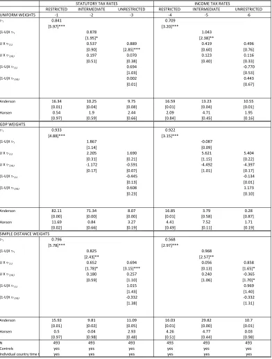
Table 5 replicates the regressions in columns 2, 4 and 6 of Tables 2 and 3 using uniform weights in the …rst panel, GDP weights in the second and, simple distance weights in the last one. The …rst three columns refer to statutory tax rates and the last three to income taxes. All the regressions are run using the full set of controls as in the previous tables as well as …xed e¤ects and individual time trends.
For statutory taxes we see that using uniform weights the coe¢cient estimates, and their signi…cance levels, do not di¤er much across the two tables. In our preferred speci…-cation, column 3, we see that (i) an EU country reacts to a one percentage point decrease in taxes in other EU countries by cutting its own taxes by the 0.88 points, while a non-EU country reacts by cutting 0.69 points, but the latter coe¢cient is not signi…cant. More-over a one percentage point cut undertaken by non-EU countries has the e¤ect of cutting 0.001 and 0.069 percentage points in non-EU and EU countries’ tax rates respectively; but both coe¢cients are again not signi…cant.
average of the EU members tax rates, since the largest European economies are also EU members. The results for this second exercise are reported in the second panel. The general picture is that this weighting scheme performs less well than e¤ective distance
or even uniform weights. Finally, if instead of e¤ective distance we use simple distance
weights, the coe¢cients of interest become unambiguously less signi…cant, showing that our e¤ective distance weights better explains corporate tax setting in western Europe. For income taxes instead, for all three sets of weights we do not …nd evidence of di¤erent behavior between and towards EU and non-EU countries, similarly to the results depicted in Table 3.
Finally, note that in our simple model union membership is treated as exogenous; we do believe that this the correct way to proceed given that EU formation is a very complex phenomenon which is driven by several forces, and it is a combination of both a political vision, based on European common history, as well as economic considerations. However in Table six we address a possible concern that current EU membership status
is endogenously determined along with taxes : this would cause the dummy as well as
£ and (1¡)£ to be endogenous. In the Table, we replicate columns …ve and
eight of Tables two and three, where the only di¤erence is that we instrument17 , £
and(1¡)£. The coe¢cient estimates in Table six are very similar both in magnitude
and in signi…cance compared with the corresponding coe¢cients in Tables two and three.
6. Conclusions
This paper has explored the impact of EU membership on …scal interactions among coun-tries. The starting point is the observation that the principal achievement of the European Union since its inception in 1957 has been the creation of a single market for goods, capi-tal and labour, and this should have contributed to lower the cost of investing abroad, i.e. by facilitating capital mobility. This might in turn have caused countries to react more to each others’ taxes.
We have developed a simple model of tax competition which veri…es this intuition. In the model, conditional on taxes, the size (in absolute terms) of cross-border investment between two countries is inversely proportional to the (marginal) cost of cross-border investment (these marginal costs could be physical, legal, or regulatory). EU membership is modelled as a reduction in ‘distance’ to other EU countries. We have derived precise
References
[1] Altshuler R., T. Goodspeed, (2006), "Follow the Leader? Evidence on European and U.S. Tax Competition", mimeo.
[2] Anselin, L. (1988), Spatial Econometrics: Methods and Models, Kluwer Academic
Publishers, Dordrecht.
[3] Anselin, L., Bera, K., Florax, R., Yoon, M. (1996), ”Simple diagnostic tests for spatial
dependence,” Regional Science and Urban Economics, 26, 77-104.
[4] Barrell, R., Pain, N. (1997), "The growth of foreign direct investment in Europe",
National Institute Economic Review, 160(1), 63-75.
[5] Barrell, R., Pain, N. (1998), "Real exchange rates, agglomerations and
irreversibil-ities: Macroeconomic policy and FDI in EMU", Oxford Review of Economic Policy
14 (3), 152-67.
[6] Barrell R., Pain N. (1999), "Domestic Institution, Agglomerations and Foreign Direct
Investment in Europe", European Economic Review, 43, 925-34.
[7] Besley T., R. Gri¢th, A. Klemm, (2001), "Empirical Evidence on Fiscal Interdepen-dence in OECD Countries ", mimeo.
[8] Blonigen, B. A., R. B. Davies, and K. Head (2003), "Estimating the
knowledge-capital model of the multinational enterprise: comment," American Economic
Re-view, 93, 980-94.
[9] Brenton P. (1996) “The Impact of the Single Market on Foreign Direct Investment
in the EU”, Report for DGII.
[10] Bretschger L., F. Hettich (2002), "Globalisation, capital mobility and tax
competi-tion: theory and evidence for OECD countries", European Journal of Political
Econ-omy, 18(4), 695-716.
[11] Brueckner, J. (1998), "Testing for strategic interaction among local governments: the
case of growth controls,” Journal of Urban Economics, 44, 438-67.
[12] Brueckner, J., Saavedra, L. (2001), "Do local governments engage in strategic
[13] Carr D. L., J. R. Markusen, and K. E. Maskus,(2001), "Estimating the
knowledge-capital model of the multinational enterprise," American Economic Review, 91,
693-708.
[14] Case, A., Hines, J., Rosen, H. (1993), ”Budget spillovers and …scal policy
interde-pendence,”Journal of Public Economics, 52, 285-307.
[15] Crabbe K., H. Vandenbussche (2008), "Are your …rm Taxes set in Warsaw? Spatial Tax Competition in Europe" LICOS Discussion Paper 216.
[16] Davies R., J. Voget (2009), "Tax Competition in an Expanding European Union", IIIS Discussion Paper 276.
[17] Devereux M. P., R. Gri¢th, A. Klemm, 2002. "Corporate income tax reforms and
international tax competition,"Economic Policy, 17(35), 449-95.
[18] Devereux, M. P, Lockwood, B., Redoano, M. (2007), "Horizontal and vertical Tax
Competition: Theory and Some Evidence from the USA", Journal of Public
Eco-nomics, 91, 451-79.
[19] Devereux, M. P, Lockwood, B., Redoano, M. (2008), "Do Countries Compete over
Corporate Tax Rates?", Journal of Public Economics, 92, 1210-35.
[20] Dreher A., (2006), "The in‡uence of globalization on taxes and social policy: An
empirical analysis for OECD countries", European Journal of Political Economy,
Volume 22, (1), 179-201.
[21] Egger,P., M. Pfa¤ermayr (2004), "Distance, trade and FDI: a Hausman-Taylor SUR
Approach" Journal of Applied Econometrics 19, 227-46.
[22] European Commission (2006), Final Report on "Study on FDI and regional devel-opment".
[23] Fuest, C. (2008), "The European Commission’s proposal for a common consolidated
corporate tax base", Oxford Review of Economic Policy, 24 (4), 720-39.
[24] Hau‡er, A., Klemm, A. Schjelderup G., (2008) "Redistributive taxation,
multina-tional enterprises, and economic integration," European Journal of Political
[25] K. Head and T. Mayer (2002), "Illusory Border E¤ects: Distance Mismeasurement In‡ates Estimates of Home Bias in Trade", CEPII Working Paper 2002-01.
[26] Kanbur, R., M. Keen (1993), "Jeux Sans Frontieres: Tax Competition and Tax
Coordination When Countries Di¤er in Size," American Economic Review, 83(4),
877-92.
[27] Kelejian, H, Prucha I.R. (1998), "A Generalized Spatial Two Stage Least Squares Procedure for Estimating a Spatial Autoregressive Model with Autoregressive
Dis-turbances", Journal of Real Estate Finance and Economics, 17, 297-312.
[28] Markusen, J. R., (2002), Multinational …rms and the theory of international trade,
MIT Press, Cambridge (Mass.).
[29] Mayer, T. and S. Zignago (2006): GeoDist: the CEPII’s distances and geographical database.
[30] Motta, M., and G.Norman (1996), "Does Economic Integration Cause FDI?"
Inter-national Economic Review 37, 757-73.
[31] Mendoza, E.G, Razin, A. and Tesar, L.L. (1994), “E¤ective tax rates in macroeco-nomics: cross country estimates of tax rates on factor incomes and consumption”,
Journal of Monetary Economics, 34, 297-323.
[32] Overesch M., J. Rincke (2008), "Tax Competition in Europe 1980-2007. Evidence from Dynamic Panel Data Estimation", mimeo.
[33] Persson T., G. Tabellini (2002), Political Economics: Explaining Economic Policy,
MIT Press.
[34] Petroulas, P. (2007), "The e¤ect of the Euro on foreign direct investment",European
Economic Review, 51(6), 1468-91.
[35] Redoano M. (2003), "Fiscal interaction among European countries", The Warwick Economics Research Paper Series (TWERPS), 680, University of Warwick, Depart-ment of Economics.
[37] Saavedra, L. (2001), "A model of welfare competition with evidence from AFDC",
Journal of Urban Economics, 47, 248-79.
[38] Schiavo S. (2007), "Common currencies and FDI ‡ows," Oxford Economic Papers,
59(3), 536-60.
[39] Solè-Ollè, A. (2003), "Electoral accountability and tax mimicking: the e¤ects of
electoral margins, coalition government and ideology, European Journal of Political
Economy, 19, 685-713.
[40] Van Aarle B. (1996), " The Impact of the Single Market Program on Trade and
Table 1(a): Country list and year of EU accession.
Year of Accession to the EU Countries
Original members Belgium, France, Germany, Italy, Luxemburg, the Netherlands. Joined in 1973 Denmark, Ireland, United Kingdom.
Joined in 1981 Greece.
Joined in 1986 Spain, Portugal.
Joined in 1995 Austria, Finland, Sweden. Never joined Switzerland, Norway
Table 1(b): Summary Statistics
Variable Source Observations Mean
Standard
Deviation Min Max
Statutory tax
rates Office of Tax PolicyReseach*
510 0.37 0.11 0.10 0.56
Income tax
rates Office of Tax PolicyReseach*
510 0.56 0.16 0.12 0.91
EU EU 510 0.63 0.48 0.00 1.00
R Our calculations 510 2.60 2.97 0.17 14.33
Election ComparativePolitical
Database***
510 0.28 0.45 0.00 1.00
GDPpc WDI** 510 2.17 0.92 0.50 5.30
PopDep WDI** 510 20.82 3.56 14.38 31.33
Population WDI** 510 21.75 24.12 0.34 82.09
PubExp WDI** 510 0.36 .084 0.13 0.55
* Available at otpr.org
** World Bank, World Development Indicators *** Available at nsd.uib.no
[image:32.595.75.507.112.212.2] [image:32.595.64.557.289.520.2]Graph 1. Statutory tax rates: trend by countries
Graph 2. Income tax rates: trend by countries
0
.2
.4
.6
0
.2
.4
.6
0
.2
.4
.6
0
.2
.4
.6
1970 1980 1990 2000 1970 1980 1990 2000 1970 1980 1990 2000
1970 1980 1990 2000 1970 1980 1990 2000
AUT BEL CHE DEU DNK
ESP FIN FRA GBR GRC
IRL ITA LUX NLD NOR
PRT SWE
Statutory Tax Rates
Geo-Distance Weighted Average Statutory Tax Rates EU-Geo-Distance Weighted Average Statutory Tax Rates Non-EU-Geo-Distance Weighted Average Statutory Tax Rates
year2
Graphs by code2
Statutory Tax Rates
0
.5
1
0
.5
1
0
.5
1
0
.5
1
1970 1980 1990 2000 1970 1980 1990 2000 1970 1980 1990 2000
1970 1980 1990 2000 1970 1980 1990 2000
AUT BEL CHE DEU DNK
ESP FIN FRA GBR GRC
IRL ITA LUX NLD NOR
PRT SWE
(Top) Income Tax Rates
Geo-Distance Weighted Average Income Tax Rates EU-Geo-Distance Weighted Average Income Tax Rates Non-EU-Geo-Distance Weighted Average Income Tax Rates
year2
Graphs by code2