A dynamic fake source algorithm for source location privacy in wireless sensor networks

(1)

http://wrap.warwick.ac.uk

Original citation:

Bradbury, Matthew S., Leeke, Matthew and Jhumka, Arshad (2015) A dynamic fake

source algorithm for source location privacy in wireless sensor networks. In: 2015 IEEE

Trustcom/BigDataSE/ISPA, Helsinki, 20-22 Aug 2015. Published in: 2015 IEEE

Trustcom/BigDataSE/ISPA, 1 pp. 531-538.

Permanent WRAP url:

http://wrap.warwick.ac.uk/75739

Copyright and reuse:

The Warwick Research Archive Portal (WRAP) makes this work by researchers of the

University of Warwick available open access under the following conditions. Copyright ©

and all moral rights to the version of the paper presented here belong to the individual

author(s) and/or other copyright owners. To the extent reasonable and practicable the

material made available in WRAP has been checked for eligibility before being made

available.

Copies of full items can be used for personal research or study, educational, or not-for

profit purposes without prior permission or charge. Provided that the authors, title and

full bibliographic details are credited, a hyperlink and/or URL is given for the original

metadata page and the content is not changed in any way.

Publisher’s statement:

“© 2015 IEEE. Personal use of this material is permitted. Permission from IEEE must be

obtained for all other uses, in any current or future media, including reprinting

/republishing this material for advertising or promotional purposes, creating new

collective works, for resale or redistribution to servers or lists, or reuse of any

copyrighted component of this work in other works.”

A note on versions:

The version presented here may differ from the published version or, version of record, if

you wish to cite this item you are advised to consult the publisher’s version. Please see

the ‘permanent WRAP url’ above for details on accessing the published version and note

that access may require a subscription.

(2)

A Dynamic Fake Source Algorithm for Source

Location Privacy in Wireless Sensor Networks

Matthew Bradbury, Matthew Leeke and Arshad Jhumka Department of Computer Science

University of Warwick, Coventry United Kingdom, CV4 7AL

{bradbury, matt, arshad}@dcs.warwick.ac.uk

Abstract—Wireless sensor networks (WSNs) are commonly used in asset monitoring applications, where it is often desirable for the location of the asset being monitored to be kept private. The source location privacy (SLP) problem involves protecting the location of a WSN source node from an attacker who is attempting to locate it. Among the most promising approaches to the SLP problem is the use of fake sources, with much existing research demonstrating their efficacy. Despite the effectiveness of the approach, the most effective algorithms providing SLP require network and situational knowledge that makes their deployment impractical in many contexts. In this paper, we develop a novel dynamic fake sources-based algorithm for SLP. We show that the algorithm provides state-of-the-art levels of location privacy under practical operational assumptions.

Keywords-Dynamic; Source Location Privacy; Sensor Networks;

I. INTRODUCTION

The ongoing development of wireless sensor network (WSN) technology has facilitated the development of many novel applications. One such application is asset monitoring, where a WSN is used to observe some properties of an impor-tant asset. Asset monitoring applications can range from safety-critical monitoring, including military and medical services [1], to non-critical monitoring, including temperature and humidity control [2]. Privacy, which can be described as the guarantee that information can only be observed or deciphered by those intended to observe or decipher it, is an important property in asset monitoring [3]. As WSNs operate in a broadcast medium, attackers can intercept messages and use the knowledge gained to attack the network or capture information on the asset.

Threats to privacy in asset monitoring applications can be classified along two dimensions: (i)content-basedthreats, and

(ii)context-basedthreats. Content-based privacy threats relate

to use of the content of the messages broadcast by sensor nodes. There has been much research in providing content privacy [4]. In contrast, context-based privacy threats relate to the context in which messages are broadcasts and how this can be observed by attackers. Context is a multi-attribute concept that encompasses situational aspects of broadcast messages, including environmental and temporal information. To address content-based privacy threats, nodes launching attacks are typically modelled as Byzantine nodes [5, 6], with cryptographic techniques often being used to address the threat itself [4, 5]. However, as cryptographic techniques can

not provide protection against context-based privacy threats, alternative approaches must be employed.

In asset monitoring applications the location of a source node, that is responsible for asset detection, often needs to be kept private. Typically a WSN will be deployed to monitor an asset, for example an endangered animal. When the nodes detect the presence of the asset, which we call the source

nodes, those source nodes will periodically send messages,

over a certain duration, to a dedicated node, called a sink, for data collection. If the location(s) of the source node(s) is compromised, either directly or inferred, then an attacker can capture the asset [3].

It is possible to infer message location information through various techniques, depending on the power of the attacker. For example, an attacker may have their own small wireless network, which we term anattacker network, that is capable of capturing messages at multiple locations [7]. On the other hand, an attacker may be a single entity with the same capabilities of a node in the network who uses the routing protocol to infer the source’s location [3]. Several possible techniques to handle the SLP problem have been proposed, with the technique often being influenced by the attacker model assumed [8, 9, 10, 11].

Previous fake source algorithms [12] have undertaken a search through many parameter values looking for performant settings under certain network configurations. Deploying the algorithm in a real-world scenario would require simulating the deployment to find good parameters. This is suboptimal, and as these parameters are fixed, it does not allow the SLP algorithm to respond to changing network conditions.

In this paper we present a novel dynamic algorithm to pro-vide SLP that requires no a priori network knowledge. This is achieved through the online estimation of the parameters identified as being significant in [12]. We perform extensive simulation to demonstrate that the dynamic algorithm pro-vides state-of-the-art levels of privacy, making it a viable option for WSN deployment in contexts where less in known about the operational environment.

(3)

II. RELATEDWORK

The SLP problem first appeared around 2005 in seminal work by Kamat et al. [3], shortly followed by the work of Ozturk et al. [13]. The authors of [3] proposed a formalisation of the SLP problem, and subsequently investigated several algorithms to enhance SLP. They proposed the fake source

technique, but indicated that it had poor performance despite being an expensive technique. It has since been shown that with certain attacker models, fake sources can provide SLP [14]. They went on to propose an algorithm calledphantom

routing, where messages are sent on a random walk of a given

length, followed by a normal flooding. The overall result im-plied that attackers can not fully trace messages back to a real source. Further energy-efficient random walk-based routing algorithms for WSNs have been developed [15, 16], though little is known as to whether these provide adequate SLP, with work demonstrating the efficacy of novel attacks on random walks [17]. Whilst investigating the global eavesdropper attacker model, [7] proposed every node broadcasting after τ seconds whether they had a packet to send or not. Recent work has also contributed the notion of condensation-based routing, which is a probabilistic broadcast algorithm [18].

The fake source technique, relies on a subset of network nodes acting as decoys for the real source by becoming fake sources. Fake sources will periodically broadcast fake messages that are indistinguishable from the normal messages sent by the (real) source, with the aim to convince an attacker that the fake source is actually the source node. When the set of nodes is the whole network, maximum SLP is achieved [7]. However, this configuration uses a large amount of energy, which reduces the network’s lifetime. Thus, an intelligent fake sources selection strategy is required. The fake source selection problem has been shown to be NP-complete, with a parameterised network-wide approach proposed to overcome the problem [12]. It was also shown that there is a trade-off to be made between SLP and energy used due to message retransmissions [19].

Combining fake sources and routing protocols, work in [20] and [21] contributed the notion of CEM and PEM respec-tively. CEM aims to trap the attacker in a cycle instead of letting them find the source node whereas PEM draws the attacker away using extended paths that broadcast fake messages. In [11] the authors proposed imposing a tree structure on the network using fake sources at the leafs with a focus on using the minimal energy possible at nodes one-hop from the sink node to lengthen the network’s lifetime.

There are several other research directions relating to the provision of privacy in WSNs. Some have investigated the problem of base station-location privacy [22] and providing location privacy to multiple nodes at once [23]. Others have focused on more powerful attackers, such as global attack-ers [7] or coordinated multiple attackattack-ers [14]. Whilst other research has focused on temporal privacy [24]. However, there is currently a lack of SLP-based techniques that provide SLP that obviates the need for network or application knowledge. We provide the first such technique in this paper.

III. ONLINEESTIMATION OFPARAMETERS

The efficiency of the static algorithm proposed in [12] depends on three parameters which capture the inherent trade-off between privacy and energy consumption. These parameters are: (i) the temporary fake source (TFS) duration (DT F S), (ii) the temporary fake source period (PT F S), and

(iii) the permanent fake source (PFS) period (PP F S). The

authors of [12] provided an exploration of the value space to understand their impact on SLP. However, these parameters must currently be fixed for all nodes on the basis of the deployer’s understanding of the operating environment and problem domain. Dynamically determining these parameters on a per node basis, obviating the need to incorporate operational knowledge, is the thrust of this paper.

In this section, we first provide a brief recap of the static SLP heuristic of [12] and derive the necessary equations for estimation of the identified parameters. The algorithm proposed in [12], henceforth referred to asstatic, is outlined below.

1) The source node sends a hnormali message Ni with

period Psrc, beginning withN1.

2) When the sink receivesN1it waits Psrc

2 then broadcasts

an hawayimessageAthat floods the network. 3) When a one-hop neighbour of the sink receives A it

becomes a TFS.

4) A TFS broadcasts a hfakei message Fi with period

PT F S for a duration of DT F S, before becoming a

normal node and broadcasting ahchooseimessageC. 5) When a normal node receives C it becomes a PFS if

the node believes itself to be the furthest node in the network from the sink, otherwise it will become a TFS. A PFS broadcasts a hfakei message Fi with period

PP F S.

• When a node receives a previously unencounteredNior AorFi it updates its last seen sequence number for that

message and rebroadcasts the message.

• When a node receives a previously unencountered C it updates its last seen sequence number for that message. The three parameters that were fixed in the static algorithm and need to be estimated in the dynamic algorithm are the TFS duration DT F S (derived in Subsection III-C), the TFS

periodPT F S (derived in Subsection III-D), and the PFS

pe-riodPP F S(derived in Subsection III-F). To aid in calculating

the TFS period, the number of fake messages to send on node j (#F(j)) is calculated (derived in Subsection III-E).

In order to derive these parameters certain pieces of in-formation about the network are required. This inin-formation comes in three categories, (i) parameters fixed at compile time of the firmware that are known by all nodes, (ii) information needed to derive the parameters but is not required during network execution and (iii) information that must be calcu-lated during network execution and passed to other nodes in the network.

The first piece of information required for implementation of the algorithm above, is the source period (Psrc), which

is fixed at compile time. This value is varied in the results presented in Section V.

(4)

The second piece of information is the time it takes for a message sent by one node to be received and processed by a neighbour (α). This delay has been the subject of research as it is an important value to take into account during clock synchronisation [25, 26]. In the context of this paper,αwill be small compared to the periods at which nodes will be broadcasting. This means that while it should be considered in intermediate calculations, it will ultimately be discounted in our final derivation.

Three pieces of network information are computed during execution: (i) the sink-source distance (∆ss), (ii) the sink

distance for noden (∆sink(n)) and (iii) the source distance

for noden(∆src(n)). All distances are calculated in hops.

For the following derivations we will look at the times certain events occur at.twill be used to indicate the current time.t= 0is the time at which the source node sends the first

hnormalimessage. Another piece of information that will be used in the derivation is the nodes that belong to the 1-hop neighbourhood ofj, this will be denoted 1HOPN(j).

A. Analogy

In tug-of-war, two teams are pulling on either end of a piece of rope, the team that pulls a marker on the rope over a certain point wins. When providing SLP we can think of sending messages as pulling on the rope, the source is on one side and the fake sources are on the other. The attacker is the marker that will cause one team to lose, i.e., when it captures the source because the pull from the source is greater than the pull from the fake sources. We will often refer to thepull

of the source or the fake sources during our explanations.

B. Message Timings

In order to derive appropriate expressions forDT F S,PT F S,

and PP F S, and hence develop the dynamic algorithm, the

timings associated with the reception of message can be con-sidered. Assuming there is no additional algorithm providing SLP, flooding is used to transmit messages, and that messages can take the shortest route between nodes; the following is true of the static algorithm behaviour:

• Theith _h_normal_i_{message is sent by the source at time:}

Ssrc(Ni) = (i−1)Psrc (1)

• An attacker will receive N1 at t = α∆ss and at this

time the attacker will have moved to be at (∆ss −1)

hops from the source. For theith hnormalimessage the attacker receives, the distance between the attacker and the source (∆as) will be:

∆as(Ni) =max(0,∆ss−i) (2)

• An attacker will receive theith_h_normal_i_{message at time:}

RA(Ni) =Ssrc(Ni) + ∆as(Ni−1)α (3)

When the dynamic algorithm is running the following infor-mation is known about the earliest timehawayimessages will be sent and received.

• ThehawayimessageAis sent by the sink at time:

Ssink(A) =Ssrc(N1) +α∆ss+

Psrc

2 (4)

• Node j will receiveAat the earliest at time:

Rj(A) =Ssink(A) +α∆sink(j) (5)

When node j receives an hawayi message A (and its hop count is 0), or it receives a hchoosei message the node becomes a TFS and starts broadcastinghfakeimessages. The time at which j becomes a TFS isτT F S(j), where:

τT F S(j) =    

  

Rj(A) if j∈1HOPN(sink)

τT F S(k) +

DT F S(k) +

α

if k ∈ 1HOPN(j)∧

∆sink(k)<∆sink(j)

(6)

The number of N messages sent between t = 0 and t = τT F S(j)isΣj(N):

Σj(N) = _τ

T F S(j)

Psrc

(7)

C. Calculating TFS Duration

1) Intuition: When a TFS is allocated, because it is by

nature temporary, it needs to have a finite duration during which it exerts a pull on the attacker greater than that of the source. The source period defines the pull that the source executes over the attacker, so the TFS needs to execute a pull greater than the source over this period. The source period is available to all nodes as a fixed constant, but to ensure that the network considers delays we need to instead defined the duration in terms of the time at which a node becomes a TFS (τT F S(j)) and how long the TFS has to broadcast

messages until the attacker receives the next normal message. This better captures the relationship than just using the source period.

2) Derivation: To calculate DT F S we set the duration to

be the difference in time between the TFS sending the first

hfakeimessage and the attacker receiving the next hnormali

message, less the time it takes to send the next hchoosei

message:

DT F S(j) =RA(NΣj(N)+1)−τT F S(j)−α (8)

For the case ∆sink(j) = 1, the attacker will have already

received N1 and the next hnormali message it will receive

isN2. The following timing information is known about the

nodes 1-hop away from the sink:

τT F S(j) =α∆ss+

Psrc

2 +α (9)

RA(N1) =α∆ss (10)

RA(N2) =Psrc+α(∆ss−1) (11)

Using this information the duration forj∈1HOPN(sink)is:

DT F S(j) =RA(N2)−τT F S(j)−α=

Psrc

2 −3α (12) The next step is to calculate the duration for nodes that are n-hops away from the sink, where n > 1. In this case the attacker has now received Nn and the duration of this TFS

is to last untilNn+1 is received. The knowledge about node

(5)

when the nodejthat isn-hops from the sink becomes a TFS atτT F S(j).

τT F S(j) =τT F S(k) +DT F S(k) +α

=τT F S(k) + (RA(Nn)−τT F S(k)−α) +α

=RA(Nn)

= (n−1)Psrc+α(∆ss−(n−1))

(13)

RA(Nn+1) =nPsrc+α(∆ss−n) (14)

Therefore the duration is given by:

DT F S(j) =RA(Nn+1)−τT F S(j)−α=Psrc−2α (15)

For nodes where∆sink(j) >1 the duration is equal to the

time that the attacker would receive the nexthnormali mes-sage, less the time it received the currenthnormalimessage andα.

DT F S(j) =RA(Ni+1)−RA(Ni)−α=Psrc−2α (16)

So for any nodej the DT F S(j)will be:

DT F S(j) = (_P

src

2 −3α if∆sink(j)∈ {1,⊥}

Psrc−2α otherwise

(17)

Asαis not available to the nodes during runtime,αis ignored in the final result.

DT F S(j) = (_P

src

2 if∆sink(j)∈ {1,⊥}

Psrc otherwise

(18)

To aid in handling imperfect passing of information around the network, when the node’s distance to the sink∆sink(j)is

unknown (i.e., set to⊥) the smaller duration should be used.

3) Code: The implementation of this follows from the

derivation. In the static algorithm where the fixed constant DT F Swas used, the functionDT F S(j)should now be called.

Algorithm 1Dynamic -DT F S: Modified actions when node

is Normal

1: receiveAway

seqNo,sinkD,ssd,maxHop,alg

→

. . .

2: ifawaySeqNo<seqNothen . . .

3: ifsinkD = 0then

−4: BECOMEFAKE(D←DT F S,P←PT F S,C ←hAwayi)

+4: BECOMEFAKE(D←DT F S(),P←PT F S,C ←hAwayi)

5: chooseSeqNo←chooseSeqNo + 1

. . .

6: receiveChoose

→

. . .

7: ifchooseSeqNo<seqNo∧SHOULDPROCESSCHOOSE(A)then 8: chooseSeqNo←seqNo

9: ifisPFSCandthen

10: BECOMEFAKE(D← ∞,P←DP F S,C ←hChoosei)

11: else

−12: BECOMEFAKE(D←DT F S,P←PT F S,C ←hChoosei)

+12: BECOMEFAKE(D←DT F S(),P←PT F S,C ←hChoosei)

Algorithm 2 Dynamic -DT F S:DT F S(j)

+1: functionDT F S( )

+2: if∆sink∈ {1,⊥}then returnPsrc₂

+3: else returnPsrc

D. Calculating TFS Period

1) Intuition: The TFS period defines how often messages

are sent, when combined with the TFS duration it can define or be defined in terms of the number ofhfakeimessages that will be sent over the duration. If a TFS was to sendn fake messages in this time period we might expect the attacker to be pulled back nhops. When considering collisions it is unlikely that the number of messages that reach the attacker from the right direction will be as high asn. Ideally the TFSs would send as many fake messages as would be needed to pull the attacker back from its actual position, but as we assume no node in the network can determine where the attacker is, the TFSs needs to pull back from a known distance elsewhere or estimate the attacker’s position.

A TFS must send at least 1 hfakei message to keep at parity with the number of hnormali messages sent. c > 1 messages need to be sent to ensure that at least one hfakei

message reaches the attacker when collisions occur. To pull an attacher backhhops,h×cdifferenthfakeimessages need to be sent.

2) Derivation: To establish PT F S we calculate the ratio

between the TFS durationDT F S(j)and the number ofhfakei

messages to send#F(j)(to be defined in Section III-E). Note

thatPT F Scan not allowed to go below3αas collisions would

then occur between the current and the previously broadcast

hfakeimessage.

PT F S(j) =max(3α,

DT F S(j)

#F(j)

) (19)

Again asαis unavailablePT F S(j)is finally defined without

it. A caveat is that this requires#F(j)to be defined in such

a way that it does not lead to PT F S(j) being set to 3α or

less.

PT F S(j) =

DT F S(j)

#F(j)

(20)

3) Code: When a node becomes a TFS, instead of

ini-tialising the TFS period to the fixed constant used in the static algorithmPT F S the function PT F S(j)should be used

instead.

Algorithm 3Dynamic -PT F S: Modified actions when node

is Normal

1: receiveAway

→

. . .

2: ifawaySeqNo<seqNothen . . .

3: ifsinkD = 0then

−4: BECOMEFAKE(D←DT F S(),P←PT F S,C ←hAwayi)

+4: BECOMEFAKE(D←DT F S(),P←PT F S(),C ←hAwayi)

5: chooseSeqNo←chooseSeqNo + 1

. . .

6: receiveChoose

→

. . .

9: ifisPFSCandthen

10: BECOMEFAKE(D← ∞,P←DP F S,C ←hChoosei)

11: else

−12: BECOMEFAKE(D←DT F S(),P←PT F S,C ←hChoosei)

+12: BECOMEFAKE(D ← DT F S(), P ← PT F S(),

C ←hChoosei)

(6)

Algorithm 4 Dynamic -PT F S:PT F S(j)

+1: functionPT F S( )

+2: returnDT F S()÷#F()

E. Calculating Number of Fake Messages to Send

1) Derivation: The final setting for TFSs is number of

messages a TFS needs to send. Two approaches are provided to calculate this setting.

a) Pull From Attacker:

#F(j) =max⊥(1,2∆sink(j)) (21)

This approach aims to pull the attacker back from its esti-mated position assuming no SLP protection. In this case we assume that TFS nodes propagate away from the source at the same rate that an attacker moves towards the source. This can be a reasonable assumption when the duration of the TFS is equal to the source period. This means that a TFS will need to send twice the∆sink(j)to dissuade the attacker back from

its position.∆sink(j)message are needed to pull back from

the sink to the TFS, another∆sink(j) messages are needed

to pull the attacker from its position back to the sink.

b) Pull From Sink:

#F(j) =max⊥(1,

 



∆sink(j) if ∆src(j) = ⊥ ∨

∆ss=⊥

∆src(j)−∆ss otherwise

)

(22) This approach aims is to pull the attacker back from the sink’s location. This approach is less aggressive compared to the previous approach and isn’t as focused on trying to pull the attacker all the way back, but instead keeping it in a location between the TFS and the source. An important benefit of this approach is that∆src(j)−∆ss is used to calculate the

sink distance. This means that a TFS closer to the source will send fewer messages than TFS further away. Leading to better message sending patterns that should prefer leading the attacker away from the source. We explore this further in Section V, where the implications for privacy and energy consumption are considered for each approach.

2) Code: Two#F(j)algorithms are presented here, only

one is chosen to be active at compile time.

Algorithm 5 Dynamic -#F:#F(j)- Pull From Attacker

+1: function#F( )

+2: returnmax⊥(1,2∆sink)

Algorithm 6 Dynamic -#F:#F(j)- Pull From Sink

+1: function#F( )

+2: if∆src=⊥ ∨∆ss=⊥then returnmax⊥(1,∆sink)

+3: else returnmax⊥(1,∆src−∆ss)

Algorithm 7Dynamic -#F: Modified Receivehchooseiby

Normal nodes

1: receiveChoose

→ +2: ∆sink←min⊥(∆sink,sinkD + 1)

3: . . .

F. Calculating PFS Period

1) Intuition: Unlike when calculating the TFS period,

the PFS is ∞ meaning reasoning about a fixed number of messages to be sent in a given time period isn’t possible. So determining the PFS period needs a different approach.

By the time that a PFS has been created, many TFSs should have been involved with pulling the attacker away from the source. This means that the PFS shouldn’t need to send as manyhfakei messages as a TFS. It will still need to send at least 1hfakeimessage for eachhnormalimessage sent by the source, plus some extra to consider collisions.

2) Derivation: If an attacker can be guaranteed to have

been moved far enough from the source by TFSs then having PP F S(j) =Psrcwould be preferable. However, the attacker’s

position should not be relied upon to be far enough away, meaning the algorithm requires PP F S(j)< Psrc, such that

any PFSs retains the ability to pull back the attacker and cope with collisions ofhfakeimessages.

A lower bound on the periodPP F S(j)≥αexists, as the

PFS cannot physically send messages more often than that. There will also exist an upper bound of PP F S(j)< Psrc as

the PFS should not broadcast slower than the source. The technique used here is to set the PFS period to the source period based multiplied the receive ratio of hfakei

messages at the source (ψsrc(F)). This is justified because it

means for everyhnormalimessage sent the PFS should send enough hfakei messages for the attacker to receive at least onehfakeimessage.

PP F S(j) =max(Psrc×ψsrc(F),3α) (23)

In order to calculate this receive ratio, the source node needs to keep a record of the number ofhfakei messages sent and received. It can do this by using the sequence counter as the number sent and then record the number of times that counter was updated as the number received. This information must be transmitted back to the PFS, where it is needed, using hnormali messages. This is best effort as a PFS may not receive everyhnormalimessage sent.

ψsrc(F) =

fake messages received + 1

fake sequence number + 1 (24)

Removing theαterms this gives:

PP F S(j) =Psrc×ψsrc(F) (25)

3) Code: The code for this implementation requires

gath-ering extra knowledge about srcFakeIncs and srcFakeNo and passing it to other nodes in the network usinghnormali

messages.

Algorithm 8 Dynamic -PP F S:PP F S(j)andψsrc(F)

+1: functionPP F S( )

+2: returnPsrc×ψsrc(F)

+3: functionψsrc(F)

(7)

Algorithm 9Dynamic -PP F S: Modified actions when node

is Normal

1: receiveChoose

→

. . .

4: ifisPFSCandthen

−5: BECOMEFAKE(D← ∞,P←PP F S,C ←hChoosei)

+5: BECOMEFAKE(D← ∞,P←PP F S(),C ←hChoosei)

6: else

7: BECOMEFAKE(D←DT F S(),P←PT F S(),C ←hChoosei)

Algorithm 10Dynamic -PP F S: Modified Source Actions

1: receiveFake

seqNo,. . .

→

2: iffakeSeqNo<seqNothen

+3: srcFakeIncs←srcFakeIncs + 1

4: . . .

5: timeout(normalTimer)→

6: normalSeqNo←normalSeqNo + 1

−7: BCASTNormal

normalSeqNo,0,j,firstSrcD,∆ss

+7: BCASTNormal

normalSeqNo,0,j,firstSrcD,

∆ss,fakeSeqNo,srcFakeIncs

8: normalTimer←Psrc

Algorithm 11Dynamic -PP F S: Modified Receivehnormali

1: receiveNormal

seqNo,srcD,srcID,maxHop,

ssd,fakeNo,fakeIncs

→ +2: srcFakeNo←MAX(srcFakeNo,fakeNo)

+3: srcFakeIncs←MAX(srcFakeIncs,fakeIncs) 4: . . .

5: ifnormalSeqNo<seqNothen

6: . . .

−7: BCASTNormal

seqNo,srcD + 1,srcID,

MAX(firstSrcD,maxHop),∆ss

+7: BCASTNormal

*_seqNo_,_{srcD + 1}_,_srcID_,

MAX(firstSrcD,maxHop),∆ss,

srcFakeNo,srcFakeIncs

+

G. Additional Dynamic Algorithm Implementation

One final change was included and that was to increase the area around the source node in whichhchooseimessages are ignored. By ignoring hchoosei messages in this area, fake sources will not be allocated in the direction of the source.

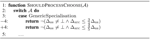
Algorithm 12Dynamic: Modified ShouldProcessChoose

1: functionSHOULDPROCESSCHOOSE(A)

2: switchAdo

3: caseGenericSpecialisation

−4: return¬(∆ss6=⊥ ∧∆src≤ 3₄∆ss)

+4: return¬(∆ss6=⊥ ∧∆src≤ 4₅∆ss)

5: . . .

IV. EXPERIMENTALSETUP

In this section we describe the simulation environment and protocol configurations that were used to generate the results presented in Section V.

A. Simulation Environment and Network Configuration

The TOSSIM (V2.1.2) simulation environment was was used in all experiments [27]. TOSSIM is a discrete event simulator

capable of accurately modelling sensor nodes and the modes of communications between them.

[image:7.612.52.301.559.625.2]

A square grid network layout of size n×n was used in all experiments, where n ∈ {11,15,21,25}, i.e., networks with 121, 225, 441 and 625 nodes respectively. The node neighbourhoods were generating using LinkLayerModel with the parameters shown in table I. Noise models were created using the first 1000 lines ofmeyer-heavy.txt1. A single source node generated messages and a single sink node collected messages. The source and sink nodes were distinct and assigned positions in the SourceCorner configuration from [12]. The rate at which messages from the real source were generated was varied, as shown in Section V. Exactly 500 repeats were performed for each source location, and for each combination of parameters. Nodes were located 4.5 meters apart. The node separation distance was determined experimentally, based on observing the pattern of transmis-sions in the simulator. This separation distance ensured that messages (i) pass through multiple nodes from source to sink, (ii) can move only one hop at a time, and (iii) will usually only be passed to horizontally or vertically adjacent nodes.

TABLE I: LinkLayerModel Parameters

Name Value

PATH LOSS EXPONENT 4.7

SHADOWING STANDARD DEVIATION 3.2

D0 1.0

PL D0 55.4

NOISE FLOOR −105

S [0.9−0.7;−0.7 1.2]

WHITE GAUSSIAN NOISE 4

B. Attacker Model

A reactive attacker model based on the patient adversary introduced in [3] is used. The attacker initially starts at the sink. When a message is received the attacker will move to the 1-hop source’s location if that message has not been received before. To detect if a message has been received before, we assume that an attacker has access to the message type and sequence number. Once the source has been found the attacker will no longer move. This is commensurate with the attack models used in [12], [19] and [14].

C. Safety Period

A metric called safety period was introduced in [3] to capture the number of messages needed to capture the source. The higher the safety period is, the higher is the privacy level. The problem with this metric is that simulation time may be extremely large. We thus use an alternative, but analogous, definition for safety period: for each network size and source rate, using flooding, we calculate the average time it takes to detect the real source (i.e., capture the asset). Since this value is for normal flooding network, we use a larger value of safety period to allow the attacker the chance of rectifying a move in the wrong direction. The safety period, for each network size and rate, for flooding is shown in table II. The safety period value used is double the average time taken for source detection.

1_{meyer-heavy.txt is a noise sample file provided with TOSSIM.}

(8)

[image:8.612.315.565.60.240.2]

TABLE II: Safety period for each network size and send rate.

Network Size Safety Period (seconds)

1/sec 2/sec 4/sec 8/sec

11×11 47.30 25.16 13.35 7.51

15×15 72.30 36.54 18.50 10.05

21×21 103.76 53.59 27.58 14.01

25×25 126.14 63.21 33.19 17.06

D. Simulation Experiments

An experiment constituted a single execution of the simu-lation environment using a specified protocol configuration, network size and safety period. An experiment terminated when the source node had been captured by an attacker or the safety period had expired. An attacker was implemented based on the log output from TOSSIM. It maintains internal state about its location using node identifiers. When a node re-ceives a message, if the attacker is at that location it will move based on the attacker model specified in Subsection IV-B.

V. RESULTS

In this section we describe the results of the dynamic al-gorithm via a comparison between them and the static SLP algorithm.

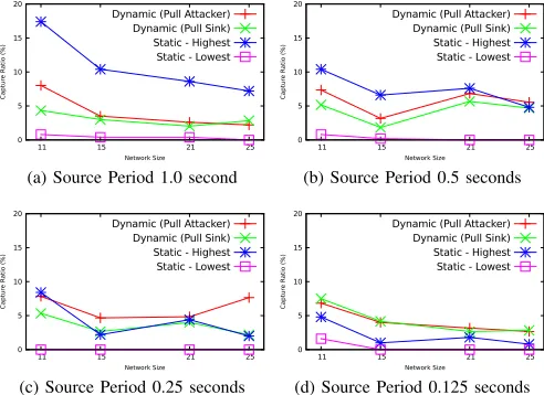
From our simulations we collected various metrics about the performance of the static and dynamic algorithms. Two of those metrics are included in the results graphs: i) capture ratio and ii) average number of fake messages sent. Capture ratio is defined as the number of simulations in which the source was captured by the attacker within the safety period (see Subsection IV-C). Capture ratio is a metric that can be used to analyse how well the algorithm provides SLP. The second metric, average number of fake messages sent is the average of the total number of fake messages sent by all nodes in each simulation. This metric is useful in providing the amount of energy that the SLP algorithms use to produce fake messages to pull the attacker away.

0 5 10 15 20

11 15 21 25

Captur

e R

atio (%)

Network Size

Dynamic (Pull Attacker) Dynamic (Pull Sink) Static - Highest Static - Lowest

(a) Source Period 1.0 second 0 5 10 15 20

11 15 21 25

Captur

e R

atio (%)

Network Size

(b) Source Period 0.5 seconds

0 5 10 15 20

11 15 21 25

Captur

e R

atio (%)

Network Size

(c) Source Period 0.25 seconds 0 5 10 15 20

11 15 21 25

Captur

e R

atio (%)

Network Size

[image:8.612.84.269.76.133.2]

(d) Source Period 0.125 seconds

Fig. 1: The capture ratio for two dynamic#F(j)

approaches and the minimum and maximum static results. In terms of the dynamic algorithm’s ability to provide SLP, we see that the capture ratio results tend to lie between

0 100000 200000 300000 400000 500000 600000

11 15 21 25

Fak

e Messages Sent

Network Size

(a) Source Period 1.0 second

0 100000 200000 300000 400000 500000 600000

11 15 21 25

Fak

e Messages Sent

Network Size

(b) Source Period 0.5 seconds

0 100000 200000 300000 400000 500000 600000

11 15 21 25

Fak

e Messages Sent

Network Size

(c) Source Period 0.25 seconds

0 100000 200000 300000 400000 500000 600000

11 15 21 25

Fak

e Messages Sent

Network Size

(d) Source Period 0.125 seconds

Fig. 2: The average number of fake messages sent for two dynamic #F(j)approaches and the minimum and

maximum static results.

the best and worst static results for the two slower source periods 1.0 and 0.5 seconds. For the periods of 0.25 and 0.125 seconds the capture ratios tend to be similar or worse than the worst case static results. It would appear that the dynamic algorithm performs better for longer source periods than slower.

There are a couple of plausible causes of this behaviour. It could be that the fake message rates are too high for these shorter periods, leading to a greater number of collisions and a reduction in the pull the fake sources have over the attacker. However, we believe the most likely one is that, at those very low periods, the message processing delay at each node has higher significance. However, we assumed no processing delay at the nodes. Specifically, at such low periods, the delay in processing messages is non-negligible with respect to the source period.

In most cases the Pull Attacker approach shows a greater energy usage and a greater capture ratio than the

[image:8.612.56.302.506.685.2]

(9)

VI. DISCUSSION

A. Assumptions on the Magnitude ofα

The time between one node sending a message and another node receiving a message (denotedα) has been assumed to be a small value. During simulationsαwas observed to be about 6ms. In our derivation of the dynamic parameters we made the assumption thatαwould have a negligible impact when it turned up in the penultimate derivation of the parameters, that allowed it to be removed from the final derivation. Doing so opens the fake sources to potentially become out-of-sync with the normal source. Ifαis small then it is unlikely that this will have a large impact as collisions are likely to be a bigger factor. Ifαis large with respect to the source period, then the fake sources could become out-of-sync quickly and often. We predict that this could lead to poor performance, meaning that in this case the extra effort to estimate and use αmay be necessary. Although we would be surprised to find WSN radio transmissions of hundreds of bytes lasting in the region of seconds.

B. TFS Duration

In this work the TFS duration is calculated based on the time between a node becoming a TFS and an attacker receiving the nexthnormalimessage. Previously it has been observed that longer TFS durations tended to produce lower capture ratios [12]. Changing the TFS duration to pull back over more than onehnormalimessage may improve the privacy provided.

VII. CONCLUSION

In this paper, we have developed a novel SLP algorithm that performs online estimation of parameters, making it attractive for deployment. We have derived the conditions required for estimating parameters that are paramount for the efficiency of the SLP protocol. We have shown that, in general, the results obtained by the dynamic algorithm are comparable to state-of-the-art results when performing a traversal of the value space of the important parameters.

REFERENCES

[1] A. Milenkovi´c, C. Otto, and E. Jovanov, “Wireless sensor networks for personal health monitoring: Issues and an implementation,”Computer Communications, vol. 29, no. 1314, pp. 2521 – 2533, 2006, wirelsess Senson Networks and Wired/Wireless Internet Communications. [2] A. Mainwaring, D. Culler, J. Polastre, R. Szewczyk, and J. Anderson,

“Wireless sensor networks for habitat monitoring,” inProceedings of the 1st ACM International Workshop on Wireless Sensor Networks and Applications, ser. WSNA ’02. ACM, 2002, pp. 88–97.

[3] P. Kamat, Y. Zhang, W. Trappe, and C. Ozturk, “Enhancing source-location privacy in sensor network routing,” in25thIEEE International Conference on Distributed Computing Systems, 2005. ICDCS 2005. Proceedings., June 2005, pp. 599–608.

[4] A. Perrig, J. Stankovic, and D. Wagner, “Security in wireless sensor

networks,”Communications of the ACM - Special Issue on Wireless

Sensor Networks, vol. 47, no. 6, pp. 53–57, June 2004.

[5] L. Lamport, R. Shostak, and M. Pease, “The byzantine generals

problem,”ACM Transactions on Programming Languages and Systems,

vol. 4, no. 3, pp. 382–401, July 1982.

[6] M. Nesterenko and S. Tixeuil, “Discovering network topology in the

presence of byzantine faults,” IEEE Transactions on Parallel and

Distributed Systems, vol. 20, no. 12, pp. 1777–1789, December 2009. [7] K. Mehta, D. Liu, and M. Wright, “Location privacy in sensor networks

against a global eavesdropper,” in Proceedings of the 15th IEEE

International Conference on Network Protocols, October 2007, pp. 314–323.

[8] S. Armenia, G. Morabito, and S. Palazzo, “Analysis of location privacy/energy efficiency tradeoffs in wireless sensor networks,” in

Proceedings of the 6th International IFIP-TC6 Networking Conference on Ad Hoc and Sensor Networks, Wireless Networks, Next Generation Internet, November 2007, pp. 215–226.

[9] S.-W. Lee, Y.-H. Park, J.-H. Son, S.-W. Seo, U. Kang, H.-K. Moon, and M.-S. Lee, “Source-location privacy in wireless sensor networks,”

Korea Institute of Information Security and Cryptology Journal, vol. 17, no. 2, pp. 125–137, April 2007.

[10] J. Yao and G. Wen, “Preserving source-location privacy in energy-constrained wireless sensor networks,” inProceedings of the 28th In-ternational Conference on Distributed Computing Systems Workshops, June 2008, pp. 412–416.

[11] J. Long, M. Dong, K. Ota, and A. Liu, “Achieving source location privacy and network lifetime maximization through tree-based diver-sionary routing in wireless sensor networks,”Access, IEEE, vol. 2, pp. 633–651, 2014.

[12] A. Jhumka, M. Bradbury, and M. Leeke, “Fake source-based source location privacy in wireless sensor networks,”Concurrency and Com-putation: Practice and Experience, April 2014.

[13] C. Ozturk, Y. Zhang, and W. Trappe, “Source-location privacy in energy-constrained sensor network routing,” inProceedings of the 2nd ACM workshop on Security of ad hoc and sensor networks, ser. SASN

’04. New York, NY, USA: ACM, 2004, pp. 88–93.

[14] A. Jhumka, M. Leeke, and S. Shrestha, “On the use of fake sources for source location privacy: Trade-offs between energy and privacy,”The Computer Journal, vol. 54, no. 6, pp. 860–874, June 2011.

[15] H. Tian, H. Shen, and T. Matsuzawa, “Random walk routing in wsns with regular topologies,”Journal of Computer Science and Technology, vol. 21, no. 4, pp. 496–502, 2006.

[16] I. Mabrouki, X. Lagrange, and G. Froc, “Random walk based routing

protocol for wireless sensor networks,” in Proceedings of the 2nd

international conference on Performance Evaluation Methodologies and Tools, 2007.

[17] R. Shi, M. Goswami, J. Gao, and X. Gu, “Is random walk truly memoryless — traffic analysis and source location privacy under

random walks,” in INFOCOM, 2013 Proceedings IEEE, April 2013,

pp. 3021–3029.

[18] F. Palmieri and A. Castiglione, “Condensation-based routing in mobile ad-hoc networks,”Mob. Inf. Syst., vol. 8, no. 3, pp. 199–211, Jul. 2012. [19] A. Thomason, M. Leeke, M. Bradbury, and A. Jhumka, “Evaluating the impact of broadcast rates and collisions on fake source protocols for source location privacy,” in2013 12th IEEE International Conference on Trust, Security and Privacy in Computing and Communications (TrustCom), July 2013, pp. 667–674.

[20] Y. Ouyang, Z. Le, D. Liu, J. Ford, and F. Makedon, “Source location privacy against laptop-class attacks in sensor networks,” in Proceed-ings of the 4th International Conference on Security and Privacy in Communication Networks, September 2008, pp. 22–25.

[21] W. Tan, K. Xu, and D. Wang, “An anti-tracking source-location privacy protection protocol in wsns based on path extension,”Internet of Things Journal, IEEE, vol. 1, no. 5, pp. 461–471, Oct 2014.

[22] J. Deng, R. Han, and S. Mishra, “Countermeasures against traffic analysis attacks in wireless sensor networks,” in Proceedings of the 1st International Conference on Security and Privacy for Emerging Areas in Communications Networks, 2005, pp. 113–126.

[23] H. Chen and W. Lou, “From nowhere to somewhere: Protecting end-to-end location privacy in wireless sensor networks,” inPerformance Computing and Communications Conference (IPCCC), 2010 IEEE 29th International, Dec 2010, pp. 1–8.

[24] P. Kamat, W. Xu, W. Trappe, and Y. Zhang, “Temporal privacy in wireless sensor networks: Theory and practice,”ACM Transactions on Sensor Networks, vol. 5, no. 4, p. 24 (Article 28), November 2009. [25] K. Liu, Q. Ma, H. Liu, Z. Cao, and Y. Liu, “End-to-end delay

measurement in wireless sensor networks without synchronization,” in Mobile Ad-Hoc and Sensor Systems (MASS), 2013 IEEE 10th International Conference on, Oct 2013, pp. 583–591.

[26] Y.-C. Wu, Q. Chaudhari, and E. Serpedin, “Clock synchronization of wireless sensor networks,”Signal Processing Magazine, IEEE, vol. 28, no. 1, pp. 124–138, Jan 2011.

[27] P. Levis, N. Lee, M. Welsh, and D. Culler, “Tossim: Accurate and scalable simulation of entire tinyos applications,” inProceedings of the 1st International Conference on Embedded Networked Sensor Systems,

ser. SenSys ’03. New York, NY, USA: ACM, 2003, pp. 126–137.