http://go.warwick.ac.uk/lib-publications
Original citation:
Griffin, J. E., Kolossiatis, M. and Steel, Mark F. J.. (2013) Comparing distributions by
using dependent normalized random-measure mixtures. Journal of the Royal Statistical
Society : Series B (Statistical Methodology)
Permanent WRAP url:
http://wrap.warwick.ac.uk/53118
Copyright and reuse:
The Warwick Research Archive Portal (WRAP) makes the work of researchers of the
University of Warwick available open access under the following conditions. Copyright ©
and all moral rights to the version of the paper presented here belong to the individual
author(s) and/or other copyright owners. To the extent reasonable and practicable the
material made available in WRAP has been checked for eligibility before being made
available.
Copies of full items can be used for personal research or study, educational, or
not-for-profit purposes without prior permission or charge. Provided that the authors, title and
full bibliographic details are credited, a hyperlink and/or URL is given for the original
metadata page and the content is not changed in any way.
Publisher’s statement:
http://dx.doi.org/10.1111/rssb.12002
A note on versions:
The version presented in WRAP is the published version or, version of record, and may
be cited as it appears here.
©2013 Royal Statistical Society 1369–7412/13/75000
75,Part3,pp.
Comparing distributions by using dependent
normalized random-measure mixtures
J. E. Griffin,
University of Kent, Canterbury, UK
M. Kolossiatis
Cyprus University of Technology, Limassol, Cyprus
and M. F. J. Steel
University of Warwick, Coventry, UK
[Received December 2010. Final revision September 2012]
Summary.A methodology for the simultaneous Bayesian non-parametric modelling of several distributions is developed. Our approach uses normalized random measures with independent increments and builds dependence through the superposition of shared processes. The prop-erties of the prior are described and the modelling possibilities of this framework are explored in detail. Efficient slice sampling methods are developed for inference.Various posterior summaries are introduced which allow better understanding of the differences between distributions. The methods are illustrated on simulated data and examples from survival analysis and stochastic frontier analysis.
Keywords: Bayesian non-parametrics; Dependent distributions; Dirichlet process; Normalized generalized gamma process; Slice sampling; Utility function
1. Introduction
This paper considers the non-parametric modelling of data divided into different groups and the comparison of their distributions. For example, we may observe the results of different medical treatments or the performance of firms with different management structures. Statistical analysis will often concentrate on inference about the differences in the distributions. Analysis of variance (ANOVA) focuses on differences between means for different groups and links these to the effects of each factor. However, differences between groups may not be well modelled by restricting attention to location. For example, if there are distinct subpopulations within the observations then each group may contain different proportions of each subpopulation and a full summary of the differences would involve identifying parts of the support on which the two distributions place substantially different masses. We implement a fully Bayesian analysis by firstly placing a prior on the distributions and secondly defining a decision analysis which reports where the distributions are similar or substantially different.
Address for correspondence: M. F. J. Steel, Department of Statistics, University of Warwick, Coventry, CV4 7AL, UK.
E-mail: [email protected]
We use a Bayesian non-parametric mixture model approach to understand the differences between the distributions. LetF1,F2,: : :,Fqbe the (continuous) distributions of the observations
forqdifferent groups; then an infinite mixture model assumes that the density for thegth group
is
fg=
k.·|θ/dGg.θ/
wherek.·|θ/is a density parameterized byθandGg is a discrete random-probability measure.
Since the measure is discrete, it can be represented as
Gg=
∞
i=1
wg,iδθg,i
whereδxis the Dirac delta function that places mass 1 atxandθg,1,θg,2, . . . andwg,1,wg,2, . . . are infinite sequences of random variables for whichΣ∞i=1wg,i=1 andwg,i>0 for allgandi. It
follows that the mixture model for groupgcan be written as
fg=
∞
i=1
wg,ik.·|θg,i/ .1/
or, alternatively, the model can be represented hierarchically for an observationyg,jdrawn from
Fgas follows:
yg,j∼k.·|θg,sg,j/, p.sg,j=i/=wg,i
wheresg,j is an allocation variable indicating to which component distributionk.·|θ/thejth
observation in groupgis allocated. The groups will often be formed by all possible combinations
of some categorical covariates and we shall denote those covariates byzgfor thegth group. This
is a very general model which encompasses many previously proposed models. The ANOVA
dependent Dirichlet process model of De Iorioet al.(2004) assumes thatwg,i=wiand the density
kis a normal distribution with meanzTgβi, whereβiis a vector of parameters, and varianceσ2.
This allows the means of the different components to change with covariates.
A popular approach allows the weights to depend on covariates and setsθg,i=θi so that
the location of the components is fixed across each group. A finite mixture of normals model
along these lines was proposed by Rodriguezet al.(2009) who allowed the component weights
to depend on covariates. Alternatively, the weights can be modelled through combinations of random variables, which encourages correlation between the random distributions. The matrix
stick breaking process of Dunson et al. (2008) focuses on groups which are formed by the
combination of two factors, sayzg,1andzg,2, each with a finite number of levels. They defined
the weights by using the stick breaking construction
wg,i=Vzg, 1,iUzg, 2,i
l<i
.1−Vzg, 1,lUzg, 2,l/
where Uj,i andVj,i are independent, beta-distributed random variables. M ¨ulleret al. (2004)
assumed that
fg=ψ
∞
i=1
wgÅ,ik.·|θÅg,i/+.1−ψ/∞
i=1
wik.·|θi/
where 0ψ1. The distribution of thegth group is a mixture of a common component shared
by all groups and an idiosyncratic component. The parameterψis the weight that is placed on
the idiosyncratic component and so affects the correlation between distributions.
Gg|G0 IID
∼DP.MG0/, g=1,: : :,q, G0∼DP.M0H/, .2/
where DP.MH/indicates a Dirichlet process with mass parameterM >0 and centring (or base)
distributionH. The distributions are exchangeable and this structure allows clusters to be shared
by different groups (owing to the discrete nature of the Dirichlet process at both levels). If the hierarchical Dirichlet process is used as the mixture distribution in the mixture models then we
have something of the form of model (1). Tehet al.(2006) derived the stick breaking construction
forwg,1,wg,2,wg,3, . . .. The model can be extended to more levels of hierarchy in the standard way. This model assumes that distributions are exchangeable at some level. In contrast, the present paper will mostly concentrate on the problem where groups are defined by covariates. There is normally no natural nesting in these settings, so hierarchical models will then not be appropriate. Note also that we shall focus on categorical covariates, which naturally lead to a finite number of groups.
We propose to use a normalized superposition of random measures to induce dependence. This general framework leads to dependence structures that can be fairly easily controlled through the mass parameters of the underlying component measures and extends naturally to any number of groups. In fact, we can use this framework to model separately the mass shared by any subset of the groups or we can use simpler settings, depending on the flexibility of the dependence structure that we want to assume. We can formally conduct model selection by using point mass priors on the mass parameters corresponding to the components. Alternatively, we use shrinkage priors for the mass parameters to ensure consistent priors across different levels of model complexity. For posterior inference, we propose slice sampling Markov chain Monte Carlo (MCMC) methods, used in combination with a split–merge move. We also introduce ways of summarizing the differences between the non-parametric distributions for each group, based on decision theoretic ideas.
The paper is organized as follows. Section 2 describes the construction of random proba-bility measures by normalization and our proposed framework for modelling dependence by using normalized random measures, Section 3 describes efficient MCMC sampling methods for inference, Section 4 discusses a decision theoretic approach to comparing distributions, Section 5 analyses simulated data and presents real data applications to survival analysis and stochastic frontier modelling, whereas Section 6 concludes.
2. Introducing dependence in normalized random measures
2.1. General framework
Normalized random measures with independent increments (known in the literature as
‘NRMIs’) are a class of non-parametric priors for a random probability measureGconstructed
by normalizing a positive random measure G˜ with independent increments and support Ω
(usually, a subset ofRm). Thus, for any measurable setB∈Ωwe define
G.B/= ˜G.B/=G.˜ Ω/:
Throughout the paper we shall useGto represent the normalized version of a random measure
˜
G. Generally, we shall concentrate on random measures which only contain jumps and write
˜ G=∞
i=1
Jiδθi,
almost surely which happens ifζ.x/dxis infinite. The NRMI can be employed as the prior
of the mixing measureGin an infinite mixture modelf.y/=k.y|θ/dG.θ/to define an NRMI
mixture. This class of processes and their use in mixture models was studied in general by James
et al.(2009). We focus on homogeneous NRMIs, which impliesa prioriindependence between
the jumps and the locations. Jameset al. (2009) showed that these processes can be defined
on arbitrary spaces. Several previously proposed processes fall within this class. The Dirichlet
process (Ferguson, 1973) occurs ifG˜ is a gamma process, for which
ζ.x/=Mx−1exp.−x/, M >0:
This can be generalized to the normalized generalized gamma (NGG) process (Lijoiet al., 2007)
which is constructed by normalizing a generalized gamma process (Brix, 1999) for which
ζ.x/= M Γ.1−a/x
−1−aexp.−λx/, M >0, 0< a <1, λ0: .3/
This process tends to the Dirichlet process asa→0 andλ=1. The normalized inverse Gaussian
process (Lijoiet al., 2005) occurs ifa=0:5 andλ=1. Another special case is the normalized
stable process of Kingman (1975), which corresponds toλ=0.
Dependence between two distributionsG1andG2is introduced through the unnormalized
random measuresG˜1andG˜2. Intuitively, it is clear that the dependence betweenG1andG2
will grow as the dependence betweenG˜1andG˜2grows. A similar approach for constructing
processes of random probability measures over time was discussed by Griffin (2011).
Suppose that we haveqgroups; then the random measures are defined in the following way.
Firstly, we definepunderlying random measuresG˜Å1,G˜
Å
2, . . . ,G˜
Å
psuch that
˜ GÅj=∞
i=1
Jj,iδθj,i, j=1, . . . ,p,
where θj,i are independent and identically distributed with some distribution H and Jj=
.Jj, 1,Jj, 2,Jj, 3, . . ./are the jumps of a L´evy process with L´evy density ζjÅ.·/. It is assumed thatJ1,J2, . . . ,Jpare independent. DefiningG˜Å=.G˜Å1,G˜
Å
2, . . . ,G˜
Å
p/T, the random measures in
the vectorG˜=.G˜1,G˜2, . . . ,G˜q/Twill be formed as
˜
G=DG˜Å,
whereDis a.q×p/-dimensional selection matrix (i.e. a matrix with only 0s and 1s as elements).
ThenG˜j is a L´evy process and the L´evy density ofG˜j isζj.x/=Dj·ζÅ.x/where Dj· is the jth row ofDandζÅ.x/=.ζ1Å.x/, . . . ,ζpÅ.x//T. In particular, we takeζhÅ.x/=Mhη.x/so that ζj.x/=Bjη.x/whereBj=Σpk=1DjkMkforj=1, 2, . . . ,q. When we normalize, we obtain
G=WGÅ, .4/
whereG=.G1, . . . ,Gq/T,GÅ=.GÅ1, . . . ,GÅp/Twith
GÅj= ˜GÅj=G˜Åj.Ω/
andWis aq×pmatrix with elements
Wij=DijG˜Åj.Ω/
p
k=1
DikG˜Åk.Ω/:
Therefore, the distribution for each group is a mixture ofGÅ1,GÅ2, . . . ,GÅpwhere the weights for
theith group are given by theith row ofW. This process will be denoted generally as acorrelated
NRMI process or CNRMI.M,H,D;η/ where M=.M1, . . . ,Mp/. Often, we shall choose a
process (e.g. a Dirichlet process). We shall consider two possibilities: acorrelated Dirichlet process
CDP.M,H,D/whereη.x/=x−1exp.−x/ and the marginal processes are Dirichlet processes
and a correlated normalized generalized gamma process CNGG.M,H,D;a,λ/ where η.x/=
x−1−aexp.−λx/=Γ.1−a/ and the marginal processes are NGG processes. The mixture form
for G1,G2, . . . ,Gq is an important difference from the hierarchical Dirichlet process, which
is a framework that leads to all atoms being shared by all distributions and assumes that all
distributions area prioriequally correlated.
If we useG1,G2, . . . ,Gqas mixing measures forqmixture models, the density of an
obser-vationy∈Yin theith group is now given by
fi.y/=
k.y|θ/dGi.θ/:
Then we can write
fi= ˜fi=F˜i.Y/,
where f˜i.y/=k.y|θ/dG˜i.θ/and F˜i.A/=
Af˜i.y/dy. Now, f˜i expresses an unnormalized
density in terms of basis functions (where the densityk.·/describes the basis functions) and so
fiis a normalized basis function model.
2.2. Dependence between distributions
A natural measure of the dependence between two distributions is the correlation betweenGi.B/
andGj.B/whereBis a measurable set. Using the construction in this paper, this correlation does
not depend onBand so can be used as a single measure of dependence between distributions,
which we denote by corr.Gi,Gj/. The following results present an expression for the correlation,
using a particular form of the framework described above forq=2,p=3 and
D=
1 0 1
0 1 1
:
This is a simple, yet illustrative, example.
Theorem 1. Suppose thatG˜1= ˜GÅ1+ ˜G
Å
3 andG˜2= ˜GÅ2+ ˜G
Å
3 where the L´evy measure ofG˜
Å
k
isMkη.x/and define
Lη.v/=
∞
0 {
1−exp.−vx/}η.x/dx:
Then the covariance ofG1andG2is
cov{G1.B/,G2.B/}=H.B/{1−H.B/}M3 ∞
0 ∞
0
β.v1,v2;M1,M2,M3/dv1dv2,
where
β.v1,v2;M1,M2,M3/= −Lη.v1+v2/exp{−M3Lη.v1+v2/−M1Lη.v1/−M2Lη.v2/}: For a proof, see Appendix A.
Similarly, expressions can be derived for var{G1.B/}and var{G2.B/}and so
ρ=corr.G1,G2/=
M3 ∞
0 ∞
0
β.v1,v2;M1,M2,M3/dv1dv2
√
{.M1+M3/.M2+M3/βÅ.M1+M3/βÅ.M2+M3/} ,
where
βÅ.M/=
∞
0 ∞
0
−L
In the special case whereM3=MρÅandM1=M2=M.1−ρÅ/for 0<ρÅ <1, we obtain
ρ=ρÅ.1+"/,
where
"=
∞
0 ∞
0 −L
η.v1+v2/exp{−M Lη.v1+v2/}γ.v1,v2/dv1dv2
βÅ.M/ ,
with
γ.v1,v2/=exp[−M.1−ρÅ/{Lη.v1/+Lη.v2/−Lη.v1+v2}]−1:
Therefore, the correlation betweenG1andG2,ρ, can be approximated byρÅifγ.v1,v2/is close to 0 for allρÅ. This simple result is intuitively appealing sinceρÅreflects the relative importance of the shared component and larger contributions of the shared component will lead to more closely related distributions. It is important to point out that we do not necessarily advocate
adopting the restricted parameterization forM1,M2 andM3 in the special case that is used
above (with the restrictionM1=M2), but it is a useful device to understand the properties of
our models better. The usefulness of the approximation is illustrated in the following example, using this restricted parameterization.
2.2.1. Example: (correlated) normalized generalized gamma process marginals
In this caseLη.v/=.1=a/{.v+λ/a−λa}andLη.v/=.a−1/.v+λ/a−2, which implies that
γ.v1,v2/=exp −M.1−ρÅ/ 1
a{.v1+λ/
a+.v
2+λ/a−.v1+v2+λ/a−λa}
−1:
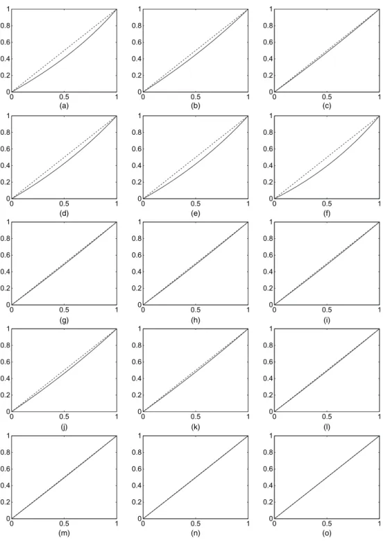
The expression for the Dirichlet process marginals can be found as the limit asa↓0 and usingλ=
1. Fig. 1 shows the relationship betweenρÅand the actual correlationρfor CNGG processes with
different choices of the parameters (including the CDP case in Figs 1(a)–1(c)). The correlation
is close toρÅfor each choice of the hyperparameters with the largest differences for the smaller
values ofaandλ.
For generalM1,M2andM3, these results suggest that increasingM3relative toM1andM2
leads to a larger correlation betweenG1andG2. When q >2, we can always write a pair of
unnormalized distributionsG˜jandG˜k, wherej =k, as
˜
Gj= ˜G.c/+ ˜G.j/,
˜
Gk= ˜G.c/+ ˜G.k/,
where, using I.·/ to denote the indicator function, the L´evy measure of G˜.c/ is given by
{Σp
m=1I.Djm=1,Dkm=1/Mm}η.x/,G˜.j/has L´evy measure{Σpm=1I.Djm=1,Dkm=0/Mm}η.x/
andG˜.k/has L´evy measure{Σpm=1I.Djm=0,Dkm=1/Mm}η.x/. This suggests using the general
approximation
corr.Gj,Gk/≈ M
.c/
√
.M.c/+M.j//√.M.c/+M.k//, .5/
0 0.5 1 0 0.2 0.4 0.6 0.8 1
0 0.5 1
0 0.2 0.4 0.6 0.8 1
0 0.5 1
0 0.2 0.4 0.6 0.8 1
0 0.5 1
0 0.2 0.4 0.6 0.8 1
0 0.5 1
0 0.2 0.4 0.6 0.8 1
0 0.5 1
0 0.2 0.4 0.6 0.8 1
0 0.5 1
0 0.2 0.4 0.6 0.8 1
0 0.5 1
0 0.2 0.4 0.6 0.8 1
0 0.5 1
0 0.2 0.4 0.6 0.8 1
0 0.5 1
0 0.2 0.4 0.6 0.8 1
0 0.5 1
0 0.2 0.4 0.6 0.8 1
0 0.5 1
0 0.2 0.4 0.6 0.8 1
0 0.5 1
0 0.2 0.4 0.6 0.8 1
0 0.5 1
0 0.2 0.4 0.6 0.8 1
0 0.5 1
0 0.2 0.4 0.6 0.8 1
(a) (b) (c)
(d) (e) (f)
(g) (h) (i)
(j) (k) (l)
(m) (n) (o)
Σp
m=1I.Djm=0,Dkm=1/Mm. Therefore, corr.Gj,Gk/increases as the value ofM.c/increases
relative toM.j/andM.k/. Generally, increasingMhleads to increased correlations between all
distributions with a 1 in thehth column ofD.
2.3. Partition probability functions
The previous subsection describes some of the properties of the CNRMI prior. The posterior properties are also interesting and an important step to understanding them is the derivation of the partition probability function which describes the pattern of ties in a sample drawn from distributions with a CNRMI prior. This is known as the exchangeable partition probability function when we have a single sample which can be considered exchangeable. However, the CNRMI prior defines exchangeable sequences in each group but not in the whole sample and so we refrain from using the term exchangeable partition probability function.
Theorem 2. Suppose thatH is a non-atomic probability distribution,ng observations have
been taken in the gth group, there are K distinct values across all samples and nj,i is the
number of times that theith distinct value is observed in the sample for thejth group. Let
f.i/be aq-dimensional vector for which
fj.i/=
1 ifnj,i>0,
0 otherwise,
and letai be the indices of all columns ofDthat can be formed by replacing 0s with 1s in
f.i/(includingf.i/if it is a column ofD). The unknown index of the underlying measure that
generated thejth distinct value is denoted byzj∈{1, . . . ,p}. DefineZ= ×Ki=1ai,
KÅj.z/=#{i|zi=j},
mi= q
j=1
nj,i
and
Iη.n,v/=
Jnexp.−vJ/η.J/dJ:
The partition probability function, describing the probability of obtaining a particular ran-dom partition, is then given by
q
g=1
1
Γ.ng/
z∈Z
.0,∞/qv ng−1 g
p
j=1
MK Å j.z/ j
K
i=1
Iη
mi, q
g=1
Dgzivg
p
j=1 exp
−MjLη
q
g=1
Dgjvg
dv,
wherev=.v1, . . . ,vq/.
Lijoiet al.(2011) derived the same expression (but with rather different notation) for the case
of two groups. In general, the integral in this expression will be difficult to evaluate analytically. However, an analytic expression can be derived in the special case of a CDP prior with two groups.
Corollary 1. If we assume the CDP prior withq=2,p=3 and
D=
1 0 1
0 1 1
,
z∈Z
K
i=1 Γ.mi/
3
j=1
MK Å j.z/ j
Γ.MÅ1+MÅ3−n1/ Γ.MÅ1+MÅ3/
Γ.MÅ2 +MÅ3−n2/ Γ.MÅ2+MÅ3/
×3F2.MÅ3,n1,n2;MÅ1+MÅ3,MÅ2+MÅ3; 1/,
whereqFpis the generalized hypergeometric function andMÅi =Mi+mi.
This result can be interpreted as follows. Using the notation of theorem 1, the distinct values in the first group must be generated from eitherG˜Å1 orG˜
Å
3 and, similarly, the distinct values in
the second group must be generated from eitherG˜Å2 orG˜
Å
3. If these assignments were known
then the partition probability function could be easily calculated. The result in corollary 1 arises from summing this expression over all possible ways that the distinct values could be generated,
which are given by the setZ.
In the special cases of the CDP prior and normalized stable marginals with two groups, Lijoi
et al.(2011) derived expressions for a P ´olya urn representation.
2.4. Modelling of groups
In the simple case with two groups, there are naturally three underlying random measuresG˜Åj
in our model: one modelling the common mass shared between the groups and two for the idiosyncratic components. In cases with more groups, we need to make modelling decisions, which are more fully explored in this subsection. The most flexible models in our class are generated by allocating a separate random measure for modelling the mass that is shared by
each non-empty subset of group distributions. The most complete model forq groups in the
CNRMI class with a givenM,H andηcan thus be defined by takingp=2q−1 and letting the
ith column ofDbe the binary representation ofifor 1i2q−1. For example, ifq=3, then
D=
0 0 0 1 1 1 1
0 1 1 0 0 1 1
1 0 1 0 1 0 1
, .6/
whereG˜Å1,G˜Å2 andG˜Å4 are idiosyncratic components,G˜Å3,G˜Å5 andG˜Å6 are shared by two groups
and G˜Å7 is shared by all three groups. This will be called the saturated model. The levels of
correlation between the distributions can be accommodated by choosing appropriate values of
M1, . . . ,Mpand using approximation (5). Clearly this model becomes increasingly complicated
asqincreases. More parsimonious models can be constructed by removing columns ofDfrom
the saturated model (which is equivalent to setting some Mh to 0). A model with a similar
structure to that of M ¨ulleret al.(2004), with a single common component andqidiosyncratic
components, would use theq×.q+1/-dimensional matrix
D=.1q Iq/,
where1qis aq-dimensional vector of 1s (representing the single common component) andIq
is the.q×q)-dimensional identity matrix. Alternatively, if distributions at different times are
being modelled then a simple model could be defined using
D=.1q Iq R /,
where Ris aq×.q−1/-dimensional matrix for which Rij=1 ifj=iorj=i−1 andRij=
0 otherwise. The model then includes a common underlying measure (in the first column),
idiosyncratic underlying measures (in the next q columns) and underlying random measures
shared by consecutive distributions (in the nextq−1 columns). More problem-specific forms of
0 0.5 1 0
1 2 3 4
0 0.5 1
0 1 2 3 4
(a) (b)
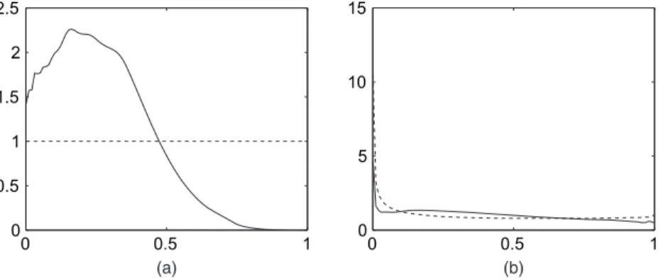
Fig. 2. The prior onρDcorr.G1,G2/for the saturated model withqD2 and (a) a point mass prior onMhand
(b) a shrinkage prior withMhGa.M*=2,φ/whereM*D1 ( ),M*D2 (- - - ) andM*D3.. . . ./ andφD1
where we think thatG1andG2are more related to each other than toG3. A suitable model
would have
D=
1 1 0 0 1
1 0 1 0 1
1 0 0 1 0
,
where the inclusion of the final column allows extra dependence betweenG1andG2.
In practice, we may not have prior information that leads us to consider models that are simpler than the saturated model. We suggest using regularization to avoid overfitting (since the number
of underlying processespgrows quickly withq). A standard approach would be Bayesian variable
selection on the columns ofDfor the saturated model. SettingMh=0 in the L´evy measure of the
underlying measureG˜Åhleads to a degenerate L´evy process with no jumps and so is equivalent to
excluding columnh. We use this formal model selection strategy with a prior point mass at zero.
While always imposing that each group has a properly defined random probability measure (i.e.
Bjas defined in Section 2.1 is non-zero for allqgroups), we assume thatp.Mh =0/=21−q. This
ensures that the prior mass on the correlation between two distributions being 0 does not tend
to 0 or 1 as the number of groups increases. IfMh =0, then it is chosen from an exponential
dis-tribution with mean 1. Under this point mass prior, the probability that the correlation between
any two distributions is 0 depends onqand in the saturated case it is equal to 0.2 whenq=2 and
is approximately 0:2 for largerq. Fig. 2(a) displays the induced prior mass on non-zero values of
ρ, the correlation coefficient betweenG1andG2, whenq=2 andDas in corollary 1, which shows
a dispersed distribution on.0, 1/. In our applications, we shall mostly focus on an alternative
approach and define a prior forMhwhich encourages substantial shrinkage towards zero (this is
similar to the shrinkage prior approach to regression described by Scott and Polson (2011) and Griffin and Brown (2010)). The prior forM1,M2,: : :,Mpis chosen in the following way. The
val-ues ofM1,M2,: : :,Mpcontrol the dependence between distributions and can be chosen to
repre-sent prior beliefs. The additive effect of theMjs is useful here. Suppose that we have one
distribu-tion withMchosen to take the valueMÅ. Moving to two distributions and assuming thatG1and
G2have the same distribution, the saturated model suggests thatM1+M3=MÅandM2+M3=
MÅ, soM1=M2. If we are indifferent between an observation being allocated to a shared cluster
or an idiosyncratic cluster thenM1=M2=M3. Repeated use of this argument allows extension to
any value ofq and suggests thatM1,M2,: : :,Mp are independent andMi∼Ga.MÅ=2q−1,φ/.
withq=2 for various values ofMÅ. All priors are centred on12with the variability decreasing
asMÅincreases. We shall mainly focus onMÅ=1 in our applications. This prior is relatively
flat for correlations larger than 0.1 and has larger mass close to zero. This will lead to some shrinkage of small correlations.
3. Computational methods
This section describes an MCMC sampler for fitting the general mixture model
yg,i∼k.yg,i|θg,i/, i=1, 2, . . . ,ng,
θg,i∼Gg for groupg=1, . . . ,q
and
G1,G2, . . . ,Gq∼CNRMI.M,H,D;η/,
where H andη potentially have hyperparameters which also have priors andH has density
h. The total number of observations isn=Σqg=1ng. First, we describe the algorithm for the
priorMi∼Ga.τi,φi/. The changes to the sampler needed for the prior withp.Mi=0/=p0and
Mi∼Ga.τi,φi/with probability 1−p0are described in Section 3.8.
Walker (2007) introduced a slice sampling method to sample from the posterior of a Dirichlet
process mixture model without truncating its stick breaking representation. Kalliet al.(2011)
developed a more efficient version of this algorithm and extended it to several non-parametric priors. Several slice sampling algorithms for normalized random-measure mixture models were introduced by Griffin and Walker (2011). They showed that their algorithms are competitive with other algorithms for non-conjugate non-parametric mixture models. We shall extend their ‘Slice 1’ algorithm. Importantly, all full conditional distributions involve only a finite number of jumps from the infinite activity L´evy processes but avoid directly truncating smaller jumps of the L´evy process, unlike other methods for non-conjugate NRMI mixtures (Nieto-Barajas and Pr ¨unster, 2009). It should be noted that simply normalizing the jumps of a compound Poisson process does not generate a well-defined non-parametric process. For a single normalized random-measure mixture the posterior is proportional to
p.J/∞
j=1
h.θj/ n
i=1
wsik.yi|θsi/,
where wi=Ji=Σ∞l=1Jl, J=.J1,J2,J3, . . ./ and θ=.θ1,θ2,θ3, . . ./. Griffin and Walker (2011) demonstrated that the following posterior with additional auxiliary variablesu1,u2, . . . ,unand
v1,v2, . . . ,vnand integrating over all jumps smaller thanL=min{ui}is a much simpler form
for computational purposes:
p.J.L//K
j=1
h.θ.L/j /n
i=1
I.ui< Js.L/i /exp
−vi K
l=1
Jl.L/
Eexp
−vi ∞
l=1
Jl.−L/
k.yi|θs.L/i /,
whereJ.L/={Jl|JlL}, which hasKelements,θ.L/is a vector of associated locations,J.−L/= {Jl|Jl< L},u1,u2, . . . ,un>0 andv1,v2, . . . ,vn>0. The expectation can be evaluated by using
the L´evy–Khintchine formula and so
E exp
−v∞
i=1
Ji.−L/
=exp−M L
0
{1−exp.−vx/}η.x/dx
The integral in the exponential is sometimes available in terms of special functions (this is the case for the Dirichlet process) or can be evaluated by using standard quadrature methods.
A latent representation of the posterior of a mixture model using the weights in Section 2 can be derived in a suitable form for computation by introducing latent variables{sj,i}j=1:q,i=1:njwhich
are allocation variables for mixture components whereas{rj,i}j=1:q,i=1:nj allocates each
obser-vation to one ofpunderlying random measuresG˜Å1,G˜
Å
2, . . . ,G˜
Å
p. Thus, the observationyg,i is
assumed to be drawn fromk.·|θr.L/g,i,sg,i/. Using auxiliary variablesuj,1, . . . ,uj,njandvj,1, . . . ,vj,nj
for groupj, the posterior can now be expressed as
q
j=1
Vjnj−1 Γ.nj/
p
i=1
p.Ji.L//
p
i=1 Ki
l=1
h.θi.L/,l / q
j=1 nj
i=1
I.uj,i< Jr.L/j,i,sj,i/ k.yj,i|θ .L/ rj,i,sj,i/
×exp.−VTDJ.+// E[exp.−VTDJ.∞//], .7/
whereJi.L/={Ji,l|Ji,lL}, which hasKielements, andθ.L/i is a vector of associated locations.
We also defineVto be aq-dimensional vector whereVi=Σj=ni1vi,j,J.+/is ap-dimensional vector
with Ji.+/=ΣKi
l=1Ji.L/,l and J.∞/ is a p-dimensional vector whereJi.∞/=Σ∞l=1Ji,l−Σl=Ki1Ji.L/,l .
We can show thatKi∼Pn{Mi
∞
L η.x/dx} (Pn.b/denotes a Poisson distribution with mean
b) and J1,J2, . . . ,JKi are independent conditional on Ki with p.J .L/
i,l /=η.Ji.L/,l /=
∞
L η.x/dx
whereJi.L/,l ∈.L,∞/(so thatJi.L/follows a compound Poisson process). Integrating outuj,iin
expression (7), we obtain
q
j=1
Vjnj−1 Γ.nj/
p
i=1
p.Ji.L//p
j=1 Kj
i=1
h.θj.L/,i /Jj.L/m,i j,i
q
j=1 nj
i=1
k.yj,i|θ.L/rj,i,sj,i/
×exp.−VTDJ.+// E[exp.−VTDJ.∞//],
wheremj,i=#{.l,k/|sl,k=iandrl,k=j, 1knl, 1lq}is the size of the cluster of
obser-vations that are associated withθ.L/j,i.
Each expectation in the product can be evaluated by using the L´evy–Khintchine formula, so
E[exp.−VTDJ.∞//]=exp.−1TpM˜E/˜ ,
whereM˜ is ap×pdiagonal matrix withM˜hh=Mhand, definingD·ias theith column ofD,E˜
is thep-dimensional vector withith element
˜ Ei=
L
0
{1−exp.−VTD·ix/}η.x/dx:
Therefore the latent representation of the posterior retains much of the linearity that is in-troduced in the model. The chain can be initialized in the following way. Choose a
start-ing truncation point L and generate Ki∼Pn{Mi
∞
L η.x/dx}; then J .L/
i are simulated from
the distribution with densityp.Ji.L/,l /=η.Ji.L/,l /=L∞η.x/dxwhereJi.L/,l ∈.L,∞/. The locations
θ.L/
j, 1,θ.L/j, 2, . . . ,θj.L/,Kj are taken to be independent and identically distributed from H and the
latent variablesrj,iandsj,ican be simulated from the discrete distributions
p.rj,i=k/=DjkMk
p
l=1
DjlMl, k=1, 2, . . . ,p,
and
p.sj,i=k/∝k.yi|θ.L/rj,i,k/J .L/
The slice latent variablesuj,iare uniformly distributed on.L,Jr.L/j,i,sj,i/.
In the following steps, we defineJÅj ={Jj,i|mj,i =0}, i.e. the jumps in thejth component
process which have observations allocated to them. Recall thatmj,iis the number of observations
allocated to jumpJj,i. The steps of the Gibbs sampler are described for the case where allMh
have a gamma distribution and are as follows.
3.1. Step 1: split–merge move
The problem of multimodality of the posterior distribution in these models and a computational
solution, a split–merge move, are described in Kolossiatiset al.(2012). In our model, it is useful
to link the underlying measures to their corresponding columns in theD-matrix. For example,
in the saturated model withq=3 andDgiven in equation (6), the underlying random measure
˜
GÅ1 will be referred to as the ‘underlying random measure.0, 0, 1/’. The split–merge move is
performed in the following way. A split move is selected with probability 12; otherwise a merge
move is proposed. An underlying random measuree, a column ofD, is selected at random from
those underlying random measures which have observation allocated to them and a non-empty
mixture componentiÅfromeis selected uniformly at random. If the split move is selected, the
members of the cluster are divided according to their group membership into two clusterse1and
e2. For example, in the saturated model withq=3, if we choosee=.1, 1, 0/the cluster would
be split into a cluster in the underlying measure.1, 0, 0/and a cluster in the underlying measure
.0, 1, 0/. In this case, there is only one possible split. However, if we choosee=.1, 1, 1/, there are three possible splits: clusters in.1, 0, 0/and.0, 1, 1/, clusters in.0, 1, 0/and.1, 0, 1/or clusters in
.0, 0, 1/and.1, 1, 0/. The particular split is chosen uniformly at random from all possible splits. The merge move performs the opposite operation. For this move, a set of allowable underlying measures is defined,C={eÅ|eÅj =0 for alljfor whichej=1}, and an underlying measuree†is
chosen uniformly at random fromC(this happens regardless of whether there are any non-empty
clusters allocated to that measure). One of the non-empty clusters,jÅ, ine†(if any exist) or a
‘null’ cluster is chosen at random with equal probability. A new cluster is then formed in the
underlying random measureecombwhereecomb
i =1 ifei=1 ore†i=1 andecombi =0 ifei=0 and e†
i=0. If a null cluster were selected then the clusteriÅis moved from the underlying measure
etoecomb. Otherwise, clustersiÅ andjÅ are combined to define a new cluster inecomb. Let
.s,r/ and.s,r/be the values of the latent allocation variables before and after making the
move respectively. We assume thatMj∼Ga.τj,φj/. The acceptance probability is calculated by
integrating out the jumps and for the split move has the form
max
1,p.y|s
,r/ p.s,r/
p.y|s,r/ p.s,r/
κKÅ.e/ S.e/
2κKÅ.e1/ M.e1/{KÅ.e2/+1}
,
whereκandκare the number of underlying random measures with observations allocated to
them before and after the move respectively,KÅ.e/andKÅ.e/are the number of non-empty
clusters in the random measureebefore and after the move,M.e/is the size ofCandS.e/is the
number of pairs of underlying measures that can be formed by splittinge. In addition, we can
write
p.s,r/=p
j=1
Γ.τj+KÅj/
.φj+ ˜Aj/τj+K Å j
{i|mj,i =0}
Jjm,ij,i exp.−Jj,iVTD·i/η.Jj,i/dJj,i,
˜ Aj=
∞
0 {
1−exp.−VTD·jx/}η.x/dx:
The move is completed by samplingMfrom its full conditional distribution and then sampling
u,KandJ.
3.2. Step 2: updating V
DefiningA˜=.A˜1, . . . ,A˜p/T, the full conditional distribution ofVjis proportional to
Vjnj−1
Kj
l=1
Jjm,jl,l exp.−Jj,lV T
D·j/dJj,lexp.−1TpM˜A/˜ , Vj>0:
The parameter can be updated by using a Metropolis–Hastings random walk on the log-scale. We also found it useful to updateV Å=Σqj=1Vjconditionally onQ=.V1=V Å, . . . ,Vq=V Å/. The
full conditional distribution ofV Å >0 is
V Ån−1
p
j=1 Kj
l=1
Jjm,jl,l exp.−Jj,lV ÅQ T
D·j/dJj,lexp.−1TpM˜A/:˜
The parameter can be updated by using a Metropolis–Hastings random walk on the log-scale. IfV Åis accepted then eachVjis updated toVjV Å=V Å.
3.3. Step 3: updating M
The full conditional distribution ofMjis proportional to
p.Mj/MjKjexp−Mj
∞
0 {
1−exp.−VjJ/}η.J/dJ
and ifp.Mj/∼Ga.τj,φj/then the full conditional distribution is
Ga τj+Kj,φj+
∞
0 {
1− exp.−VjJ/}η.J/dJ
:
3.4. Step 4: updating u andJ1.L/,J2.L/,. . . ,Jp.L/
This set of full conditional distributions can be updated by using the efficient slice sampling method of Kalliet al.(2011) by integrating outu={uj,i}j=1:q,i=1:nj when updating the jumps.
The update is described for NRMI mixtures by Griffin and Walker (2011) and can be simply extended to our model. The elements ofJÅ1,JÅ2, . . . ,JÅp are simulated first followed by the
ele-ments ofu(which only depends onJkthrough the elements ofJÅk) and finally the other elements
ofJk.L/. The full conditional distribution of the elementJk.L/,l ∈JÅk is proportional to
Jk.L/m,l k,lexp.−Jk.L/,lV T
D·k/η.Jk,l/, Jk.L/,l >0:
The full conditional ofuj,iis uniform on.0,Jr.L/j,i,sj,i/and this allows us to calculateL=min{uj,i}.
Finally, the elements of Jk.L/ for which mk,l=0 can be simulated as follows. First,
simu-lateKk∼Pn{Mk
∞
L exp.−VTD·kx/η.x/dx}; then draw Kk jumps with density proportional
to η.Jk.L/,l/=
∞
L η.x/dx and associate a θ.L/k,l drawn fromH with each jump. Some details of
3.5. Step 5: updatingθ.L/
The elements ofθ.L/ are independent under their joint full conditional distribution, and the
density ofθl.L/,k is proportional to
h.θl.L/,k /
{.j,i/|sj,i=kandrj,i=l}
k.yj,i|θ.L/l,k/,
which is a familiar form that is used in samplers for many infinite mixture models, such as Dirichlet process mixtures.
3.6. Step 6: updating s and r
The latent variablessj,i andrj,i can be updated jointly and drawn from their full conditional
distribution
p.sj,i=kandrj,i=l/∝DjlI.Jl.L/,k > uj,i/ k.yj,i|θl.L/,k /,
where{.l,k/:Jl.L/,k > uj,i}is a finite set.
3.7. Example: (correlated) normalized generalized gamma process marginals
The L´evy density has the form
η.x/= 1 Γ.1−a/x
−1−aexp.−λx/:
The quantities that are used by the MCMC sampler are
Jjm,ij,i exp.−Jj,iVTD·j/η.Jj,i/dJj,i=
1
Γ.1−a/
Γ.mj,i−a/
.λ+VTD·j/mj,i−a,
and the full conditional distribution ofJj,iis Ga.mj,i+a,λ+VTD·j/.
3.8. Markov chain Monte Carlo sampling with a prior point mass at zero forMh
The model whenMhis given a prior with a point mass at zero can be fitted by using an MCMC
sampler which is similar to the one above. A latent variableχ=.χ1,χ2, . . . ,χp/is introduced
to indicate whetherMj=0 (whenχj=0) or Mj∼Ga.τj,φj/is non-zero (whenχj=1). The
differences are described below.
3.8.1. Step 1a: split–merge move
The split–merge move now also includes updating of the latent variableχ. In the split move,
theχs that are associated with the underlying random measures in which the new clusters are
formed are proposed to be both 1. If, following the split move, there are no clusters in the
underlying random measure where the split occurs thenχ is set to 0 or 1 with probability 12
each. Otherwiseχis set to 1. Similarly, in the merge move, the underlying random measure to
which the new cluster is given has a proposedχjequal to 1. The underlying random measures
from which the clusters to be merged are drawn can have theirχs set to 0 if there are no clusters
in that underlying random measure after that move. This again occurs with probability 12. The
p.s,r/=
{j|χj=1}
Γ.τj+KÅj/
.φj+ ˜Aj/τj+K Å j
φτj j Γ.τj/
{i|mj,i =0}
Jjm,ij,iexp.−Jj,iVTD·i/η.Jj,i/dJj,i:
3.8.2. Step 3a: updating M
The full conditional ofMjis Ga[τj+Kj,φj+
∞
0 {1−exp.−VjJ/}η.J/dJ] ifχj=1. Otherwise
Mj=0. In the applications we adoptτj=φj=1 throughout.
4. Comparing distributions
Once we have a posterior distribution on the distributionsG1,G2, . . . ,Gq, it is useful to have
some graphical summaries which help us to understand the differences between distributions. Most simply, we can write
Gi= ¯G+Πi,
where
¯ G=1
q
q
j=1
Gj
is a ‘grand mean’ distribution andΠi=Gi− ¯Gis a signed measure which gives measure zero
toΩand which represents the difference of each distribution from the grand mean. This idea
is similar to the modelling of continuous responses in a one-way ANOVA model. Analogies to higher order ANOVA models are also possible. Suppose that the groups are defined by two covariates (x1andx2) and the distribution for theith level ofx1(i=1, . . . ,n) and thejth level ofx2(j=1, . . . ,m) is represented asGi,j. Then we can decompose
Gi,j= ¯G+Πi·+Π·j+Γi,j, .8/
where
¯ G= 1
nm
n
i=1 m
j=1
Gi,j,
Πi·=1
m
m
j=1
.Gi,j− ¯G/,
Π·j=1
n
n
i=1
.Gi,j− ¯G/
andΓi,j=Gi,j− ¯G−Πi·−Π·j. HereG¯is a probability measure andΠi·,Π·jandΓi,jare signed
measures that put measure 0 onΩ. This separates the effect of leveliofx1averaged over all
levels ofx2, denoted byΠi·, the average effect of leveljofx2(Π·j) and the interaction effects of
combinations of levelsiandjof both variables (Γi,j), giving us a very useful decomposition of
the differences between the distributions.
The summaries described so far allow us to understand and interpret the differences between distributions but we also want to say something meaningful about regions of the support where
the distributions are particularly different. We shall consider a pair of distributionsGiandGj,
and find a partitionP ofΩdefining subsetsPk and an indicator vectord for whichdk= −1
mass thanGi onPk anddk=0 otherwise. The choice ofP andd will be made by specifying
a utility function and finding the partition that maximizes expected utility. The utility func-tion is
U.P,d/=r
k=1
UÅ.Pk,dk/,
whereP1, . . . ,Pr are the elements ofPand
UÅ.P,d/=
⎧ ⎪ ⎨ ⎪ ⎩
Gi.P/−Gj.P/, d= −1,
"
2{Gi.P/+Gj.P/}, d=0,
Gj.P/−Gi.P/, d=1,
where 0< " <2 is chosen to determine the meaning of substantial difference. Increasing values of"lead to a utility function that increasingly favours settingdk=0. To understand the choice
of utility function, consider an elementPkof a fixed partitionP. Then,dk=0 if
|Gi.Pk/−Gj.Pk/| 1
2{Gi.Pk/+Gj.Pk/}
< ":
The left-hand side of the expression is the difference in the mass of the two distributions onPk
divided by the average mass and"is then interpreted as a tolerance parameter which controls
the size of that ratio which constitutes a substantial difference. The expression naturally scales the difference by the mean mass under the two distributions and larger absolute differences will be declared ‘similar’ in areas with larger average mass.
AsU.P,d/is additive over the elements in the partition, maximizing the utility over partitions
is easily done by starting from a very fine partitionP˜and maximizingUÅon each element. Then
we simply join the elements ofP˜ to form the partitionPthat maximizes utility.
5. Applications
The methods that are developed in this paper are illustrated on simulated data, a survival analysis example and an example from efficiency measurement. In all cases, the model with
NGG marginals with λ=1 and unknown other hyperparameters was used. In practice, this
is not a particularly restrictive choice. Writing M= ˇM=λa in equation (3) leads to a process
where λscales the jump sizes and so has no effect on the normalized process (we have also
implemented inference with a prior onλand indeed found that the posterior and prior were
virtually identical). In all applications, we choose the matrixDcorresponding to the saturated
model withp=2q−1 (even for the stochastic frontier example in Section 5.3, whereq=6, so
p=63). Throughout, the prior forawas a uniform distribution on.0, 1/and the prior forMh
was Ga.MÅ=2q−1, 1/which implies that the prior for eachGgis NGG withM∼Ga.MÅ, 1/. We
shall present results forMÅ=1 but also comment on the sensitivity with respect to this choice.
Finally, we also discuss results with a prior point mass at zero forMh.
The MCMC sampler was run with a burn-in of 10000 iterations and a total run of 70000 iterations for all cases. The burn-in period seemed sufficient for the chain to have converged. The split–merge move had an acceptance rate of between 0.1 and 0.2 across the three applications.
5.1. Simulated data
f1.x/=α1N.x|0, 1/+.1−α1/ N.x| −5, 1/
and in the second group from
f2.x/=α2N.x|0, 1/+.1−α2/SkCau.x|2, 2, 0:5/,
where SkCau.·|μ,σ,γ/denotes the skewed Cauchy density function with inverse scale factors
as in Fern´andez and Steel (1998), given by
SkCau.x|μ,σ,γ/= 2
γ+1=γ{Cau.x=γ|μ,σ/ I.x >μ/+Cau.xγ|μ,σ/ I.x <μ/}
using Cau.·|μ,σ/for the standard Cauchy density with locationμand scaleσ, andγ>0 is the
skewness parameter. We adoptγ=0:5, which generates considerable negative skewness, whereas
the mode remains atμ=2.
The model of M ¨ulleret al.(2004) can represent these distributions ifα1=α2but that model
will fit worse as the values ofα1andα2become further apart. We first consider the case with
α1=α2=0:5.
Example 2 extends the first by defining a third group (soq=3 andDhas seven columns) with
observations drawn from the same distribution as the second group, so thatf3.x/=f2.x/. In
this case, we useα1=0:5 andα2=0:9. Each data set was fitted by using the model with NGG
marginals, given by
yg,j ind
∼N.μg,j,σ2g,j/,
.μg,j,σg−,2j/ ind
∼Gg,
G1,G2, . . . ,Gq∼CNGG.M,H,D;a, 1/,
–100 –5 0 5 10
0.1 0.2 0.3 0.4
–100 –5 0 5 10
0.1 0.2 0.3 0.4
–100 –5 0 5 10
0.1 0.2 0.3 0.4
–10 –5 0 5 10
–0.1 –0.05 0 0.05 0.1 0.15
−10 −5 0 5 10
–0.1 –0.05 0 0.05 0.1 0.15
–10 –5 0 5 10
–0.1 –0.05 0 0.05 0.1 0.15
(a) (b) (c)
(d) (e) (f)
Fig. 3. Example 1 (α1Dα2D0:5)—(a)–(c) posterior predictive densities for the two groups ( , group 1;
- - - , group 2) and (d)–(f)f1f¯( ) andf2f¯(- - - -), indicating the area where group 1 has
0 0.5 1 0
0.5 1 1.5 2 2.5
0 0.5 1
0 5 10 15
Fig. 4. Example 1 (α1Dα2D0:5): prior (- - - ) and posterior ( ) densities of (a) the parameteraand
(b) the correlationρfor the NGG prior
withH=N.μ|0,σ2=m0/Ga.σ−2|1, 1/wherem0=0:01.
Some results of fitting the model to data in the first example are shown in Fig. 3. The model estimates the densities well as shown in Figs 3(a)–3(c). The graphs also show partitions of the support found by using the approach in Section 4 for several values of the sensitivity parameter
". The results are reasonably robust to the choice of"with" >0:2 and they indicate that the distributions are substantially different over most of the region shown. Note that the fat tail and left skewness of the distribution of group 2 lead to the latter having relatively more mass for small
x. For"=0:6 we no longer distinguish between the mass that is assigned to the two groups in a region aroundx=0, which, in our view, indicates that this value of"is perhaps a little large. Figs 3(d)–3(f) show the posterior of the differences between the predictive densities and the overall meanfi− ¯fwheref¯=.1=q/Σqg=1fg. It is clear from the definition thatf1− ¯f=−.f2− ¯f /when we have two groups and this is illustrated in the graphs which clearly show where the absolute differences of the densities for the two groups are large.
Fig. 4 shows the posterior densities of the parameteraand the correlationρ=corr.G1,G2/
for the NGG prior. The data favour values ofathat are smaller than 0.5 and indicate a preference
for general NGG marginal processes over the special cases of Dirichlet process or normalized
inverse Gaussian marginals. The posterior distribution ofρ(calculated by using the result of
theorem 1) is not very different from the prior, suggesting that the information in the data about correlation is not strong. The mass close to zero is in line with the fact that the distributions that generated both groups are quite different.
The presented findings correspond toMÅ=1. Results withMÅ=2 andMÅ=3 are very close
in terms of the predictive distributions and show only minor differences for the posterior ona
andρ. In particular, the posterior mass forashifts a little towards zero. Posterior results on
Mh (which are not reported) are only moderately changed by these changes in the prior and
posterior medians ofMhroughly double asMÅchanges from 1 to 3.
If we assign priors with point masses at zero to theMh, we can conduct formal model selection,
as mentioned in Section 2.4. With this prior, predictive distributions are virtually identical to
those reported in Fig. 3 and the posterior forais close as well. Posterior inclusion probabilities
of the components are close to 1 for the shared component, around 0.8 for the idiosyncratic component of the first group and 0.6 for that of group 2.
Fig. 5 shows results of fitting the model to the second example with three groups. The density estimates clearly show the similarities between groups 2 and 3 and the differences with respect
to group 1. The plots offi− ¯fin Fig. 5(b) clearly illustrate the main differences. The posterior
–100 –5 0 5 10 0.1
0.2 0.3 0.4
–10 –5 0 5 10
–0.1 –0.05 0 0.05 0.1 0.15
0 0.5 1
0 0.5 1 1.5 2 2.5
Fig. 5. Example 2 (α1D0:5Iα2D0:9): (a) posterior predictive densities for the three groups; (b) differences
between the predictive densities and the overall mean ( , group 1,f1f¯; - - - , group 2,f2f¯; . . . .,
group 3,f3f¯); (c) posterior density ofa(- - - , prior)
–100 –5 0 5 10
0.1 0.2 0.3 0.4
–100 –5 0 5 10
0.1 0.2 0.3 0.4
–100 –5 0 5 10
0.1 0.2 0.3 0.4 Group 1
Group 2
Group 2 Group 3
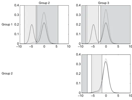
Fig. 6. Example 2 (α1D0:5Iα2D0:9): posterior mean density for the group in the row ( ) and
col-umn (- - - ) and comparison of the distributions with dark and light grey areas indicating more mass for respectively the group in the column and row
Fig. 6 shows the results of making pairwise comparisons for the three groups, using"=0:3.
Changing the value ofMÅfrom 1 to 2 or 3 has very similar effects as in the case of example 1.
Using the alternative prior with point masses at zero forMhleads to virtually identical predictive
results and posterior inclusion probabilities of around 0.95 for the common component and the idiosyncratic component of group 1. The component that is shared by groups 2 and 3 has a posterior inclusion probability of around 0.3, whereas, in line with the generating model, the four other components are assigned little posterior mass (less than 0.2).
5.2. Survival analysis
Doss and Huffer (2003) modelled interval-censored data in survival analysis using the Dirichlet process as a prior for the distribution of the survival times. This application focuses on time to cosmetic deterioration of the breast of women with stage 1 breast cancer who have undergone a lumpectomy under two treatments: radiation and radiation with chemotherapy. There are 46 subjects in the radiation-only group and 48 subjects in the combination group. The data have
been presented in Beadleet al.(1984). The indicatordg,j=1 if thejth person in thegth group
suffers an event (in this case retraction of the breast) before the censoring timeTg,janddg,j=0
otherwise. Ifdg,j=1 then the observation is an intervalAg,jin which the event occured. Doss
and Huffer (2003) assigned a Dirichlet process prior to the lifetime distribution for each group separately. Since the actual survival times are missing (owing to the interval censoring), the posterior will then be a mixture of Dirichlet processes. Denoting the survival time of individual
jin groupgbyτg,j, we extend their approach to the model
I.τg,j∈Ag,j/ifdg,j=1 orI.τg,j> Tg,j/ifdg,j=0,
τg,j ind
∼Gg,
0 20 40 60
0 0.2 0.4 0.6 0.8 1
months 0 20 40 60
0 0.2 0.4 0.6 0.8 1
months 0 20 40 60
0 0.2 0.4 0.6 0.8 1
months
0 20 40 60
–0.2 –0.15 –0.1 –0.05 0 0.05
months 0 20 40 60
–0.2 –0.15 –0.1 –0.05 0 0.05
months 0 20 40 60
–0.2 –0.15 –0.1 –0.05 0 0.05
months
(a) (b) (c)
(d) (e) (f)
Fig. 7. Survival analysis results (- - - , combination group; , radiation-only group) showing (a)–(c) the posterior mean survival functions for the two groups and (d)–(f) the posterior mean forΠ1where the
radiation-only group is coded as group 1 ( , more mass for group 2; , more mass for group 1): (a), (d)
0 0.5 1 0
1 2 3 4
0 0.5 1
0 1 2 3 4 5
0 20 40 60
0 0.2 0.4 0.6 0.8 1
Fig. 8. Survival analysis: prior (- - - ) and posterior ( ) densities of (a) the parameter aand (b) the correlationρ, and (c) the posterior mean and 95% credible intervals of the survival functions for the combination (- - - ) and radiation-only ( ) groups
G1,G2, . . . ,Gq∼CNGG.M,H,D;a, 1/,
whereHis an exponential distribution with mean 1=ξ. The parameterξis given a vague gamma
prior with shape parameter 0.1 and mean 1.
Fig. 7 displays results of the analysis of the clinical trial data. Figs 7(a)–7(c) show that the survival function is similar for the two groups initially but the curves diverge around 16 months with the combination group associated with a much larger number of events. Figs 7(d)–7(f) show the posterior mean of the difference between the survival functions for the groups. They also indicate that the mass is similar until 16 months but then the difference quickly becomes large until the survival functions converge again. The different shades in the graphs also highlight the differences between the distributions for the two groups (rather than the survival functions). The regions that are identified as similar change when moving from"=0:4 to"=0:6 with the latter
having fewer, larger and more connected regions. The results with"=0:6 more clearly highlight
the larger differences in the survival functions, such as the sharp drop in the combination group
around 16 months. Finally, for all values of"the radiation-only group places more mass than
the combination group in the region beyond 45 months.
The posterior distributions ofa andρare shown in Fig. 8, which indicates that the value
a=0 (the Dirichlet process case) is not well supported by the data with a posterior median
close to the normalized inverse Gaussian process (wherea=0:5), but with substantial posterior
uncertainty. The posterior distribution of the correlation parameterρindicates that the groups
are different but do share some common aspects. This can also be seen in Fig. 8(c), where the credible intervals of the survival functions for both groups are closer together for later survival times than in the independent Dirichlet process analysis of Doss and Huffer (2003). This is in line with the fact that more patients are censored in the radiation group, which shrinks the credible interval towards that for the combination group. The effect of NGG rather than
Dirichlet process marginals (largerainduces more small jumps and smoother distributions) is
difficult to evaluate on the basis of mean survival functions.
Changing the prior onMhby varyingMÅto 2 and 3 has no discernible effect on the predictive
distributions and very little effect on the posterior foraandρ. Posterior distributions forMh
are somewhat affected by this, with posterior medians increasing by a factor of about 2 asMÅ
is increased from 1 to 3.
If we use the point mass prior onMh, we find again that the predictive distributions are
0 0.5 1 0
1 2 3
0.4 0.6 0.8 1
0 2 4 6 8
(b) (a)
Fig. 9. Stochastic frontier analysis: (a) posterior ( ) and prior (- - - ) densities ofaand (b) the density of the posterior mean of the average efficiency distribution with an NGG prior
5.3. Stochastic frontier analysis
Stochastic frontier analysis is a popular method in econometrics for estimating the efficiency of firms. We shall consider an application to the efficiency of US hospitals by using data that have
previously been analysed by Koopet al.(1997). It is assumed that all hospitals operate relative
to a common cost frontier, which represents the minimum cost of performing the functions of that hospital (including operations, patient care, etc.). Inefficiency can then be measured by how far a hospital operates above the optimal cost level that is given by the frontier. The costs are observed for the hospitals over a number of years. The model is written in terms of log-cost
Cg,j,tfor thejth hospital in thegth group at thetth time point
Cg,j,t=α+xTg,j,tβ+ug,j+"g,j,t,
wherexg,j,tare variables used to define the frontier for hospitaljin groupgat timet,ug,j>0 is
the inefficiency for hospitaljin groupgand"g,j,tare mutually independent measurement errors
which will be assumed to be normally distributed with mean 0 and varianceσ2. The model
assumes that the efficiency of hospitals is constant over the observed time period (which is a
common assumption in the applied literature). The efficiency for hospitaljin groupgis defined
to be exp.−ug,j/.
The main focus of this type of analysis is the estimation of the hospital efficiencies exp.−ug,j/.
A Bayesian non-parametric analysis of the stochastic frontier model is described by Griffin and Steel (2004) who assumed a Dirichlet process prior for the inefficiency distribution and used the same data set. The model used in the present paper is
Cg,j,t ind
∼N.α+xTg,j,tβ+ug,j,σ2/,
ug,j ind
∼Gg
G1,G2, . . . ,Gq∼CNGG.M,H,D;a, 1/,
whereα,β andσ2are given the priors that were described by Griffin and Steel (2004) andH
is an exponential distribution with mean 1=ξ, whereξis given an exponential prior with mean
−1=log.rÅ/, so thatrÅis the prior median efficiency. In this examplerÅis subjectively chosen
to take the value 0.8. Fig. 9 shows some posterior results of extending the model of Griffin and Steel (2004) using the prior that was developed in this paper for just one group. The posterior
0.4 0.6 0.8 1 0
2 4 6 8
0.4 0.6 0.8 1
0 2 4 6 8
0.4 0.6 0.8 1
0 2 4 6 8
0.4 0.6 0.8 1
0 2 4 6 8
0.4 0.6 0.8 1
0 2 4 6 8
0.4 0.6 0.8 1
0 2 4 6 8
(b) (c)
(a)
(e) (f)
(d)
Fig. 10. Stochastic frontier analysis—density of the posterior mean of the efficiency distribution for each hospital type with a CNGG prior: (a) for profit, low SPR; (b) non-profit, low SPR; (c) government, low SPR; (d) for profit, high SPR; (e) non-profit, high SPR; (f) government, high SPR
distribution with just a single group (averaged over all hospital types) has three internal modes at roughly 0.65, 0.7 and 0.8 and a further mode at 1, which is quite in line with the results for the efficiency that were obtained in Griffin and Steel (2004) based on all the data. We now use information about the type of hospital expressed by two discrete covariates: the ownership status of the hospital (for profit, non-profit and government) and a quality factor in terms of the staff–patient ratio SPR (low or high). The precise definition of these covariates is described
in Koopet al.(1997).
Fig. 10 shows the density corresponding to the posterior mean of the efficiency distribution within each group defined by these two covariates. It should be noted that these densities exist
since the kernel is continuous inug,jandhis continuous, which implies that the posterior means
ofG1, . . . ,Gpare continuous. For comparison, an analysis using a product of Dirichlet processes
was provided by Griffin and Steel (2004). They specified separate non-parametric inefficiency distributions for each group, which are linked only indirectly by the centring distribution, which is allowed to depend on firm characteristics, and a common mass parameter. The dependent non-parametric prior that was developed in the present paper leads to predictive distributions which vary substantially less between groups, illustrating the model’s ability to borrow information effectively. This is particularly important in this application where group sizes are quite small, ranging from 20 to 141. All distributions are multimodal with most densities having modes at roughly 0.7 and 0.8 (and at 1). However, the sizes of the modes differ between the groups.
The decomposition in equation (8) more clearly shows the differences and similarities between the distributions. Fig. 11 shows the densityπi·of the posterior mean ofΠi·,π·jof the posterior mean ofΠ·j, andγi,j of the posterior mean ofΓi,j(again, these densities exist). Theπs show