warwick.ac.uk/lib-publications
A Thesis Submitted for the Degree of PhD at the University of Warwick
Permanent WRAP URL:
http://wrap.warwick.ac.uk/89458
Copyright and reuse:
This thesis is made available online and is protected by original copyright.
Please scroll down to view the document itself.
Please refer to the repository record for this item for information to help you to cite it.
Our policy information is available from the repository home page.
modelling for biomedical systems
by
Yan ZHANG
张
张
张
雁
雁
雁
Thesis
Submitted to The University of Warwick
for the degree of
Doctor of Philosophy
The School of Engineering
I, Yan Zhang, declare that this thesis titled, ’Variational Bayesian data driven modelling
for biomedical systems’ and the work presented in it are my own. I confirm that:
This work was done wholly or mainly while in candidature for a research degree
at this University.
Where any part of this thesis has previously been submitted for a degree or any
other qualification at this University or any other institution, this has been clearly
stated.
Where I have consulted the published work of others, this is always clearly
at-tributed.
Where I have quoted from the work of others, the source is always given. With
the exception of such quotations, this thesis is entirely my own work.
I have acknowledged all main sources of help.
Where the thesis is based on work done by myself jointly with others, I have made
clear exactly what was done by others and what I have contributed myself.
Signed:
Date:
anyone. ”
Physiological systems are well recognised to be nonlinear, stochastic and complex. In
situations when only one time series of a single variable is available, exacting useful
information from the dynamic data is crucial to facilitate personalised clinical decisions
and deepen the understanding of the underlying mechanisms. This thesis is focused
on establishing and validating data-driven models, that incorporate nonlinearity and
stochasticity into the model developing framework, to describe a single measurement
time series in the field of biomedical engineering. The tasks of model selection and
pa-rameter estimation are performed by applying the variational Bayesian method, which
has shown great potential as a deterministic alternative to Markov Chain Monte Carlo
sampling methods. The free energy, a maximised lower bound of the model evidence, is
considered as the main model selection criterion, which penalises the complexity of the
model. Several other model selection criteria, alongside the free energy criterion, have
been utilised according to the specific requirements of each application. The
method-ology has been employed to two biomedical applications. For the first application, a
nonlinear stochastic second order model has been developed to describe the blood
glu-cose response to food intake for people with and without Diabetes Mellitus (DM). It was
found that the glucose dynamics for the people with DM show a higher degree of
non-linearity and a different range of parameter values compared with people without DM.
The developed model shows clinical potential of classifying individuals into these two
groups, monitoring the effectiveness of the diabetes management, and identifying people
with pre-diabetes conditions. For the second application, a linear third order model
has been established for the first time to describe post-transplant antibody dynamics
after high-risk kidney transplantation. The model was found to have different ranges of
parameter values between people with and without acute antibody-mediated rejection
(AMR) episodes. The findings may facilitate the formation of an accurate pre-transplant
risk profile which predicts AMR and allows the clinician to intervene at a much earlier
This thesis would not have been possible without the kind help and support that I have
received during the course of my Ph.D from my supervisors, colleagues, family, and
friends, without whom I would not be able to overcome the frustrations and
difficul-ties along the way. For this I am eternally indebted and it is a pleasure to have the
opportunity to express my gratitude to them all.
My sincerest gratitude goes to my supervisor, Dr. Natasha Khovanova, for her
continu-ous guidance and support throughout four years, with more scheduled and unscheduled
meetings than I can count. I am deeply grateful that she offered me this great
opportu-nity to do research in the field of biomedical engineering which I feel passionate about,
and introduced me to the inverse problem and the Bayesian inference methods that
have intrigued me ever since. During the years, she has offered a tremendous amount of
time and energy to advise me and discuss the research problem, and to teach and revise
my writing meticulously. Without her, this thesis would never have been completed.
I would also like to express my gratitude to my second supervisor, Dr. Neil Evans,
and Dr. Igor Khovanov, for all the inspirational ideas, valuable advice and kind help
that they have given me over the years. I would like to thank all the collaborators with
whom I have worked on my projects. I enjoyed working with them and I have learnt a
lot through many meetings and conversations with them.
I am indebted to my good friends, Anup Das, Felicity Kendrick, and Magnus Tr¨ag˚ardh,
who have contributed and extended their appreciable help to discuss, proofread, and
re-proofread the details in this thesis, which I shall never forget. My thanks also go to
all my labmates who are and were in Warwick Engineering in Biomedicine, from whom I
have received incredible support and encouragement, their friendship and company have
made this Ph.D much more fun and enjoyable than it would have been without them.
Words fail me to express my deepest gratitude to my parents, Zongtao Zhang and
Fangming Lin, for their unconditional love, selfless support and incredible patience, and
my dog, Xiaohu, for being the best companion for my parents when I am far away in
another country.
Declaration of Authorship i
Abstract iii
Acknowledgements iv
List of Figures viii
List of Tables xi
Abbreviations xii
Symbols xiv
Disseminations xvi
Dedication xix
1 Introduction 1
1.1 Overview . . . 1
1.2 Aim and objectives . . . 8
1.3 Overview of the thesis structure. . . 10
2 Methodology 11 2.1 Model specification . . . 11
2.1.1 Model formulation using ordinary differential equations (ODE) . . 12
2.1.2 Model formulation using stochastic differential equations (SDE). . 14
2.2 Model selection and parameter estimation . . . 15
2.2.1 Maximum Likelihood and Maximum-a-Posteriori . . . 17
2.2.2 Full Bayes’ method . . . 18
2.3 Variational Bayesian scheme. . . 21
2.3.1 Kullback–Leibler divergence and free energy. . . 22
2.3.2 Parameter and state estimation . . . 25
2.3.3 Iterative updating rule for hyperparameters, parameters and the states . . . 26
2.3.4 Free energy decomposition. . . 31
2.4 The criteria for model selection . . . 37
2.5 Priors and hyperpriors . . . 43
2.6 Structural identifiability . . . 47
2.7 Parameter sensitivity analysis . . . 52
2.8 Illustrative example of the use of the VB toolbox . . . 54
2.8.1 The toy model . . . 55
2.8.2 The choice of priors . . . 56
2.8.2.1 Initial default setting of priors and hyperpriors . . . 57
2.8.2.2 Select the mean vector of the prior distribution for the parameters . . . 59
2.8.2.3 Select the variances of prior distributions for the param-eters. . . 61
2.8.2.4 Select the hyperpriors for the hyperparameters . . . 63
2.9 Chapter summary . . . 68
3 Post-prandial glucose dynamics 70 3.1 Introduction. . . 71
3.2 Data description . . . 76
3.3 Model and Methods . . . 80
3.3.1 Model formulation . . . 80
3.3.2 Model selection and parameter inference . . . 82
3.3.3 Model selection criteria . . . 85
3.4 Results and Discussions . . . 85
3.4.1 Model selection and parameter inference . . . 85
3.4.2 Structural identifiability and parameter sensitivity . . . 91
3.4.3 Parameter comparison between the groups. . . 93
3.4.3.1 Coefficients of functionf0 and undamped frequency . . . 94
3.4.3.2 Coefficients of functionf1 and damping . . . 94
3.4.3.3 Noise . . . 97
3.4.4 Impulsive force . . . 98
3.4.5 Link between the data-driven model and physiological models. The signs of pre-DM . . . 100
3.5 Conclusions and limitations of the study . . . 103
4 Post-transplant antibody dynamics 105 4.1 Introduction. . . 106
4.2 Data description and visual analysis of dynamic patterns. . . 110
4.3 Models and methods . . . 113
4.3.1 Data fitting and model selection . . . 113
4.3.1.1 Exponential fitting. . . 113
4.3.1.2 Form of the model: linear/nonlinear and stochastic terms114 4.3.2 Model and parameter identification. . . 115
4.3.3 Model selection criteria . . . 116
4.4 Results and Discussions . . . 117
4.4.1 Model selection . . . 117
4.4.1.2 Deterministic versus stochastic . . . 121
4.4.1.3 Nonlinear versus linear . . . 122
4.4.2 Model validation . . . 123
4.4.3 Structural identifiability and parameter sensitivity . . . 125
4.4.4 Analysis of the inferred parameters . . . 127
4.4.4.1 Comparison of deterministic parameters . . . 127
4.4.4.2 Comparison of stochastic parameters . . . 129
4.4.5 Eigenvalues . . . 130
4.5 Conclusions . . . 133
5 Conclusions and future work 135 141
2.1 Approximation of the parameter distribution of P based on two K-L di-vergence measures; q1(x) is based on KL[QkP] and q2(x) is based on
KL[PkQ]. . . 23 2.2 One iteration cycle of the VB algorithm. In each step, the probability
distribution of theith componentqi (i= 1,2,3,4,5) is optimised to max-imise the free energy F while keeping the probability distributions of the other components fixed. The lower bound of the log-evidence, i.e. the free energy, is guaranteed to increase (or stay unchanged) during each step. The mark ∗ indicates that the probability distribution has been updated. 27 2.3 Illustration of the model M. yt is the measurement point at time t, and
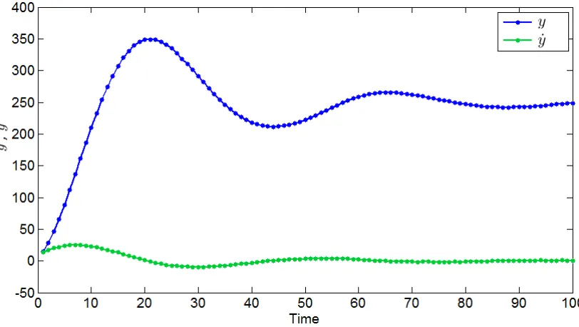
xtis the state vector of the system at timet. θis the parameter vector of the system equation (2.2). αη is the precision of the system noise andαε is the precision of the measurement noise, ut is the input of the system at timet. . . 28 2.4 Simulated time series from the toy model. . . 56 2.5 The correlations between the parameters θ1,θ2, θ3 and the initial
condi-tions x0, ˙x0. The correlation between θ2 and θ3 is 0.97, between θ1 and
θ2 is 0.54, and between θ1 and θ3 is 0.60. . . 59
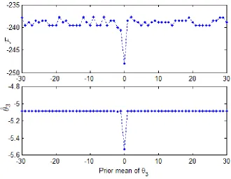
2.6 Free energy and posterior means of θ3 using different prior means ofθ3. . 60
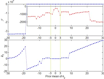
2.7 Free energy and posterior means of θ2 using different prior mean values
of θ2 . . . 61
2.8 Free energy and posterior means of θ1 using different prior means ofθ1 . . 62
2.9 Free energyF and RMSEΣ with the variance of the prior distribution for
all three parameters 10jI3 changing from j=−2 to j= 8. . . 63
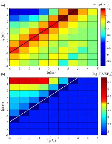
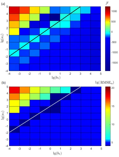
2.10 Probability density distribution of the precision of the noise . . . 64 2.11 (a)The value of free energy and (b) RMSEα for different combinations of
the shape a2 and rate b2 hyperpriors for the measurement noise. Note
that the figure is shown in log-scale (with a base of 10). All the free energy values F in this graph are negative, so the logarithm of the free energy is calculated by −lg(|F |). . . 65 2.12 (a)The value of free energy and (b) RMSEα for different combinations of
the shapea2 and rateb2 hyperpriors for the system noise. Note that the
figure is shown in log-scale (with a base of 10). . . 67
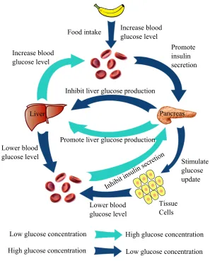
3.1 Simple illustration of the glucose - insulin feedback system. . . 72
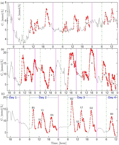
3.2 Example subcutaneous glucose time series G of a participant from (a) the control group (b) the T1D group (c) the T2D group. The solid grey curves represent the measured glucose values and the dots are the values used for modelling of single postprandial peaks. The solid and dashed vertical lines correspond to midnight (0 hours) and 6 am respectively. The first several hours of data in Day 1 (to the left from the first solid vertical lines) were excluded from the modelling due to the adjustment period of the CGM system. ‘B’ indicates breakfast, ‘S’ indicates snack, ‘L’ indicates lunch, ‘D’ indicates dinner. . . 79 3.3 Typical outcome for one peak (the sixth peak in Fig. 3.2 (b)) fitting by
four models. . . 86 3.4 The fitting results are shown for: (a) a peak of a T2D profile; (b) a peak
of a T1D profile. The lines are simulated deterministic solutions using the inferred parameters for MLand M2. . . 89
3.5 Glucose time series G of a T2D subject. The solid grey curves represent the measured glucose values and the dots are the values used for modelling of single postprandial peaks. The glucose time series corresponding to responses to food intake during breakfasts are indicated by dark black crosses. The solid and dashed vertical lines correspond to midnight (12 am) and 6 am respectively. . . 91 3.6 The fitting results are shown for three peaks (represent breakfasts) of a
T2D profile (as in Fig. 3.5) in three consecutive days from (a) – (c). The free energy value of ML is denoted as FML, and the free energy value of M2 is denoted asFM2. . . 92 3.7 Boxplots for parameter √θ1/2π obtained from (a)ML and (b)M2. Note
that the denominator 2πis to convert the units from [radian/min] to [min−1] 95 3.8 Boxplots for the damping coefficients ζ= θk
2×√θ1 obtained from ML. . . . 95 3.9 Boxplots for parameters: (a)θk inML; (b)θk0 inM2; (c) θk1 inM2; (d)
θk2 inM2. . . 96
3.10 Boxplots for intensities of system noiseIε in (a) ML and (c) M2, and of
measurement Iη noise in (b)ML and (d)M2 . . . 97
3.11 Boxplots for the initial force parameters F compared between the three groups.. . . 99 3.12 Boxplots for the food impact force F compared (a) between patient No.
15 and the rest of the T2D group; (b) among the subjects in the T2D groups.. . . 100 3.13 The dotted line is the simulated time series from the maximal model
for a non-DM case without any signs of DM and the solid line is the deterministic solution using the parameter values inferred from modelML.101 3.14 Boxplots for (a) θk0 and (b) θ1 for all measured peaks fitted by ML in
our cohort of participants. Horizontal lines mark θM M
k0 and θM M1 for no
signs of DM (upper dashed green line), low insulin sensitivity (middle solid line) and impaired β-cell function (lower dashed pink line) cases. . . 103
4.2 Measured time series illustrating individual DSA changes in the AMR group. Markers correspond to each measurement point. MFI=mean flu-orescence intensity. . . 112 4.3 Typical fitting results compared among the three models M1 – M3 for
(a) B60 (case 52) for a patient from the no-AMR group; (b) HLA-DRB3*01 for a patient (case 14) from the AMR group; (c) HLA-A32 for a patient (case 16) from the AMR group; (d) HLA-A2 for a patient (case 17) from the AMR group. The measured values are indicated by circles. . 119 4.4 Boxplot of the difference between the NRMSE of M2 and NRMSE of M3. 121
4.5 Fitting comparison betweenM3S andM3 for the time series in Fig. 4.3 (b).122
4.6 Fitting results compared between the two nonlinear models N M1 and
N M2 and the linear model M3 for the time series shown in Fig. 4.3 (c).
The measured values are indicated by circles. . . 124 4.7 NRMSE value of the errors between the observations and the estimated
values by M2 and M3 . . . 125
4.8 Boxplot for the inferred parametersθ0,θ1,θ2,θ3 . . . 127
4.9 Boxplot for the settling values compared between no-AMR and AMR groups128 4.10 Phase portraits of the three dimensional system for two DSA time series,
(a) from a patient in the AMR group and (b) from a patient in the no-AMR group. The time difference between two consecutive markers is one day. . . 131 4.11 Boxplot for (a) the larger real part of the eigenvalues; (b) the smaller real
part of the eigenvalues; (c) the imaginary part of the eigenvaluesλ2,3; (d)
2.1 Bayes factor compared between models M1 and M2 . . . 42
2.2 Summary of the parameter settings for the time series simulated by the toy model . . . 56
3.1 Biometric indices, treatment regimens, HbA1c values and corresponding estimated average blood glucose levels of participants. . . 78 3.2 Four model candidates for fitting . . . 83 3.3 Free energy of ML, denoted as FML, for different hyperprior settings of
the precision of system noise. . . 87 3.4 Free energy of M2, denoted as FM2, for different hyperprior settings of
the precision of system noise. . . 87 3.5 Inference results of the parameters for the example shown in Fig. 3.3 . . . 88 3.6 Summary of peak fitting using ML andM2 . . . 90
3.7 Summary of the parameter sensitivities for ML and the range of RMSE with 1% parameter perturbation . . . 93 3.8 Summary of the parameter sensitivities for M2 and the range of RMSE
with 1% parameter perturbation . . . 94
4.1 Summary of the free energy and the NRMSE values for three models of different order corresponding to the four example datasets in Fig. 4.3. . . 120 4.2 Summary of the parameter sensitivities forM3 . . . 127
AIC AkaikeInformationCriterion
AICc Corrected AkaikeInformation Criterion
AiT Antibody incompatible Transplantation
AMR Antibody MediatedRejection
AR AutoRegressive
AWGN AdditiveWhite Gaussian Noise
BIC Bayesian InformationCriterion
CGM Continuous Glucose Monitoring
CV Coefficient of Variability
DSA DonorSpecificAntibody
DM DiabetesMellitus
GOF GoodnessOf Fit
HLA Human LeukocyteAntigen
K-L Kullback -Leibler
LS LeastSquare
MAP MaximalA Posteriori
MCMC Markov ChainMonte Carlo
MFI Mean FluorescenceIntensity
ML Maximum Likelihood
M M MaximalModel
NRMSE Normalised Root MeanSquare
ODE Ordinary Differential Equation
RMSE Root MeanSquareError
SDE StochasticDifferential Equation
SISO SingleInputSingleOutput systems
SMC SequentialMonte Carlo
T1D Type 1 Diabetes
T2D Type 2 Diabetes
A State matrix
B Input matrix
B1,2 Bayes factor in favour of model M1 over model M2
C Output matrix
C Constant
δ(t) Dirac delta function
E Energy term in the calculation for free energy
fi Polynomial functions in the system equation
F Food impact force
F Variational free energy, or free energy for short in this thesis
F I Fisher information matrix
g Measurement function in the measurement equation
G Glucose concentration
Ga Gamma distribution
Gb Glucose basal level
H Shannon entropy, or entropy for short in this thesis
H Hessian matrix
I Variational energy
Iη Intensity of system noise
Iε Intensity of measurement noise
k Dimension of the parameter space, or the number of the parameters
KL(PkQ) Kulback-Leibler divergence from probability density functionq(x) to p(x)
KLr Relative Kulback-Leibler divergence
M Model
N Normal distribution or Gaussian distribution
p(·) Normalised probability density function
P(·) Unnormalised likelihood function
P(M|y) Marginal likelihood or model evidence
P(y|θ, M) Conditional likelihood of obtaining measurement y
lg Logarithm with a base of 10
log Natural logarithm
logP(y|M) Log-evidence of the model
logP(y|M,θ) Log-likelihood of the model
q(·) Approximated probability density function ofp(·)
h·ip Expectation of ·with respect to the probability distribution p
S Self-information
SIθi Sensitivity index for the parameterθi
ut Input at timet
x State vector
x(ti) ith derivative of the states at time t
y Measurement vector
yt Measurement data point at timet
yt(i) ith derivative of the measurement at time t
αη Precision of the system noise
αε Precision of the measurement noise
γ(·) Gamma function
ση Standard deviation of the system noise
σε Standard deviation of the measurement noise
Σ Covariance matrix
ηt System noise at timet
εt Measurement noise at timet
Θ All the components that requires iterative updating in the VB scheme
θ Parameter vector
θ(i) Thei the sample ofθ
φ Parameter vector of the measurement equation
Results of this research have been disseminated in 6 publications and at 10 conferences
as below:
List of Publications
1. Y. Zhang, D. Briggs, D. Lowe, D. Mitchell, S. Daga, N. Krishnan, R. Higgins and N.
Khovanova, “A new data-driven model for post-transplant antibody dynamics in
high risk kidney transplantation”, doi: 10.1016/j.mbs.2016.04.008, Mathematical
Biosciences, 2016, in press
2. Y. Zhang, T. A. Holt, and N. Khovanova, “A data driven nonlinear stochastic
model for blood glucose dynamics”,Computer Methods and Programs in Biomedicine,
vol. 125, pp. 18–25, 2015
3. Y. Zhang, D. Lowe, D. Briggs, R. Higgins, and N. Khovanova, “Novel
data-driven stochastic model for antibody dynamics in kidney transplantation”,IFAC–
PapersOnLine, vol. 48, no. 20, pp. 249–254, 2015
4. N. Khovanova, Y. Zhang, and T. A. Holt, “Generalised stochastic model for
char-acterisation of subcutaneous glucose time series”,IEEE-EMBS International
Con-ference on Biomedical and Health Informatics (BHI), pp. 484–487, June 2014
5. Y. Zhang and N. Khovanova, “A novel stochastic model of postprandial blood
glucose time series”, PGBiomed/ISC–2014: 8th IEEE EMBS International UK
& Republic of Ireland Postgraduate Conference on Biomedical Engineering and
Medical Physics, University of Warwick, 2014
6. Y. Zhang, N. Khovanova, and T. A. Holt, “Inference of stochastic nonlinear
equa-tions for characterisation and prediction of prandial blood glucose levels”,ENOC
2014: Proceedings of 8th European Nonlinear Dynamics Conference, Institute of
Mechanics and Mechatronics, Vienna University of Technology, July 2014
List of posters and presentations in conferences
1. Poster presentation (Best Poster Award): N. Khovanova, Y. Zhang, D. Lowe, D.
Briggs, and R. Higgins, “Dynamic Model for the Evolution of Donor Specific (DSA)
Antibodies after HLA Antibody Incompatible (HLAi) Kidney Transplantation”,
BSHI 2015: British Society for Histocompatibility and Immunogenetics Annual
Conference, Cambridge, September, 2015
2. Poster presentation: Y. Zhang, D. Lowe, D. Briggs, R. Higgins and N. Khovanova,
“Variational Bayesian state-space model for antibody dynamics after kidney
trans-plantation”,3rd Meeting on Statistics, Athens, Greece, June, 2015
3. Oral presentation: Y. Zhang, D. Lowe, D. Briggs, R. Higgins, and N. Khovanova,
“Novel data driven stochastic model for antibody dynamics in kidney
transplanta-tion”,IFAC2015: 9th IFAC Symposium on Biological and Medical Systems, Berlin,
Germany, August, 2015
4. Oral presentation: Y. Zhang, “Variational Bayesian inference method in
stochas-tic modelling of subcutaneous glucose concentration”, DINSTOCH: Workshop on
Statistical Methods for Dynamical Stochastic Models, University of Warwick, UK,
September, 2014
5. Oral presentation: Y. Zhang, N. Khovanova: “Variational Bayesian analysis of
blood glucose time series”, SCCS2014: the Student Conference on Complexity
Science, Brighton, UK, August 2014
6. Poster presentation: “Inference of stochastic nonlinear equations for
characterisa-tion and prediccharacterisa-tion of prandial blood glucose levels” ENOC2014: 8th European
Nonlinear Dynamics Conference, Vienna, Austria, July, 2014
7. Member of the organising committee and oral presentation: Y. Zhang, N.
8th IEEE EMBS UK & Republic of Ireland Postgraduate Conference on Biomedical
Engineering and Medical Physics, University of Warwick, UK, July 2014
8. Poster presentation (Best Poster Prize Runner-up): Y. Zhang,
“Stochas-tic modelling of subcutaneous glucose concentration after meals”, [id]2Ox
inter-disciplinary inter-DTC Student Conference, Oxford, June, 2014
9. Oral and poster presentation: Y. Zhang, “A data-driven approach for blood glucose
modelling”,Simplifying Assumptions in Models of Complex Systems: Break, Make,
Justify, University of Birmingham, UK, May, 2014
10. Poster presentation (Best Poster Presentation Award): Y. Zhang, N.
Kho-vanova, and T. A. Holt, “Stochastic modelling of subcutenious glucose levels
by variational Bayesian inference approach”, Annual Postgraduate symposium,
Introduction
1.1
Overview
Extracting useful information from limited clinical data has always been one of the
main focuses of biomedical research. Clinicians need to make decisions – sometimes
life-changing ones – for individual cases based on the available data, which can often be
sparse and noisy [1]. Clinical data can broadly be split into two categories: one type
characterises the static properties such as age, gender, etc., and the other type
char-acterises the dynamic properties of how the physiological system evolves. Whilst the
first type of data is usually statistically analysed through data-mining techniques, the
second type is often limited to monitoring purposes after certain clinical interventions or
treatments. However, the dynamic response of the physiological system after a clinical
intervention or treatment carries essential information about possible clinical outcomes,
and therefore should be extracted and analysed to help the clinicians provide improved
prevention and screening, diagnosis, prognosis, and/or predictions of response to
treat-ment or clinical intervention [2–4]. Various mathematical models have been established
to describe, interpret, or predict the dynamic behaviours in clinical data [5–7] to obtain
two essential pieces of information: 1) the common patterns shown by different groups of
patients and 2) the distinctive features that only belong to an individual. However, when
knowledge of the underlying physiological system is limited, it is not straightforward to
establish a model that is capable of classifying and recognising patterns in clinical data.
There are two fundamental approaches to developing a mathematical model for
describ-ing the dynamics of physiological systems [8], with the purpose of obtaining control of
the physiological system to external stimuli. The first approach is based on the
under-standing of the physiological processes that generate the measured data, which are often
referred to as physiological or mechanistic models. Depending on the purpose of the
model, this approach can be used to establish models at the molecular, cellular, tissue
or organ scale with parameters that have direct physiological interpretations [9]. The
process can be time-consuming, may be even impossible in practice, since it requires
knowledge at a detailed level about the system’s structure and all its parameters. The
second approach is focused on describing the measurement data without taking into
account explicit knowledge of the physiological processes underneath, which are often
referred to as data-driven models. In this case, the system’s internal structure is
con-sidered as a black box and the only available information about the system is given by
its measured inputs and outputs, and the model structure needs to be flexible enough
to capture the variations in the data [10]. Data-driven modelling is best implemented
when it can be based on the use of inexpensive accessible measurement data to produce
parsimonious models [11,12]. Choice between these two approaches depends on the aim
of the research, the level of the understanding of the system, and the availability of the
data. The mechanistic approach is better for gaining insight into the working
princi-ple of a system, but when the underlying system is not well-understood, establishing a
data-driven model may help determine critical characteristics that can provide valuable
information for later establishing the mechanistic models [13].
There are several difficulties regarding establishing the first type of model for
physiolog-ical systems. 1) The most challenging part is to formulate the extraordinary complexity
of a physiological system that is the culmination of millions of years of evolution. A
sys-tem is defined as complexwhen the interactions between the components of the system
generate properties that cannot be reduced to its subunits [14]. In physiological systems,
new properties have been created as a consequence of the entwined feedback loops that
keep humans within the narrow bounds needed for survival [9]. For example, it may be
possible for the human body to survive the removal of certain parts by a spontaneous
self reorganisation of the system, such as the reshaping of the nervous system following a
severe injury, known as brain plasticity. However, a highly intertwined system structure
physiological system is handled in nature through multiple feedback mechanisms. This
also presents a challenge to system identification due to intrinsic couplings between the
variables and strong limitations to the exogenous excitation. 2) It is a formidable task
to identify all the parameters in physiological models [15]. Any physiological model that
is even approximately realistic will have a large number of parameters [16]. Researchers
commonly try to determine the values of these parameters given only one measurement
time series, such as the concentration of a certain type of blood cell, the electrical
activ-ity of the heart over a period of time (also known as electrocardiography), the human
breath rate or the heart rate time series, etc. [17,18]. In many cases, it is impossible
to estimate these parameters, even with perfect data, due to lack of structural
identi-fiability. In cases where the parameter can be estimated in theory, it can still remain
statistically challenging, especially in the case where the number of the observation data
points in the time series and the number of the parameters are comparable [16]. When
certain physiologically based variables in the model are inaccessible, it might be possible
to identify these variables in animals where more invasive studies can be conducted [19].
However the translation between human and animal parameters is not as simple as linear
scaling [20]. 3) Another important problem is the limited data available for personalised
modelling. In clinical applications, individualised models are required for personalised
patient care, but many physiological models use a single set of parameters representing
the ‘average person’ [16]. However, reliable data acquired through minimally invasive
techniques for each patient still remain scarce [21]. 4) The lack of a generalised
accept-able model for different physiological processes is another issue, since the nature and
structure of underlying processes varies significantly from system to system [22].
The second category - data driven dynamic modelling - does not require a complete
understanding of the underlying physiological system and therefore does not have the
difficulties that are associated with the physiologically based models . Data-driven
mod-els can be categorised into parametric and non-parametric modmod-els. A parametric model
describes the system using a limited number of characteristic quantities – the parameters
of the model – while a non-parametric model determines the model structure directly
from the measurements. The term non-parametric does not imply that the model lacks
parameters. Instead, it means that the number and the nature of the parameters are
flexible and not fixed in advance, leading to less structural interpretability compared
system is captured by a relatively small number of parameters, compared with
non-parametric models. Therefore, the physical insights and concentration of information
per parameter is more substantial for parametric models than for non-parametric models
[10]. This thesis will focus on parametric models, which seek quantitative descriptions of
physiological systems based on input-output information derived from the experimental
data. They are mathematical descriptions of data, with only implicit correspondence to
the underlying physiology. Non-parametric models, such as Volterra models [23], will
not be considered in this thesis. Within the data-driven modelling paradigm, one of
the most common approaches is autoregressive models. An autoregressive (AR) model
describes the output of a time-varying process by a linear combination of its past values
and certain stochastic terms representing noise. The advantage of AR models is that the
future output can be easily predicted by only considering the previous values. However,
most AR models have no structural interpretation; the identification and estimation of
the parameters can also be seriously distorted by measurement outliers.
Data-driven models based on differential equations are often overlooked due to the
diffi-culties of selecting the appropriate form to account for the nonlinearity and stochasticity
of the system. Furthermore, the parameter estimation of nonlinear continuous-time
mod-els is not a trivial task, and can be computationally involved due to the calculation of
time-derivatives or integrals of sophisticated nonlinear functions. However, differential
equation based models have the following inherent advantages: 1) the estimated model
is defined by a unique set of parameters that are not dependent on the sampling interval,
which allows extrapolation to explore and predict in the region that is not included in
the data. 2) It can handle irregularity in the sampled data better than the difference
models [24]. 3) A differential equation can be approximated by a difference equation
with a higher order, and therefore, a model based on differential equations allows a
more parsimonious representation compared to difference models [25]. 4) Differential
equations can easily accommodate certain prior information into the model by specific
initial conditions. 5) The most fundamental reason for using differential equations is
that the behaviour of physiological systems constantly evolves with time. The
under-lying physiological process is continuous by nature (without considering molecular or
smaller scales), even though the measurement time series are discrete [26]. Therefore,
modelling the continuous process by a differential model is more appropriate than a
One fundamental property of a physiological system is its nonlinearity. It is often
pos-sible to use linear models to approximate nonlinear systems, which is an attractive idea
because linear models are well established and easy to interpret. It requires much less
effort to build linear models compared with nonlinear models. However, linear equations
can only lead to exponentially decaying/growing or (damped) periodically oscillating
so-lutions. For linear modelling, all irregular behaviour of the system has to be attributed
to some random external input to the system [17]. However, input is not the only source
of the irregularities in a system’s output: a small intervention in a nonlinear system,
such as a disturbance in the initial conditions can have unexpected outcomes which
can-not be simply explained by linear models [14]. A linear approximation to a nonlinear
system is only valid for a given input range. On the other hand, nonlinear modelling is
less straightforward and far less well understood than its linear counterpart. There is
no general nonlinear parametric model framework in the system identification literature
[10]. Recognising the nonlinear behaviour and formulating the nonlinear differential
equation involves a series of trial-and-error processes with a wide range of nonlinear
forms to select from, especially when the measured time series are corrupted with noise.
This thesis presents methodology for identification of the structure of the nonlinear
mathematical models from the available measured input-output data for several
impor-tant medical applications, and analysis of both linear and nonlinear behaviours of the
transient responses of corresponding dynamic physiological systems.
Another important property of a physiological system is its stochasticity. The state of
the stochastic system can only be predicted probabilistically, whereas the outcome from
a deterministic system can be reproduced as long as the input stays the same [27]. The
uncertainty in the model originates from the action of a very large number of factors or
‘degrees of freedom’. Stochasticity can be introduced from external stochastic
distur-bance, such as environmental influences, to intrinsic regulatory responses towards the
disturbance [28], but it is not realistic to model such high-dimensional dynamics. Thus,
deterministic models disregard the stochastic aspects of physiological systems.
Stochas-tic models couple their determinisStochas-tic equations to ‘noise’ which mimics the perpetual
action of many unconsidered variables in the system. Noise is an essential part of the
physiological system that should not be neglected. A small amount of noise can have
an important role in physiological systems (e.g., [29–31]). For example, the normal
from patients with high risk of sudden death showed reduced stochastic property. By
accounting for the intrinsic unpredictability of the system, a stochastic model provides
a more realistic view of the underlying process. The sources of uncertainty are usually
formulated in stochastic models as two types of noise. The first type corresponds to
the uncertainties in the observations, which is modelled as the measurement noise. The
second is the imperfection of the model, which is modelled as the system noise [33].
Measurement noise usually only has a blurring effect on the observation, and does not
influence the evolution of the system. However, when the system noise interacts with
the dynamic variables in nonlinear systems, it can lead to effects such as transitions
between the stable states. Since it can dramatically modify the deterministic dynamics,
the system noise should not be neglected during the modelling procedure, especially in
the case of nonlinear systems. Stochastic models come at a price as they are more
com-putationally demanding than deterministic models, and considerably more difficult to
fit to experimental data [34]. The latest advances in statistical inference methods make
building such stochastic nonlinear models feasible [35,36], and such stochastic systems
are the subject of our investigations.
As stated above, relevant data that reveal the dynamics of the underlying system,
espe-cially in physiological systems, can be limited. A reliable method is needed to extract the
maximal information from the limited data to provide two essential pieces of
informa-tion: 1) the estimates for model parameter values; 2) how well the model describes the
data. The process of estimating the parameter values in the model is usually referred to
as inference and the evaluation of the model is usually referred to as model selection. In
certain fields of engineering, such as electronic engineering, mechanical engineering and
systems engineering, the interactions between the input and output data have been well
studied since more powerful computing and electronic equipment has made
measure-ment collection easy and affordable. In the biomedical field, however, model selection
and parameter estimation remain challenging considering the limited input-output
re-lationships that can be observed in physiological systems. When the measurements are
disturbed by noise, the distinguishability between different models is reduced, leading to
an uncertainty in the final selection of the model. Therefore, it is paramount to choose
an appropriate method of model development to best exploit limited clinical data.
The techniques for model selection and parameter estimation can be divided into two
methods [37,38]. These two categories of methods have several philosophical differences.
First, the frequentist methods calculate the probability of obtaining the measurement
time series assuming that the model is true, whereas the Bayesian methods calculate
the probability of the model being true given the time series. Take the comparison of
two nested models, where one model is the reduced model of the other, as an example.
The most common technique in frequentist methods is hypothesis testing based on the
p-values. Treating the reduced model as the ‘null’ hypothesis, the obtained p-value
represents the probability of obtaining the measurements assuming the null model is
true. The test is an all-or-nothing proposition for rejecting the null hypothesis, without
providing any information about the other model [39]. The Bayesian approach, on the
other hand, calculates the probability of either model being true based on the data. It
provides a more realistic view [40] since we are more interested to know if the model
is more probable rather than if the data are more probable. Second, the frequentist
method makes a point estimate of the parameter and compares models based on the
exact parameter values inferred; whereas the Bayesian inference method expresses the
parameters as probability distributions, and the uncertainties in the parameter values
are accounted for during the model comparison [41]. As the model is stochastic with the
purpose of capturing the uncertainty of the system, a probabilistic inference method fits
better with such a purpose [42]. Furthermore, in Bayesian statistics, a prior belief of the
parameter distribution is quantified by a probability distribution, and this belief gets
updated based on the likelihood of observing the data. Finally the posterior belief of the
parameter distribution takes into account the prior information and the support from
the data [42]. In the classical methods, there is no such option of including preliminary
information about the data. Therefore, based on the above properties and keeping in
mind the complexity and stochasticity of the underlying biomedical systems, Bayesian
methods will be considered for model selection and parameter identification.
Probabilistic models can be computationally difficult to implement, especially when a
large number of parameters need to be estimated and the distributions of the parameters
are not in standard forms (or intractable); there are two ways of addressing this issue.
The first is to use stochastic sampling methods such as Markov Chain Monte Carlo
(MCMC) and Sequential Monte Carlo (SMC) to sample from the unknown
distribu-tion. Thanks to the development of these stochastic sampling methods that are capable
gained popularity in parameter inference ever since the 1990s [42,43]. However, standard
MCMC algorithms such as the Metropolis-Hastings algorithm [44] and the Gibbs
algo-rithm [45] cannot provide a quantitative measure for model comparison between model
candidates, and therefore, an additional step for model selection is required. In addition,
SMC, MCMC, and related sampling methods require large computational power, which
is undesirable. The second way is to approximate the intractable distribution rather
than sampling from it, and one of the methods that has been well developed in
statis-tical physics is called the Variational Bayesian (VB) method. The VB method breaks
down the task of inferring all the parameters into manageable subsets and learns the
value of parameters by iteratively optimising one subset whilst keeping the rest fixed
[41]. With no need of stochastic sampling, the VB method provides measures of
uncer-tainty for any point estimates for the parameters with relatively low computational cost.
This method has been exploited in parameter inference for graphical models amongst
the machine learning community, however, there have been relatively few studies from
other potential fields such as biomedical research [42]. Stochastic sampling methods
such as MCMC might still remain the dominant method in the field of Bayesian
infer-ence, but the purpose of this thesis is to show that the VB method can be successfully
applied to biological system identification and can yield robust dynamic models capable
of capturing essential properties of such biomedical systems from limited data.
1.2
Aim and objectives
The aim of this thesis is to develop and validate nonlinear stochastic data-driven models
that describe the transient responses of the underlying physiological systems through
one-dimensional clinical measurement time series. This thesis investigates two clinical
applications by applying the Variational Bayesian method to identify and select the
model with the appropriate degree of complexity, based on the availability and the
precision of the measurement data for each application.
In the first application, the aim is to construct a generalised data-driven model of
tran-sient glucose responses to the food intake of subjects with and without diabetes that
takes into account the complexity, nonlinearity and stochasticity of the underlying
form adjusted to each food intake, whilst still retaining an ability to generalise over
glu-cose response behaviours seen in different individuals. Maintaining glycaemic stability
is one of the primary goals in diabetes management for people with or in progression
towards diabetes. For people that are prone to glucose variability, a model that can
accurately describe the glucose responses to each food intake can help to monitor and
improve their control over diabetes, leading to a healthier life. For diabetic patients
who need insulin injections or medications before each food intake, the model facilitates
an informed estimation of the insulin and medication needed, tailored to each meal at
specific time of the day.
In the second application, the aim is to build an individualised data-driven model for
the first time to describe the post-transplant antibody dynamics after high risk kidney
transplantation. The understanding of post-transplant antibody behaviours is still in
its early stages and the mechanisms controlling the antibody dynamics are not well
understood. Seizing the opportunity opened up by the recently developed technique
of measuring the antibody levels, a novel mathematical model is constructed in this
thesis to extract information from the limited sparse data and to provide insights with
regard to better controlling the antibody response in the early post-transplant stage. The
establishment of the data-driven model can also provide information about the structure
of the physiological system, and therefore lay the foundation for future physiologically
based models.
The objectives of the thesis are listed as follows:
1) Identify the dynamic features in the transient response of the underlying physiological
system from a single measurement time series. Construct model candidates with
different levels of complexity that can describe the identified dynamic features.
2) Apply the variational Bayesian method to infer the parameters of the model
candi-dates and select the best model with the appropriate degrees of complexity in terms
of nonlinearity and stochasticity. Develop appropriate model selection criteria for
both applications.
3) Perform structural identifiability and parameter sensitivity analysis to assess the
4) Gain clinical insights from the selected models and the inferred parameters, with the
aim of improving patient management and treatment in both applications.
1.3
Overview of the thesis structure
The structure of the thesis is as follows: Chapter 1 gives the background information
about modelling physiological systems. It outlines the aim and objectives of this thesis.
Chapter 2 describes the main methodology of model specification, parameter
estima-tion, model selecestima-tion, structural identifiability, and parameter sensitivity. Chapter 3
focuses on the modelling of post-prandial glucose dynamics, and Chapter 4 focuses on
the modelling of post-transplant antibody dynamics. Both chapters apply the methods
described in Chapter 2. The novelty, the main discoveries, and the future directions of
Methodology
This chapter describes the underlying methodology for model specification, parameter
estimation, model selection, structural identifiability, and parameter sensitivity. It
in-troduces the Variational Bayesian (VB) method which is adapted for the applications
given in Chapters 3 and 4. This chapter is divided into eight sections. Section 2.1
describes the procedure for specifying the form of the models in this thesis. Section2.2
discusses commonly used parameter inference and model selection methods. Section2.3
gives details of the VB method for parameter estimation. Section 2.4 provides a
com-parison between several model selection criteria and introduces the free energy criterion.
Section2.5discusses the effect of the choice of the prior distributions on the parameters
of the model. Sections2.6and2.7present several techniques that are used for parameter
identifiability and sensitivity analyses respectively.
2.1
Model specification
Model development in data-driven modelling usually focuses on parameter estimation
and model selection [46–48]; whereas relatively little attention is given to the other
cru-cial part of the modelling procedure – specifying the appropriate form of the model that
is capable of adequately describing the observed data is paramount. In the previous
chapter, the advantages of using differential equations, while accounting for
nonlineari-ties and stochasticinonlineari-ties in describing dynamic clinical data, were established. The next
step is to formulate the model using differential equations and incorporate the nonlinear
and stochastic features into the model.
2.1.1 Model formulation using ordinary differential equations (ODE)
A dynamical system is described by three components: the state space variables, time,
and the law of evolution in time. The state space variables are physical variables of the
dynamical system that contain all the information needed for evolution of the states.
Each state space variable corresponds to the coordinate axes of the state space. When
assembled as a vector, the state variables form the state vector, and each possible state
of the system corresponds to one point within the state space. The second component of
a dynamical system, time, can be treated as a discrete or continuous variable. Empirical
measurements are taken at discrete time points – typically at sequential integer values,
and the time interval between two sequential integers is the time ‘unit’. Continuous
time, in contrast, is typically applied to variables that are related to time by functions.
The third component of the dynamical system, the law of evolution, is a rule that
transforms one point in the state space, representing the state of the system ‘now’, into
another point, representing the state of the system one time unit ‘later’. The state of
the system starts at certain initial conditions, evolves with or without external inputs,
and generates outputs. As described in Chapter 1, the two biomedical processes that
have been investigated for this thesis have a common feature: only one measurement
time series, denoted asy(y={y1, y2, . . . , yT}whereyT is the last measurement at time
t = T), is available, and only one external input, denoted as u (u = {u1, u2, . . . , uT0}
whereuT0 is the last input at time t=T0, note thatT0 does not necessarily equalT), is
given to the system. Therefore, the theoretical description is restricted to single input
single output systems (SISO).
A dynamic model can be written in two forms: the input-output form and the state-space
form. Both forms essentially carry the same information about the system dynamics,
but are applied in different situations [49]. The ‘input-output’ dynamic equation relating
measurement at time tis denoted as y) is as follows:
dnxt
dtn + n−1 X
i=1
fi(xt,θi)
dixt
dti +f0(xt,θ0) =ut (2.1a)
yt=g(xt,φ) (2.1b)
In this thesis letters in boldfont represent vectors. The equation (2.1a) is the dynamic
equation ofnth order, and (2.1b) is the measurement equation. The equation (2.1a) can
also be written in state-space form where the evolution of each state variable is described
by a first-order differential equation, wherext=
xt ˙ xt .. .
x(tn−1)
is the state vector at timet.
A set of n initial conditions must be known in order to solve the equations for a given
inputu. fi (i= 0,1, . . . , n−1) andgare the functions of the dynamic and measurement
equations respectively, and they can be linear or nonlinear. θi (i= 0,1, . . . , n−1) are
the vectors of parameters in (2.1a) and φis the vector of parameters in (2.1b). In this
thesis,fi and gi are assumed to be smooth and continuously differentiable to guarantee
the existence and uniqueness of the solution based on the Picard–Lindel¨of theorem [50].
To describe a variety of dynamic responses to the inputsu, a generic form of the dynamic
equation is needed, i.e. the functional forms offi (i= 0,1, . . . , n−1) need to be
deter-mined. As discussed in Chapter1, a linear form is easy to implement and linear systems
are well understood, but a dynamic equation with linear fi can only describe limited
behaviours of the time series. Nonlinear forms, on the other hand, can be chosen from a
huge variety of functions, such as polynomial, logarithmic, trigonometric functions etc.
Among these forms, polynomial forms, such as Taylor series, have a wide range of
nonlin-ear solutions, and are computationally easy to differentiate and integrate which simplify
the procedure for parameter estimation. For the applications given in Chapters3and4,
exponential decay features can be identified by visual examination of the measurement
time series. Such features agree with the characteristics given by the solutions of the
differential equation with the fi in polynomial forms. In addition, the linear form of a
polynomial function is a special case of its nonlinear form (where the polynomial terms
with orders larger than one are zeros), both linear and nonlinear behaviours in the time
using a polynomial form. Therefore, the polynomial form is selected for fi as a starting
point to explore the nonlinear behaviours in the data.
The next task is to identify the polynomial terms to capture the key dynamic patterns
expressed in the given data. Linear differential equations are considered first. If the
fitting of a model to data is unsatisfactory, higher order polynomial terms will be added
to thefi. As the order of the polynomial terms increases, more varieties of the dynamic
patterns can be expressed by the equation; however, a high order fi may lead to
over-fitting, and a large number of parameters may cause identifiability issues. The optimal
number of the polynomial terms is that at which the benefit gained from increasing the
order compensates for the risks associated with increased model complexity. The details
of the choice of the functional forms for the two biomedical applications are further
explained and justified in Chapters 3and 4.
2.1.2 Model formulation using stochastic differential equations (SDE)
A system may have one or more sources of noise coupled in one or more ways, and the
literature on the different ways that noise can be incorporated in the model – additively
or multiplicatively – is abundant [51]. As stated in Chapter1, noise can be categorised
into system noise and measurement noise. System noise disturbs the states, influencing
how the system evolves; while measurement noise is introduced into the system when the
states are being measured, and therefore does not perturb the evolution of the dynamical
system. The analysis of either form of noise is always coupled with the system states
because neither the measurement noise nor the system noise is measurable independently.
With system and measurement noise considered separately, the ODE in (2.1a) can be
written as aStochastic Differential Equation (SDE) in the form of a Langevin equation
[52], and the input-output model in (2.1a) and (2.1b) can be written as the system
equation and the measurement equation as follows:
dnx t dtn +
Pn−1
i=1 fi(xt,θi)d ix
t
dti +f0(xt,θ0) =ut+ηt
yt=xt+εt
(2.2)
where ηt corresponds to the system noise, εt corresponds to the measurement noise.
Additive noise does not depend on the states of the system, and therefore takes a
no preliminary information about the noise available and to reduce model complexity,
additive noise is selected for the applications considered in this thesis. Both of the noise
terms ηtand εtare modelled as Additive White Gaussian Noise (AWGN) [51], which is
a standard noise model to mimic the effect of many random processes. ‘White’ indicates
that the noise has no correlation in time, i.e. the noise has no memory. ‘Gaussian’
indi-cates that the noise intensity is normally distributed: ηt∼ N(0, Iη),εt∼ N(0, Iε). The
mean values of both noise terms are zero. Iη and Iε are the intensities of the system
and measurement noise respectively. They are equivalent to the variances, σ2η and σ2ε,
of the corresponding noise. The precisions of the system and measurement noise, which
are the inverse of the variances, are denoted as αη = 1/ση2 and αε = 1/σ2ε. The noise
precisions αη and αε, considered as the parameters of the stochastic part of the model,
together with the deterministic system parameters, are aimed to be inferred from the
noisy measurement time series using the inference method described in Section2.3.
2.2
Model selection and parameter estimation
In Section2.1, a model structure based on SDEs with polynomial functions was selected,
which leads to multiple model candidates which differ in the number of polynomial
terms. The task of choosing the best model among these candidates is referred to as
model selection in this thesis. Determining the specific values of model parameters that
describe the data is referred to as parameter estimation orinference.
In classical statistical methods, the parameters of each model need to be estimated
before model selection. The model parameters are usually estimated by minimising a
cost function which measures a ‘goodness of fit’ (GOF) for a model. GOF is evaluated
by analysing the differences between observed values and the values expected under the
model in question. The differences are referred to as ‘residuals’. The most widely used
method is to minimise a cost function of the sum of the squared residuals, named least
squares (LS) estimation [53]. Except for constructing a cost function, there are other
ways to measure GOF, among which the most popular way is the maximum likelihood
(ML) method [54]. The ML method looks for the optimised parameters by maximising
the likelihood of obtaining the measurement time series y given the parameters θ of
the model M, (the likelihood is denoted by P(y|θ, M)). Both LS and ML estimation
cost or a higher likelihood) does not guarantee a ‘better’ model. With a sufficiently
complex model, parameters can be found to fit the observed data with a high level of
precision, but the model might have been ‘overfitted’ to the data by erroneously fitting
the noise as well. Overfitted models tend to be sensitive towards small fluctuations in
the measurements, which can lead to spurious predictions. Therefore, a penalty term
for model complexity is often introduced to the cost or the likelihood function (such as
the AIC and BIC criteria described in Section2.4in detail), along with cross-validating
techniques [55], to check for model overfitting. The choice of this penalty term is essential
for the model selection task. A penalty term that is too large can result in choosing
an underfitted model. Underfitted models often fail to reproduce important features in
the experimental data, which introduce approximation errors into the model — known
as bias. A model is considered underfitted if there are serial correlations between the
residuals [56]. The model with appropriate order and structure needs to seek a balance
between overfitting and underfitting.
Compared with these classical approaches,Bayesian approacheshave emerged as a more
effective and informative alternative in the tasks of parameter estimation and model
selection where the tasks can be done simultaneously without the need to choose an
appropriate penalty term. Bayesian approaches interpret ‘probability’ as a quantity that
represents a state of knowledge instead of a frequency of a certain event happening [57],
and the states of knowledge get updated when more information is given, known as the
Bayes’ rule introduced by Cournot (1843). Applying Bayes’ rule to model selection, a
preference over several models p(M) before accounting for any data is defined as the
prior. Given the datay, the conditional probabilityp(M|y) of the modelM being true
is defined as the posteriordistribution, and can be described in mathematical terms as
follows:
p(M|y) = P(y|M)×p(M)
P(y) (2.3)
where p(·) represents a probability density function (normalised function which
inte-grates to one) and P(·) represents a likelihood function which is not necessarily
nor-malised.
The model with the largestp(M|y) among the model candidates is considered the most
probable model. When there is no prior preference for any model,p(M|y) is determined
P(y|M), the parameters of the model need to be estimated. In the next two
sec-tions, three parameter estimation methods — maximum likelihood (classical method),
maximum-a-posteriori(a bridge between the classical and the full Bayes’ method), and
thefull Bayes’ methods — are presented.
2.2.1 Maximum Likelihood and Maximum-a-Posteriori
As suggested by the name of the method,Maximum Likelihood(ML) looks for the most
probable parameter values ˆθM Lby maximising the likelihood functionP(y|θ, M), which
is the likelihood of obtaining ygiven the parameterθ and the modelM, as follows:
ˆ
θM L = arg max
θ P(y|θ, M) (2.4)
The ML parameter estimation method is widely used due to its simplicity. However,
under some circumstances, estimating the most probable parameter only based on data
can be misleading. For example, assume model M includes a parameter which
repre-sents the probability of having an earthquake in city A with no previous record of an
earthquake. The most probable value of the parameter is zero based on the record,
which would underestimate the risk of the earthquake, especially if it is known that the
city is located right on top of a tectonic plate boundary. Such information – known
before taking the data into account – is the prior for the parameter. The method that
incorporates the prior information into the ML method is the Maximum-a-Posteriori
(MAP) method, which can be formulated as follows:
ˆ
θM AP = arg max
θ p(θ|M)P(y|θ, M) (2.5)
wherep(θ|M) is the prior of the parameters given the model, andP(y|θ, M), the same
as the term in (2.4), is the likelihood of obtaining y given the parameter θ and the
model M.
The MAP method, just like the ML method, only estimates the mode of the posterior
distribution of the parameters. In situations where the confidence level of the estimated
parameter is of interest, both the ML and MAP methods are not sufficient and the full
2.2.2 Full Bayes’ method
The full Bayes’ method provides the probability distribution of the parameters instead
of point estimations of the parameters. Given the prior distribution of the parameters,
p(θ|M), the posterior distribution of the parameters can be obtained by normalising the
right hand side of (2.5):
p(θ|y, M) = p(θ|M)P(y|θ, M)
P(y|M) (2.6)
The prior distribution p(θ|M) can have a big influence on the posterior distribution
p(θ|y, M) (discussed in detail in Section2.5). The posterior distribution of the
parame-tersp(θ|y, M) is obtained by updating the prior beliefp(θ|M) based on datay; therefore,
it contains information from both the prior p(θ|M) and the likelihood of obtaining the
data given the parameters for a given model P(y|θ, M).
The denominator of (2.6) — the marginal likelihood P(y|M) — can be obtained by
integrating over the parameter space as follows:
P(y|M) =
Z
P(y, θ|M)dθ=
Z
P(y|θ, M)p(θ|M)dθ=hP(y|θ, M)ip(θ|M) (2.7)
where h·ip denotes the expectation with respect to the probability density function
p(θ|M) in the subscript. As the marginal likelihood is the normalisation constant of
the posterior distribution of the parameters, it is obtained as a by-product of the
pa-rameter distribution estimation. As stated in the last paragraph in Section 2.2, the
model with the largest value of marginal likelihood is chosen to be the most probable
model; therefore, the task of model selection is achieved simultaneously with the task of
parameter estimation by using the full Bayes’ method.
An important principle for model selection is called the principle of parsimony, which
states a preference for the simplest possible model that fits the data [48]. The marginal
likelihood value intrinsically obeys this principle, because it accounts for the model
complexity regarding the dimension of the parameter space by integrating the likelihood
functionP(y|θ, M) over the parameter space. Intuitively, a more complex model with a
larger number of parameters can describe more varieties of data compared to a simpler
model. However, in situations where both models describe the data equally well, the
best fit for the simpler model is more likely to occur in a low-dimensional parameter
space than in a high-dimensional parameter space. For example, if a model with two
parameters can fit the data equally well compared with a model with four parameters, the
chance of the two-parameter model being true is larger than the four-parameter model.
Such a penalty for having a higher dimensional parameter space in a complex model
is reflected mathematically by the integration of the likelihood function over parameter
space. Therefore, using the marginal likelihood value as a model selection criterion does
not require a specific penalty term for model complexity.
However, for most models, it is analytically difficult to perform the integration to
calcu-late the marginal likelihoodP(y|M). The dimension of the parameter space can be high
and the marginal likelihood can be difficult to express in a simple mathematical form.
Therefore, the choice of the mathematical form for the posterior distribution is often
limited or approximated to the normal distribution for computational convenience.
In recent years, iterative simulation methods have been developed to draw samples
of the parameter values from general distributions [45]. These sampling methods are
numerical techniques to obtain the posterior distribution of the parameters (p(θ|y, M)
in (2.6). When the posterior distribution is analytically difficult to calculate, the idea
of these iterative sampling methods is to draw a set of samples θ(i) (where i represent
ith sample of θ, i = 1,2, . . . , N) independently from a sequence of distributions that
converge, as iterations continue, to the desired target posterior distribution ofp(θ|y, M),
known as Monte Carlo integration. The reliability of the estimation from the Monte
Carlo methods increases with the increased number of samples. The problem is that
generating independent samplesθ(i) can be difficult. When direct sampling is difficult,
a Markov chainsequence of random samples can be drawn instead, which is defined by
giving an initial distribution for θ(0), and the transition probability for θ(i) given the
value forθ(i−1) [58]:
θ(i+1)∼p(θ(i+1)|θ(i)), i= 1,2, . . . (2.8)
The sample θ(i+1) only depends on the previous sample θ(i). Different Markov Chain
Monte Carlo(MCMC) algorithms [44,45] have a different way of determining whether
a proposed new sample should be accepted. When a new sampleθ(i+1) is accepted, the
next proposed sample will be based on this new sample; when a new sample is rejected,