F. Coquel, M. Gutnic, P. Helluy, F. Lagouti`ere, C. Rohde, N. Seguin, Editors
SIMULATION OF VESICLE USING LEVEL SET METHOD SOLVED BY HIGH
ORDER FINITE ELEMENT
Vincent Doyeux
1, Vincent Chabannes
2, Christophe Prud’homme
2and Mourad
Ismail
1Abstract. We present a numerical method to simulate vesicles in fluid flows. This method consists of writing all the properties of the membrane as interfacial forces between two fluids. The main advantage of this approach is that the vesicle and the fluid models may be decoupled easily. A level set method has been implemented to track the interface. Finite element discretization has been used with arbitrarily high order polynomial approximation. Several polynomial orders have been tested in order to get a better accuracy. A validation on equilibrium shapes and “tank treading” motion of vesicle have been presented.
1.
Introduction
Simulations of individual biological objects have been of major interest for several years now. Indeed, many biological fluids follow complex laws due to the behaviors of their individual components. The understanding of those microscopic behaviors can lead to a better knowledge of the macroscopic behavior of complex biological fluids. Blood is a good example of such a fluid, red blood cells (RBC) are biological objects with complex individual behaviors which lead to a complex macroscopic rheology of the blood.
Vesicles are two-layer phospholipidic membrane [1] having the property to mimic some mechanical behaviors of RBC under flow. They are often used as a simple model for RBC and thus, these objects are studies experimentally [2,3], theoretically [4] and numerically [5,6].
The numerical simulation of vesicles consists of a two-fluid flow simulation (for the inner and outer fluids) and a fluid-structure interaction (for the membrane-fluids interaction). For these reasons, several methods have been developed such as lattice Boltzmann methods [7], integral boundary method [8], phase field method [9], level set method [6,10,11] and a numerical method based on a contact algorithm to simulate RBC clusters in bifurcations [12]. These methods have their own advantages and drawbacks. Many numerical and mathematical investigations have to be done to explore the large field of vesicle simulation, improving the existing methods and finding new ones. The following paper takes place in this context. We propose to implement a method close to the one of [6] using finite element methods (FEM). The main advantage of coupling the level set method and the FEM is that it allows for more flexibility, simplicity and accuracy in the handling of the geometry of the computational domains. Even though it is common to use the lowest order continuous finite element approximation for this type of coupling, we have used various higher order approximations and found a good
1 Universit´e Grenoble 1 / CNRS, Laboratoire Interdisciplinaire de Physique / UMR 5588. Grenoble, F-38041, France
e-mail:[email protected] [email protected]
2Universit´e Grenoble 1 / CNRS, Laboratoire Jean Kuntzman / UMR 5224 Grenoble, F-38041, France e-mail:[email protected]
c
EDP Sciences, SMAI 2012
compromise between accuracy and computational cost. Although theFEMhas many advantages, several issues remains to be solved, namely (i) high order derivative (up to fourth order) of the level set function, (ii) storing the stretching information of the interface. We propose solutions that indeed overcome those issues and validate our model on existing results and known behaviors of vesicles under flow.
2.
Two-fluid flow
Simulation of vesicles always requires to be able to solve a two-fluid flow. Moreover, since the interface between the two fluids is a complex object (membrane), a special care must be taken to track it accurately. To reach this goal, level set methods have been studied for several years and it has been proved to give good results for tracking interfaces, especially in two-fluid or two-phase flows [13,14]. In this section, we first introduce the necessary standard vocabulary regarding level set methods and then we describe the fluid model which we used.
2.1.
Level set generalities
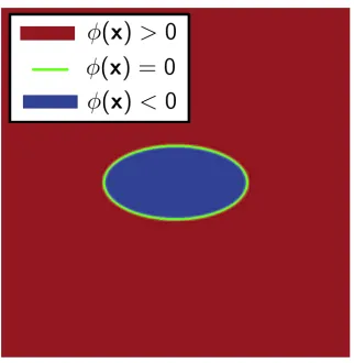
Figure 1. Sign ofφaccording to the position of the interface
Let’s define a bounded domain Ω⊂Rp (p= 2,3) decomposed into two sub-domains Ω
1and Ω2. We denote
Γ the interface between the two partitions. The level set method, as described in [13–15], defines a continuous scalar functionφ(the level set function) in Ω.
• The sub-domains Ω1 and Ω2 and the interface Γ are defined thanks to the level set function (see figure
1) :
Ω1 = {x|φ(x)>0},
Ω2 = {x|φ(x)<0},
Γ = {x|φ(x) = 0}.
• The evolution of the level set is governed by the following advection equation :
∂φ
∂t +u· ∇φ= 0, (1)
It’s known that the advection equation (1) does not conserve the property |∇φ| = 1. To overcome this problem, we use a fast marching method (FMM) when|∇φ|goes far from 1. More precisely, FMM resetsφ as a distance function without moving the interface (see [16] more details). We now introduce the definition of the smoothed delta and Heaviside functions that allow easy computations on the interface Γ without having to explicitly compute the interface
Hε(φ) =
0, φ≤ −ε,
1 2 1 +
φ ε +
sin(πφε ) π
!
, −ε≤φ≤ε,
1, φ≥ε,
δε(φ) =
0, φ≤ −ε,
1 2ε
1 + cos(πφ ε )
, −ε≤φ≤ε,
0, φ≥ε,
where ε is a parameter defining a “numerical thickness” of the interface (a typical value ofε is 1.5 times the mesh size).
Using these two functions allows then to define (e.g. physical) properties having different values in Ω1 and
Ω2. For example we define the viscosities and densities of the inner and outer fluid as follows:
ρφ = ρ2−(ρ2−ρ1)Hε
µφ = µ2−(µ2−µ1)Hε.
As to the integrals over Γ, they are approximated by integrals over the whole domain Ω as follows:
Z Γ 1' Z Ω δε
2.2.
Navier Stokes equations
We consider that both the internal and the external fluids are governed by incompressible Navier Stokes equations :
ρφ ∂u
∂t + (u· ∇)u
− ∇ ·(µφD(u)) +∇p = F in Ω, (2)
∇ ·u = 0 in Ω, (3)
u = g on∂Ω (4)
where u is the velocity of the fluid, pits pressure,D(u) =∇u+ (∇u)T, and F some external force and g a
given function related to the boundary conditions.
A validation of our two-fluid model based on Navier-Stokes equations and the level set advection has been presented in [17] on a bubble simulation benchmark. In this work we also consider the Stokes equations. Indeed, many blood flow applications are in a very low Reynolds number regime. Thus, we use a stationary Stokes model for the fluids
− ∇ ·(µφD(u)) +∇p = F in Ω, (5)
∇ ·u = 0 in Ω, (6)
3.
Vesicles Model
A vesicle is a system of two fluids separated by a membrane. It has been studied by many previous numerical studies, see section1. In this work, we consider a model of membrane with a zero thickness and has three main properties :
• Constant Volume : as both fluids (inside and outside the vesicle) are incompressible and as the membrane is not porous, it results that the total volume (surface in 2D) of the vesicle is constant in time
• Bending Energy : it costs some energy to bend the membrane. This energy has to be taken into account in the model.
• Local Inextensibility : the membrane has to keep the same area (perimeter in 2D) during the simulation time.
We choose to use the model introduced in [6,18] in which the bending energy and the local inextensibility are represented by interfacial forces: the membrane is represented by a force distribution along the interface between inner and outer fluids. In the following section, we briefly describe some details of this model.
3.1.
Bending Force
The bending energy has been introduced by Helfrich in [19] as :
Ec= Z
Γ kB
2 κ
2, (8)
wherekBis the bending modulus of the membrane andκis the local curvature of the interface. By differentiating
the expression (8), Maitreet al [6,18] found the resulting local force. It reads
Fc= Z
Γ kB∇ ·
−κ2
2 n+ 1
|∇φ|(I−n⊗n)∇{|∇φ|κ}
, (9)
whereIstands for the identity tensor andnstands for the normal unit vector to the interface Γ,i.e. |∇∇φφ|. This expression can be then rewritten in the level set formulation by replacing the normal vector by its expression (as a function ofφ) and the integral over Γ by an integral in Ω. Thus, we obtain :
Fc= Z
Ω kB∇ ·
−κ2
2 ∇φ |∇φ|+
1 |∇φ|
I−∇φ⊗ ∇φ |∇φ|2
∇{|∇φ|κ}
δ(φ). (10)
3.2.
Inextensibility Force
In many models, the local area of the vesicle is conserved by adding a Lagrange multiplier which ensures the membrane inextensibility as in [5,17,20,21]. In [22,23], the authors show the possibility to get the quasi inextensibility of the membrane by adding an elastic force using the derivative of an elastic energy. They show that the stretching of the interface is recorded in the gradient modulus ofφ. Indeed, under the assumption that the flow is incompressible, one can write a constitutive law of the stretching related to|∇φ|. The elastic energy reads :
Eel = Z
Ω
E(|∇φ|)δ,
withE(|∇φ|) a constitutive law of the membrane such thatE(1) = 0 (no initial stretching). A simple definition ofE(|∇φ|) is a quadratic law : E(|∇φ|) = Λ
2(|∇φ| −1)
2 so thatE0(∇φ) (the derivative ofE) is a linear law :
it has to be taken large enough to keep almost constant area. By differentiating the energy, it has been shown in [6,22] that one can write the elastic force as :
Fel= Z
Ω
∇E0(|∇φ|)− ∇ ·
E0(|∇φ|) ∇φ |∇φ|
∇φ
|∇φ|
δ(φ). (11)
Using forces to maintain incompressibility has some clear advantages: (i) we can add complexity to the model such as changing the constitutive law of E0 (e.g. a more rigid part which could take into account the cytoskeleton of a red blood cell) or add a new force like a surface tension force, (ii) and the fact that the fluid solver is used as a “black box”: the vesicle model is seen only through the external forcing terms, the density and viscosity which allows for easily changing the fluid solver —e.g. use a non-newtonian model. — However the main drawback is that this technique leads to a larger variation of the surface area than the ones using Lagrange multipliers. Note also that in this model, we need to keep the information of∇φ. Reinitialization is then difficult since it resets |∇φ|= 1 andforgets the stretching information. We explain how to get over this issue in section 4.3. The conservation of the total surface of the vesicle is better than the conservation of the local perimeter since it is enforced by the incompressibility of the fluid. Finally, we just have to add forcing termsFb andFel to equation (2) to simulate the presence of the membrane.
4.
Implementation
4.1.
Discretization
4.1.1. Time Discretization
For stability and accuracy reasons, we choose to use the Crank-Nicolson scheme (CN) to discretize equation (1). It reads
φn+1−φn
∆t + 1 2(u· ∇φ
n+1
+u· ∇φn) = 0. (12)
We could use another scheme like backward differencing scheme of order 2,BDF2, but this method needsφn−2
to computeφnand in this case, at reinitialization step,φchanges roughly and breaks the second order ofBDF2
scheme.
4.1.2. Space Discretization
Both the advection equation (12) and the Stokes equations (5)- (6) are discretized using the finite element method. To do that, we use theC++Finite Element LibraryFeel++[24–26] which allows us to use high order polynomial approximation and work indifferently in 1, 2 or 3 dimensions without changing the code except for the configuration of the problem.
4.1.3. Weak formulation
The problem (1)-(2)-(3) is equivalent to find (u, p, φ) ∈ V ×L20(Ω)×H1(Ω) which verifies ∀(v, q, ψ) ∈ H01(Ω)2×L20(Ω)×H1(Ω) :
ρφ Z
Ω ∂u
∂t + (u· ∇)u
·v+µφ Z
Ω
D(u) :D(v)−
Z
Ω
p∇ ·v =
Z
Ω
(Fc(φ) +Fel(φ))·v, (13)
Z
Ω
q∇ ·u = 0, (14)
u = g on∂Ω, (15)
Z
Ω
∂tφψ+ Z
Ω
(u· ∇φ)ψ+
Z
Ω
S(φ, ψ) = 0, (16)
whereS(φ, ψ) stands for a stabilization term andV ={v∈[H1(Ω)]2|v|
∂Ω=g}.
As to the discretization, we introduce Un+1h , Pn h and Q
m
h the corresponding discrete finite elements spaces
depending on mesh sizehand respectively based on Lagrange polynomials of degreen+ 1,nandm. To handle the fact that the pressure is known up to a constant, we introduce a pseudo compressibility term, p with ≈1e−6, to the Stokes equations.
Let (uh, ph, φh)∈Un+1h ×P n
h×Qmh be the discretization of (u, p, φ). The discrete version of problem
(13)-(14)-(16) becomes : find (uh, ph, φh)∈Un+1h ×P n
h×Qmh which verifies∀(vh, qh, ψh)∈Un+1h ×P n
h×Qmh :
ρφ Z
Ω ∂u
h
∂t + (uh· ∇)uh
·vh+µφ Z
Ω
D(uh) :D(vh)− Z
Ω
ph∇ ·vh = Z
Ω
(Fc(φh) +Fel(φh))·vh,(17)
Z
Ω
qh∇ ·uh+phqh = 0, (18)
uh = g on∂Ω, (19)
Z
Ω
∂tφhψh+ Z
Ω
(uh· ∇φh)ψh+ Z
Ω
S(φh, ψh) = 0. (20)
4.2.
High order derivative
The formulations of bending and elastic forces given by equations (10) and (11) could be problematic when using finite element approximation. Indeed, Fel needs a second order derivative of the level set. Moreover,
recalling that κis of second order derivative, Fc needs some 4th order derivative of φ. Differentiating several
timesφleads to oscillations, especially when low order polynomials are used to approximate it.
In [11] the authors introduced two mixed variables ( ˜ψ=κ|∇φ|and ˜γ=∇|∇φ|) and two new equations to lower the degree of the derivatives. In [10], the authors used an augmented level set (as described in [31]) in which they solve by finite difference schemes an advection equation for φand an other one for∇φ. Moreover, three equations are solved at reinitialization step to take into account the higher derivatives ofφ.
We choose to solve an additional advection equation to calculate the gradient modulus ofφ. Let’s introduce a scalar functione=|∇φ|which verifies
∂te+u· ∇e=−e
∇φ⊗ ∇φ
|∇φ|2 :D(u). (21)
Note that using this equation, we lower the degree of derivative of one.
reinitialize the level set without introducing errors in the calculation of Fel. However, there is still a problem
to achieve 4th order derivative smoothly.
In order to solve this issue, one can do aL2projection of the gradient of any function to derive, which mean,
having a gradient∇f ∈[L2(Ω)]2, findf0∈[L2(Ω)]2 such that∀g∈[L2(Ω)]2
Z
Ω
f0·g=
Z
Ω
∇f·g. (22)
ThisL2projection can lead to oscillations, but we can add a smoothing term proportional to a parameterε s
which has to be small enough so that it does not perturb the accuracy of the projection. This projection leads to the following formulation : find f0∈[H1(Ω)]2, such that ∀g∈[H1(Ω)]2,
Z
Ω
f0·g+εs Z
Ω
∇f0:∇g−εs Z
∂Ω
(∇f0·n)·g=
Z
Ω
∇f·g. (23)
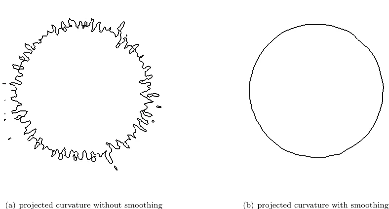
Figure2shows the iso lineκ= 1 whenφ= 0 is a circle of radius 1. One can see that the projected curvature without smoothing (figure2(a)) leads to oscillations, whereas the smoothed curvature (figure2(b)) leads to the expected result.
(a) projected curvature without smoothing (b) projected curvature with smoothing
Figure 2. Iso line 1 of curvature of the level set when the iso lineφ= 0 is a circle of radius 1
4.3.
Reinitialization
When |∇φ| is too different from 1, the support of the Heaviside and Dirac functions (which are defined according toφ) are not symmetric with respect to the interface. Indeed, they are narrowed on the side where
|∇φ|>1 and enlarged on the side where |∇φ| <1. It has been shown in [22] that ˜φ= φ
and δε, we keep the constant size of the interface and avoid the need of very frequent reinitialization. This
projection is called Interface Local Projection (ILP).
Nevertheless, for long time simulation, the gradient of φcan become really high so that, at some point, ˜φ vanishes and creates new artificial interfaces. To overcome this issue, some reinitializations are needed at a low frequency. The method used to reinitializeφis a Fast Marching Method described in [16].
5.
Validation
5.1.
Equilibrium Shape
The first system on which we validate our model is the equilibrium shape of a vesicle in a fluid at rest. Indeed, if we consider a vesicle in a shape which is not the one minimizing its energy, the curvature force makes the membrane move as the fluid around it. This dynamic stops when the vesicle reaches its equilibrium state. In our simulations, we initialize the vesicles as ellipses of perimeterp(which does not correspond to the equilibrium shape).
We solve the Navier-Stokes equations in a rectangular domain containing the vesicle with homogeneous Dirichlet boundary conditions and the external forces modeling the vesicle behavior discussed in the previous section.
To analyze the results of the simulations, we need to define a dimensionless number representing the relative
strength of the involved forces : Rf = R2
0Λ kB
, withR0 = p
2π the radius of a circle having the same area of the vesicle. Note that Rf has to be large enough so that the incompressibility force keeps the perimeter of the
vesicle almost constant. In practice we choose Rf = 5×10⁴ which gives a variation of the total perimeter of
the order of 5% and we use (U2h×P 1 h×Q
1
h) as Finite Element Space approximation.
The parameter which controls the final shape that takes a vesicle is the reduced areaα. It is defined as the
ratio between the area of the vesicle (A) and the area of a disk having the same perimeter, i.e. α= 4πA P2 . It
can be shown that for a reduced area of 1, the shape minimizing the Helfrich energy is a circle. Then decreasing αleads to attain a biconcave shape which is also a characteristic of red blood cells (see figure3(d)). Figure 3 shows our results (blue dots) plotted vs the one obtained in [7] (red line) with a Lattice Boltzmann method. We see a good agreement between the two models. We reported on the graphs the final values of the reduced volume, which has moved from the initial state since we do not conserve exactly the perimeter during all the simulation. This difference in the reduced area can explain the small differences which can be seen between our shapes and the one from [7].
5.2.
“Tank Treading”
5.2.1. Description
The second benchmark that we use to validate our model is the so called tank treading regime. In a shear flow, if the ratio µ2
µ1 between the inner and the outer fluid viscosities is smaller than a certain critical value
(around 5 [32]), the vesicle takes a steady angle with respect to the horizontal axis and the fluid inside the vesicle starts to rotate like a chain of a tank.
Figure4shows a vesicle in a tank treading regime at different times. In this simulation, we setRf = 2×10³.
The simulation was run on 104 elements with a time step ∆t = 3×10⁻³. On figures 4(a), 4(b), membrane forces are not compensating yet the hydrodynamical forces, it is a transient state. From figure4(d) to the end (t= 4.5), the vesicle is at steady state.
5.2.2. Order of approximation
(a)α= 1 (b)α= 0.9
(c)α= 0.8 (d)α= 0.6
Figure 3. Equilibrium shape of vesicles in a fluid at rest for different reduced areas
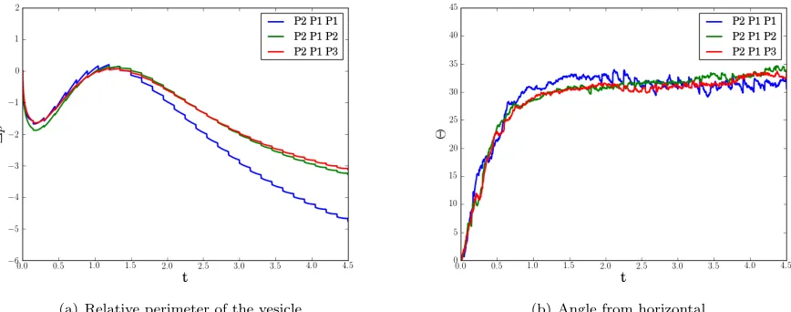
Figure5(a)shows the relative variation of perimeterpof the vesicle ∆p= 100×p−p0 p0
as a function of time for
two different polynomial approximations : U2 h×P
1 h×Q
1 handU
4 h×P
3 h×Q
1
h. The smalljumpsin the perimeter
are due to the reinitializations of level set function.
(a) (b)
(c) (d)
Figure 4. Vesicle in shear flow under tank treading regime.
the vesicle is sheared by the flow and moves to its equilibrium angle. During this time the perimeter increases because the vesicle is stretched. The elastic force increases to minimize the stretching. Finally, the vesicle attains its equilibrium position and one can see that the perimeter decreases because of the error accumulation at steady state. This last effect can be controlled by decreasing the mesh size and/or increasing the polynomial order of the level set approximation.
Moreover, figure 5(b) shows the variation of the angle as a function of time. As we can see on figure 5, increasing the polynomial order of fluid variables approximation doesn’t lead to better results.
At the opposite, figure 6 shows the same tank treading simulation for three sets of approximation spaces (U2
h×P 1 h×Q
1 h), (U
2 h×P
1 h×Q
2
h) and (U 2 h×P
1 h ×Q
3
h) in which the perimeter conservation is improved by
(a) Relative perimeter of the vesicle (b) Angle from horizontal
Figure 5. Vesicle in tank treading regime for two polynomial approximations : U2h×P1h×Q1h
andU4
h×P3h×Q1h
the polynomial order ofφ’s approximation gives a better accuracy in its derivative (up to 4th order) and thus in the forcing terms. The interesting point to retain from fig6(a)is that increasing the order of level set function from 1 to 2 leads to gain a good accuracy (1.5% of the total loss of perimeter in this particular case) and is not too costly in term of computational time (4 times longer than in order 1). At the opposite, increasing the order polynomial of φ from 2 to 3 leads to a small gain in accuracy but the computational time starts to be prohibitive (12 times longer than in order 1). For now we found that U2
h×P 1 h×Q
2
h is a good compromise
between computational time and accuracy.
(a) Relative perimeter of the vesicle (b) Angle from horizontal
Figure 6. Vesicle in tank treading regime for two polynomial approximations : U2h×P 1 h×Q
1 h, U2h×P
1 h×Q
2 handU
2 h×P
1 h×Q
Acknowledgments
Mourad Ismail and Vincent Doyeux acknowledge the financial support from ANR MOSICOB. Vincent Chabannes and Christophe Prud’homme thank the support of the R´egion Rhˆone-Alpes through the project ISLE/CHPID.
Conclusion
We have presented a new finite element implementation of a vesicle model. This model has the advantage to be independent of the fluid solver used since it is expressed only by external forces applied on the interface between inner and outer fluids. We tested this model with a Stokes and a Navier-Stokes fluid. It is possible to add more complexity and use it on a high Reynolds fluid flow or a non Newtonian one. However, this method needs to have a two-fluid interface localized with a good accuracy. To this aim, we developed a level set method in which we do not have to reinitialize too often thanks to the interface local projection. Moreover, when reinitialization is needed we use ILPto initialize a Fast Marching Method. Since the ILPdoesn’t move the position of the interface, we can reinitialize without loss of mass which is usually the main drawback of level set methods. We also described how to handle high order derivative of the level set function without necessarily add as much equations and intermediate variables as the highest derivative degree.
We then validated our model on a first benchmark, the equilibrium shape of a vesicle in a fluid at rest. We compared our results with existing results in literature and found a good agreement. Finally, we reproduced an other behavior of vesicle, the tank treading regime, in which the vesicle takes a steady angle and the membrane rotates around it. We tried different polynomial order approximations to find a good compromise. At the moment increasing only the polynomial approximation of the fluid variables do not lead to significantly better results and we found thatU2h×P
1 h×Q
2
h, for the various configurations we tested, gives the best ratio between
accuracy and computational time. These results have to be confirmed in a near future by rigorous mathematical analysis and new numerical experimentations. Otherwise we need to explore other directions such as perform 3D simulations, handle complex geometries or use more complex fluid models. FEEL++ already allowed us to perform 3D simulations without re-coding the 2D programs.
References
[1] Udo Seifert. Configurations of fluid membranes and vesicles.Advances in Physics, 46(1):13–137, 1997.
[2] M. Mader, V. Vitkova, M. Abkarian, A. Viallat, and T. Podgorski. Dynamics of viscous vesicles in shear flow.The European Physical Journal E: Soft Matter and Biological Physics, 19(4):389–397, 2006-04-01.
[3] G. Coupier, B. Kaoui, T. Podgorski, and C. Misbah. Noninertial lateral migration of vesicles in bounded Poiseuille flow.Physics of Fluids, 20(11):111702–+, November 2008.
[4] Chaouqi Misbah. Vacillating breathing and tumbling of vesicles under shear flow.Phys. Rev. Lett., 96(2):028104, Jan 2006. [5] Badr Kaoui, Alexander Farutin, and Chaouqi Misbah. Vesicles under simple shear flow: Elucidating the role of relevant control
parameters.Phys. Rev. E, 80(6):061905, Dec 2009.
[6] E. Maitre, C. Misbah, P. Peyla, and A. Raoult. Comparison between advected-field and level-set methods in the study of vesicle dynamics.ArXiv e-prints, May 2010.
[7] B. Kaoui, J. Harting, and C. Misbah. Two-dimensional vesicle dynamics under shear flow: Effect of confinement. pre, 83(6):066319–+, June 2011.
[8] Ghigliotti, Giovanni, Selmi, Hassib, Kaoui, Badr, Biros, George, and Misbah, Chaouqi. Dynamics and rheology of highly deflated vesicles.ESAIM: Proc., 28:211–226, 2009.
[9] D. Jamet and C. Misbah. Towards a thermodynamically consistent picture of the phase-field model of vesicles: Local membrane incompressibility.Phys. Rev. E, 76(5):051907, Nov 2007.
[10] D. Salac and M. Miksis. A level set projection model of lipid vesicles in general flows.Journal of Computational Physics, 230(22):8192–8215, September 2011.
[11] Aymen Laadhari.Mod´elisation num´erique de la dynamique des globules rouges par la m´ethode des fonctions de niveau. PhD thesis, Universit´e de Grenoble, 2011.
[14] Ronald Fedkiw Stanley Osher.Level Set Methods and Dynamic Implicit Surfaces. Springer, S.S. Antman, J.E. Marsden, L. Sirovich.
[15] Stanley Osher and James A. Sethian. Fronts propagating with curvature dependent speed: Algorithms based on hamilton-jacobi formulations.Journal of computational physics, 79(1):12–49, 1988.
[16] Christophe Winkelmann. Interior penalty finite element approximation of Navier-Stokes equations and application to free surface flows. PhD thesis, 2007.
[17] V. Doyeux, V. Chabannes, C. Prud’homme, and M. Ismail. Simulation of two fluid flow using a level set method application to bubbles and vesicle dynamics.Journal of Computational and Applied Mathematics, 2012. In Press.
[18] Emmanuel Maitre, Thomas Milcent, Georges-Henri Cottet, Annie Raoult, and Yves Usson. Applications of level set methods in computational biophysics.Mathematical and Computer Modelling, 49(11-12):2161–2169, June 2009.
[19] Ou-Yang Zhong-can and Wolfgang Helfrich. Bending energy of vesicle membranes: General expressions for the first, second, and third variation of the shape energy and applications to spheres and cylinders.Phys. Rev. A, 39(10):5280–5288, May 1989. [20] T. Biben and C. Misbah. Tumbling of vesicles under shear flow within an advected-field approach.Phys Rev E, 67(3):031908–+,
March 2003.
[21] A. Laadhari, C. Misbah, and P. Saramito. On the equilibrium equation for a generalized biological membrane energy by using a shape optimization approach.Physica D: Nonlinear Phenomena, 239(16):1567 – 1572, 2010.
[22] Emmanuel Maitre Georges-Henri Cottet. A level set method for fluid-structure interactions with immersed surfaces. Mathe-matical Models and Methods in Applied Sciences.
[23] Thomas Milcent.Une approche eul´erienne du couplage fluide-structure, analyse math´ematique et applications en biom´ecanique. PhD thesis, Universit´e de Grenoble, 2009.
[24] C. Prud’homme, V. Chabannes, and G. Pena. Feel++: Finite Element Embedded Language in C++. Free Software available at http://www.feelpp.org. Contributions from A. Samake, V. Doyeux, M. Ismail and S. Veys.
[25] Christophe Prud’homme. A domain specific embedded language in C++ for automatic differentiation, projection, integration and variational formulations.Scientific Programming, 14, 2006.
[26] Christophe Prud’homme. Life: Overview of a unified C++ implementation of the finite and spectral element methods in 1d, 2d and 3d. 2007.
[27] Codina Ramon. Comparison of some finite element methods for solving the diffusion-convection-reaction equation.Computer Methods in Applied Mechanics and Engineering, 156(1-4):185–210, April 1998.
[28] G. Hauke. A simple subgrid scale stabilized method for the advection-diffusion-reaction equation.Computer Methods in Applied Mechanics and Engineering, 191(27-28):2925–2947, April 2002.
[29] R.P. Bonet Chaple. Numerical stabilization of vonvection-diffusion-reaction problems. Technical report, 2006.
[30] Erik Burman and Peter Hansbo. Edge stabilization for the generalized stokes problem: A continuous interior penalty method. Computer Methods in Applied Mechanics and Engineering, 195(19-22):2393–2410, April 2006.
[31] Jean-Christophe Nave, Rodolfo Ruben Rosales, and Benjamin Seibold. A gradient-augmented level set method with an opti-mally local, coherent advection scheme.Journal of Computational Physics, 229(10):3802 – 3827, 2010.