F´ed´eration Denis Poisson (Orl´eans-Tours) et E. Tr´elat (UPMC), Editors
A MATRIX-BASED NUMERICAL METHOD FOR THE SIMULATION OF THE
TWO-DIMENSIONAL SINE-GORDON EQUATION
∗,∗∗Francisco de la Hoz
1Abstract. This paper describes a numerical method for the two-dimensional sine-Gordon equation over a rectangular domain using differentiation matrices, in the theoretical frame of matrix differential equations.
R´esum´e. Cette courte note d´ecrit une m´ethode num´erique pour l’´equation de sine-Gordon bidi-mensionnelle sur un domaine rectangulaire en utilisant des matrices de diff´erenciation, dans le cadre th´eorique des ´equations diff´erentielles matricielles.
Introduction
In this paper, we consider the sine-Gordon equation (SGE):
utt(¯x, t) =△u(¯x, t)−sin(u(¯x, t)), u:RN ×R+→R. (1)
This equation is particularly relevant, because it appears in many areas in mathematics, mechanics and the-oretical physics. It describes, for instance, the deformation of a nonlinear crystal-lattice, dislocation in solids, properties of ferromagnets, etc. For many of its applications, see for example [19, pg. 1448], [12, pg. 199], or the introduction of [1], together with their references.
As with other equations, SGE has been most intensively studied for the one-dimensional case. Nevertheless, in the last years, there have appeared a pretty large number of papers devoted to studying numerically the two-dimensional SGE defined over a rectangular domain:
utt(x, y, t) =uxx+uyy−sin(u(x, y, t)), (x, y)∈[−Lx,+Lx]×[−Ly,+Ly], (2)
and imposing almost exclusively homogeneous Neumann boundary conditions ( [3], [4], [21, pg. 134], [11], [17], [18], [10], etc.). Despite using different techniques, the authors do not compare their methods; and their results for the test problems taken from [6] look very similar. On the other hand, in a recently submitted paper [9] (which can be obtained on request), F. de la Hoz and F. Vadillo have developed a pseudo-spectral matrix-based method to solve numerically SGE over an axiparallel rectangular domain in an arbitrary number of spatial dimensions, and with arbitrary time-dependent Neumann boundary conditions. The idea is to discretize the domain at the Chebyshev-Lobatto nodes, approximating the partial derivatives by means of differentiation
∗This work was supported by MEC (Spain), with the project MTM2007-62186, and by the Basque Government, with the project
IT-305-07.
∗∗ I want to thank Fernando Vadillo for his ongoing collaboration on this research area.
1 University of the Basque Country, Department of Applied Mathematics, Plaza de La Casilla 3, 48012 Bilbao (Spain);
e-mail:[email protected]
c
EDP Sciences, SMAI 2012
matrices, and to use a fourth-order Runge-Kutta method with integrating factor [20, chap. 10] to advance in time, avoiding completely the calculation of matrix exponentials and of tensorization.
In this short paper, we announce the main results of [9] for the two dimensional case, i.e., we develop a matrix-based numerical method for the two-dimensional SGE over a rectangular domain with arbitrary Neumann boundary conditions. The structure of the paper is as follows: In Section 1, we formulate the matrix problem; in Section 2, we solve the corresponding linear problem; in Section 3, we develop a first-order numerical scheme with integrating factor; in Section 4, we perform the numerical tests; and, finally, in Section 5, we draw the main conclusions.
1.
Formulation of the matrix problem
Spectral methods have been successfully applied to time-dependent partial differential equations (PDE) and there is an ample literature on this subject (see for instance [14], [2] and [20], as well as the more classic references [15] and [5]). The idea is to approximate the solutionu(x, y, t) by a finite sum:
u(x, y, t)≈U(x, y, t) =
nx
X
k=0
ny
X
l=0
akl(t)φk
x Lx
φl
y Ly
, (3)
where φm(·) = cos(marccos(·)) is the Chebyshev polynomial of degree m; x∈ [−Lx, Lx] and y ∈ [−Ly, Ly].
This approximation is an equality (i.e., a spectral equality) for a large enough number of addends, i.e., a large enough spectrum, except for errors smaller than the accuracy of the machine.
Chebyshev polynomials appear when dealing with non-periodic problems like (2), while, for periodic problems, trigonometric polynomials are the correct choice. There are different approaches to determine the expansion coefficients akl(t): we will focus on pseudo-spectral methods, where akl(t) are required to make the residual
equal zero at as many (suitably chosen) spatial points (xj, yi) as possible. In this case, the natural choice are
the Lobatto-Chebyshev nodes, i.e., (xj, yi) = (Lxcos(jπ/nx), Lycos(iπ/ny)), 0≤j≤nx, 0≤i≤ny.
In our matrix-based philosophy, we do not obtain explicitly the coefficients akl(t). Instead, our evolution
variable is the matrixU(t)∈ M(ny+1)×(nx+1), whereUij(t)≡U(xj, yi, t), 0≤j≤nx, 0≤i≤ny. Notice that we write (xj, yi) rather than (xi, yj), to be coherent withMatlab commands, such asmeshgrid. To discretize
(2), we approximateuxx anduyy by means of the Chebyshev differentiation matrixD[20, chap. 6] [22] [13]:
uyy(xj, yi)≈
1
L2
y
D2
·U, uxx(xj, yi)≈U·
1
L2
x
D2 T
,
whereDT denotes the transpose ofD. Then, (2) becomes
Utt(t) =U(t)·
1
L2
x
D2 T
+
1
L2
y
D2
·U(t)−sin(U(t)), (4)
where the sine is applied pointwise. In the discretization of (2), only the inner elements Uij of the matrix
are considered, i.e., those with 1 ≤ j ≤ nx−1, 1 ≤ i ≤ ny−1. Therefore, we have to recover the border
elements U0j,Unyj,Ui0 andUinx in function of the inner elements ofU by means of the boundary conditions corresponding to (2). More precisely, if ˜U ∈ M(ny−1)×(nx−1) denotes the inner points of U, then it is not difficult [7] to find matricesP1∈ M(ny+1)×(nx−1),P2∈ M(ny−1)×(nx+1) andQ∈ M(ny+1)×(nx+1), such that
Introducing (5) into (4) and restricting ourselves to the inner points, (4) becomes
Utt(t) =A·U(t) +U(t)·BT +C(t)−sin(U(t)), (6)
where, in order not to burden the notation, and without lost of generality, we have omitted the tildes of ˜U. C
is time-independent if the boundary conditions are time-independent, and zero if the boundary conditions are homogeneous. A and B are actually the second-order Chebyshev differentiating matrices with homogeneous Neumann boundary-conditions and applied to the inner nodes; if nx =ny, then L2yA =L2xB. We will solve
numerically (6) and, once calculated its evolution, will recover the border elements ofU(t) from (5).
0 20 40 60 80 100 120 140 −3000
−2500 −2000 −1500 −1000 −500 0
ξ
eigenvalues
0 500 1000 1500 2000
3 4 5 6 7 8 9 10
n
cond(P
A
)
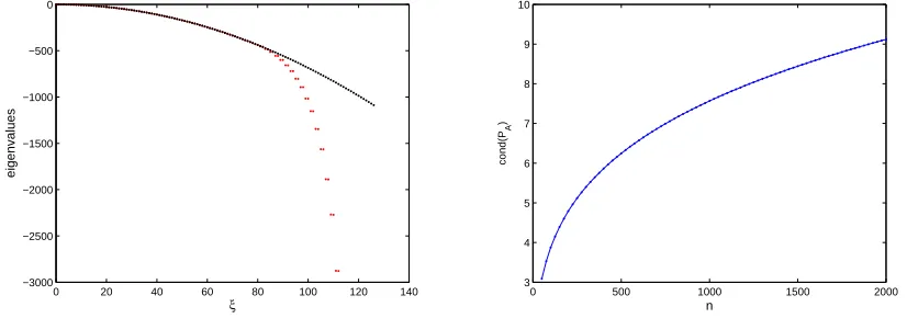
Figure 1. Left: Eigenvalues λξ(A) of the second-order differentiation matrixA with
homo-geneous Neumann boundary conditions, ny = 128, Ly = 6 (red), versus the corresponding
eigenvalues λξ =−(ξπ/2Ly)2 of the continuous problem uxx =λu, ux(−Ly) =ux(+Ly) = 0
(black). Right: Condition number ofPA, as a function of the number of spatial nodesny.
At this point, two crucial observations should be done. The first one is that all the eigenvalues ofA and
B are negative, except for one, which equals zero except maybe for infinitesimal rounding errors. This fact, which is required for stability, is evident from a numerical point of view from the left hand-side of Figure 1. The second crucial observation is the well-conditionedness of the matrices of eigenvectorsPA andPB that appear
in the diagonal decomposition ofAandB, i.e.,DA=P−A1·A·PA andDB=P−B1·B·PB; this is required to
avoid direct calculation of exponential matrices, which is a central idea of this paper. In the right-hand side of Figure 1, we have plotted the 2-norm condition number of the eigenvector matrixPA ofA∈ M(ny−1)×(ny−1), forL= 6, and different ny, being evident that the condition numbers are small and grow sublinearly.
2.
Solving the linear problem
The integrating-factor method is based on the idea that a problem with a linear part plus a nonlinear one can be transformed, so that its linear part is solved exactly (see [20, chap. 10], [8], and their references). Hence, to apply an integrating factor to (6), we need to solve first its linear part
Utt=A·U+U·BT, (7)
Theorem 2.1. Given the time-independent matrices A ∈ M(ny−1)×(ny−1), and B ∈ M(nx−1)×(nx−1), with
diagonal decompositions DA=P
−1
A ·A·PA andDB=P
−1
B ·B·PB, the solution of (7)is
U(t) =PA·
h P−1
A ·U(0)·(P −1
B )T
◦costp−ΛAB
i
·PTB
+PA·
P−1
A ·Ut(0)·(P −1
B )
T
◦p−ΛAB
−1
◦sintp−ΛAB
·PTB V(t) =PA·
h
− P−1
A ·U(0)·(P −1
B )
T
◦p−ΛAB◦sin
tp−ΛAB
i
·PTB
+PA·
h P−1
A ·Ut(0)·(P −1
B )
T
◦costp−ΛAB
i
·PTB,
(8)
where all the operations arepointwise;◦denotes the Hadamard or pointwise product of two matrices [16]; and
ΛAB = [λij]is the matrix whose elements are λij=λi(DA) +λj(DB), for i= 1, . . . , ny−1,j= 1, . . . , nx−1.
Observe that if λij = 0, we take (p−λij)−1sin(tp−λij) ≡ t, so zero eigenvalues cause no concern.
Moreover, since we have proven numerically (left-hand side of Figure 1) that λij ≤0,U(t) and V(t) are real
and bounded∀t >0. On the other hand, if there wereλij >0, there would be stability issues ast→ ∞.
3.
Integrating factor with forward Euler discretization
Let us transform (6) by means of the vec operator [16]:
vec(U) vec(V)
t
=M·
vec(U) vec(V)
+
0
vec(C)−sin(vec(U))
, (9)
whereV=Ut, andMis the block matrix
M=
0 I
B⊕A 0
, (10)
where⊕denotes the Kronecker sum [16], and we have used that vec(A·U(t) +U(t)·BT)≡(B⊕A)·vec(U).
In (9), there is a linear part plus a non-linear part; to get rid of the linear part, we multiply at both sides by the integrating factor exp(−tM), where exp denotes the matrix exponential, getting
exp(−tM)·
vec(U) vec(V)
t
= exp(−tM)·
0
vec(C)−sin(vec(U))
. (11)
Using a forward Euler discretization in time, it becomes
exp(−tn+1M)·
vec(Un+1) vec(Vn+1)
−exp(−tnM)·
vec(Un) vec(Vn)
= ∆texp(−tnM)·
0
vec(Cn)−sin(vec(Un))
. (12)
Multiplying at both sides by exp(tn+1M), we get finally
vec(Un+1) vec(Vn+1)
= exp(∆tM)·
vec(Un) vec(Vn)
+ ∆t
0
vec(Cn)−sin(vec(Un))
which is obviously the solution of (7) at time t = ∆t, with initial data U(0) = Un, and V(0) = Vn +
∆t(vec(Cn)−sin(vec(Un))); hence, by Theorem 2.1,
Un+1=PA·
P−1
A ·Un·(P −1 B )T
◦cos∆tp−ΛAB
+ P−1
A ·[V
n+ ∆t(
Cn−sin(Un))]·(P−1
B )
T
◦p−ΛAB
−1
◦sin∆tp−ΛAB
·PTB,
Vn+1=PA·
− P−1
A ·[V
n+ ∆t(Cn
−sin(Un))]·(P−1
B )
T
◦p−ΛAB◦sin
∆tp−ΛAB
+ P−1
A ·U
n
·(P−1
B )
T
◦cos∆tp−ΛAB
·PTB. (14)
In brief, we have tensorized (6), applied the integrating factor, discretized the equation in time, and destensorized the resulting scheme. The previous ideas can be easily extended to order schemes, by applying a higher-order discretization to (11). In the following section, for comparison’s sake, we have also considered a fourth-order Runge-Kutta discretization of (11).
2 4 6 8 10 12 14
10−4 10−3 10−2 10−1 100 101
−log 2(∆ t)
Error in L
∞−norm at t = 10
First−order scheme in 2D
N = 32 N = 64 N = 128 N = 256 N = 512
2 4 6 8 10 12 14
10−12 10−10
10−8 10−6 10−4 10−2 100 102
−log 2(∆ t)
Error in L
∞−norm at t = 10
Fourth−order scheme in 2D
N = 32 N = 64 N = 128 N = 256 N = 512
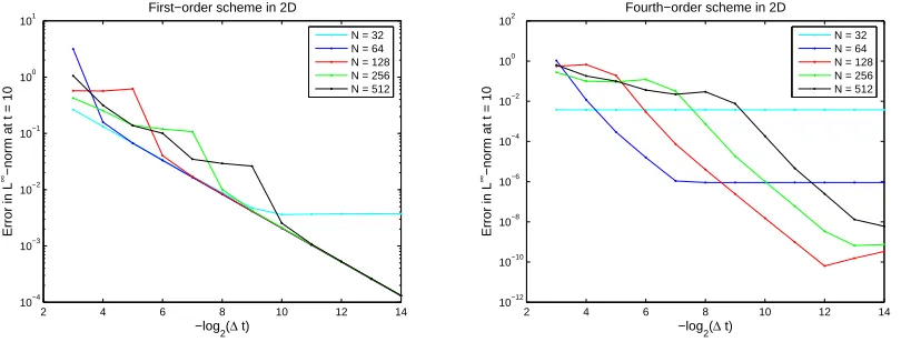
Figure 2. Errors inL∞-norm att= 10, forL
x=Ly = 6, and differentnx=ny =N and ∆t,
corresponding to the first-order scheme (left), and to the fourth-order scheme (right).
4.
Numerical tests
We have considered the theoretical solution of (2),u(x, y, t) = 4 arctan(exp[(√2/2)x+ (√6/2)y−t]), (x, y)∈ [−6,6]2,
∀t≥0; introducing exactly the initial datau(x, y,0) andut(x, y,0), and the inhomogeneous Neumann
boundary conditions ∂xu(±6, y, t), and ∂yu(x,±6, t), ∀t. We have executed the first-order scheme described
above, as well as a fourth-order Runge-Kutta with integrating factor [9], forLx=Ly= 6 and differentnx=ny.
Figure 2 shows the errors obtained inL∞
-norm att= 10, for different ∆t; notice that max(x,y)u(x, y,10)≈5.48. The left-hand side and right-hand side correspond respectively to the first and fourth-order schemes; the orders are evident from the slopes of the (approximately) straight lines that appear: while the first-order may need a prohibitive ∆t to yield good results, the fourth-order method offers a highly remarkable accuracy.
To obtain the highest possible accuracy, a minimum number of nodes N is required. For example, with
N = 32 andN = 64, the minimum possible errors are only about 3.7581·10−3 and 9.0774·10−7, respectively. On the other hand, the method is very stable, even for big N.
the results get slightly worse when we increaseN, they are still very good, even for largeN. For instance, for
N = 512 and ∆t= 2−14, we have an absolute error of about 6.0143
·10−9.
5.
Conclusions
We have developed a new numerical matrix-based method with integrating factor to solve efficiently and accurately the two-dimensional SGE (2), avoiding the explicit calculation of matrix exponentials and the use of Kronecker tensor products. To understand why avoiding tensor products is vital, let be A,B ∈ MN×N,
where all the components of both A and B are positive (so that there are no cancellations); then it can be shown that B⊕A ∈ MN2×N2 has exactly 2N3−N2 non-zero elements, i.e. a sparsity ratio of O(1/N). Therefore, ifN= 511,AandBhave just 261121 elements, versusB⊕A, which has 68184176641 elements, of which 266604541 are nonzero! In other words, the problem becomes quickly intractable. Another virtue of the non-tensor approach is that it can be extended to higher dimensions [9], overcoming the curse of dimensionality. The method can be applied, with little modification, to other types of nonlinear Klein-Gordon equations, with other types of boundary conditions. Furthermore, the techniques of this paper are not necessarily restricted to axiparallel rectangular domains. Indeed, as long as the spatially semi-discretized problem can be written in the form of (6), with eventually another nonlinear term, the general ideas in this paper are applicable.
References
1. E. L. Aero, A. N. Bulygin, and Y. V. Pavlov, Solutions of the three-dimensional sine-Gordon equation, Theoretical and Mathematical Physics158(2009), 313–319.
2. J. P. Boyd,Chebyshev and Fourier Spectral Methods, Dover, 2001.
3. A. G. Bratsos,The solution of the two-dimensional sine-Gordon equation using the method of lines, J. Comput. Appl. Math. 206(2007), 251–277.
4. ,An improved numerical scheme for the sine-Gordon equation in 2+1 dimensions, Int. J. Numer. Meth. Engng75
(2008), 787–799.
5. C. Canuto, M. Y. Hussain, A. Quarteroni, and T. A. Zang,Spectral Methods in Fluid Dynamics, Springer, 1988.
6. P. L. Christiansen and P. S. Lomdahl, Numerical solutions of 2 + 1 dimensional sine-Gordon solitons, Physica 2D (1981), 482–494.
7. F. de la Hoz and F. Vadillo,A Simple Method for Two-Dimensional Advection-Diffusion Equations via Operational Matrices, preprint.
8. ,An integrating factor for nonlinear Dirac equations, Computer Physics Communications181(2010), 1195–1203.
9. ,Numerical simulation of theN-dimensional sine-Gordon equation via operational matrices, Computer Physics
Com-munications183(2012), 864–879.
10. M. Dehghan and A. Ghesmati, Numerical simulation of two-dimensional sine-Gordon solitons via a local weak meshless
technique based on the radial point interpolation method (RPIM), Computer Physics Communications181(2010), 772–786.
11. M. Dehghan and A. Shokri,A numerical method for solution of the two-dimensional sine-Gordon equation using the radial
basis functions, Mathematics and Computers in Simulation79(2008), 700–715.
12. P. G. Drazin and R. S. Johnson,Solitons : an introduction, Cambridge University Press, 1989.
13. E. M. E. Elbarbary and S. M. El-Sayed,Higher order pseudospectral differentiation matrices, Applied Numerical Mathematics 55(2005), no. 4, 425–438.
14. B. Fornberg,A Practical Guide to Pseudospectral Methods, Cambridge University Press, 1998.
15. D. Gottlieb and S. A. Orszag,Numerical Analysis of Spectral Methods: Theory and Applications, SIAM, 1977. 16. N. J. Higham,Function of Matrices. Theory and Computation, SIAM, 2008.
17. D. Mirzaei and M. Dehghan,Boundary element solution of the two-dimensional sine-Gordon equation using continuous linear
elements, Engineering Analysis with Boundary Elements33(2009), 12–24.
18. ,Meshless local Petrov-Galerkin (MLPG) approximation to the two dimensional sine-Gordon equation, J. Comput.
Appl. Math.233(2010), 2737–2754.
19. A. C. Scott, F. Y. F. Chu, and D. W. McLaughlin,The Soliton: A New Concept in Applied Science, Proceedings of the IEEE 61(1973), no. 10, 1443–1483.
20. L. N. Trefethen,Spectral Methods in MATLAB, SIAM, 2000.
21. E. H. Twizell,Computational Methods for Partial Differential Equations, John Wiley & Sons, 1984.