Download Download PDF

(1)

* Corresponding author, Tel: +234-8023278605

COMPUTER

COMPUTER----AIDED ROOT

AIDED ROOT

1 1 1

1, , , , 2222 _{DEPARTMENT OF ELECTRICAL} E

E E

E----mail addresses:mail addresses:mail addresses: mail addresses:1111_{[email protected]}

Abstract Abstract Abstract Abstract

The existing technique of manual calcu The existing technique of manual calcu The existing technique of manual calcu The existing technique of manual calcu studies

studies studies

studies is laborious and time consuming. is laborious and time consuming. is laborious and time consuming. is laborious and time consuming. simple fast mathematical iteration is simple fast mathematical iteration is simple fast mathematical iteration is simple fast mathematical iteration is were formed and te

were formed and te were formed and te

were formed and tested for convergence. A pair of complementary formulas with highest rate of sted for convergence. A pair of complementary formulas with highest rate of sted for convergence. A pair of complementary formulas with highest rate of sted for convergence. A pair of complementary formulas with highest rate of convergence was selected. The process of

convergence was selected. The process of convergence was selected. The process of convergence was selected. The process of were divided into steps which were were divided into steps which were were divided into steps which were were divided into steps which were g

gg

geometric properties of the rooteometric properties of the rooteometric properties of the root----eometric properties of the root de

de de

described in the literature. Rootscribed in the literature. Rootscribed in the literature. Root----loci are drawn to scale instead of rough sketches. scribed in the literature. Rootloci are drawn to scale instead of rough sketches. loci are drawn to scale instead of rough sketches. loci are drawn to scale instead of rough sketches.

Keywords: Keywords: Keywords:

Keywords: control system, stability, transient response,

1. 1. 1.

1. IntroductionIntroductionIntroductionIntroduction

A control system is the means by which any parameter of interest in a machine, mechanism or equipment is maintained or altered in accordance with desired manner. Introduction of feedback into a control system has the advantages of reducing sensitivity of system performance to internal variations in system parameters, improving transient response and minimizing the effects of disturbance signals. However, feedback increases the number of components, increases complexity, reduces gain and introduces the possibility of instability [1 – 6].

A system is stable if its response to a bounded input vanishes as time t approaches

unstable system cannot perform any

A stable system with low damping is also not desirable. Therefore, a stable system must also meet the specifications on relative stability which is a quantitative measure of how fast the transients die out with time in the system. The location of roots of system’s characteristic equation determines the stability of the system -5, 7, 8]. The roots of the system’s characteristic equation are the same as the poles of the closed loop system.

Ideally, a desired performance can be achieved by a control system by adjusting the location of its roots in the s-plane by varying one or more system parameters. Root-locus Method is a linear

8023278605

AIDED ROOT

AIDED ROOT----LOCUS NUMERICAL TECHNIQUE

LOCUS NUMERICAL TECHNIQUE

A. R. Zubair A. R. ZubairA. R. Zubair

A. R. Zubair1,1,1,1,* * * * _{,,,, A. Olatunbosun}_{A. Olatunbosun}_{A. Olatunbosun}_{A. Olatunbosun}2222

LECTRICAL/ELECTRONIC ENGINEERING, UNIVERSITY OF IBADAN

[email protected], 2222_{[email protected]}

The existing technique of manual calcu The existing technique of manual calcu The existing technique of manual calcu

The existing technique of manual calculation and plotting of rootlation and plotting of rootlation and plotting of rootlation and plotting of root----locuslocuslocuslocus of a control system for stability of a control system for stability of a control system for stability of a control system for stability is laborious and time consuming.

is laborious and time consuming. is laborious and time consuming.

is laborious and time consuming. A computerA computerA computerA computer----aided rootaided rootaided root----locus numerical technique based on aided rootlocus numerical technique based on locus numerical technique based on locus numerical technique based on simple fast mathematical iteration is

simple fast mathematical iteration is simple fast mathematical iteration is

simple fast mathematical iteration is developed to eliminate this developed to eliminate this developed to eliminate this rigourdeveloped to eliminate this rigourrigourrigour. Alternative iteration formulas . Alternative iteration formulas . Alternative iteration formulas . Alternative iteration formulas sted for convergence. A pair of complementary formulas with highest rate of sted for convergence. A pair of complementary formulas with highest rate of sted for convergence. A pair of complementary formulas with highest rate of sted for convergence. A pair of complementary formulas with highest rate of convergence was selected. The process of

convergence was selected. The process of convergence was selected. The process of

convergence was selected. The process of automatic automatic automatic determination of rooautomatic determination of roodetermination of roots and plotting of rootdetermination of roots and plotting of rootts and plotting of rootts and plotting of root were divided into steps which were

were divided into steps which were were divided into steps which were

were divided into steps which were analyzedanalyzedanalyzedanalyzed, simplified and coded into computer, simplified and coded into computer, simplified and coded into computer, simplified and coded into computer

----loci obtained with this technique are found to conform to those loci obtained with this technique are found to conform to those loci obtained with this technique are found to conform to those loci obtained with this technique are found to conform to those loci are drawn to scale instead of rough sketches.

loci are drawn to scale instead of rough sketches. loci are drawn to scale instead of rough sketches. loci are drawn to scale instead of rough sketches.

control system, stability, transient response, root-locus, iteration

A control system is the means by which any of interest in a machine, mechanism or equipment is maintained or altered in accordance Introduction of feedback into a control system has the advantages of of system performance to internal variations in system parameters, improving transient response and minimizing the effects of disturbance signals. However, feedback ncreases the number of components, increases complexity, reduces gain and introduces the

A system is stable if its response to a bounded input vanishes as time t approaches ∞. An any control task. A stable system with low damping is also not desirable. Therefore, a stable system must also meet the specifications on relative stability which is a quantitative measure of how fast the in the system. The oots of system’s characteristic equation determines the stability of the system [1 The roots of the system’s characteristic equation are the same as the poles of the

closed-desired performance can be achieved by by adjusting the location of its plane by varying one or more locus Method is a linear

time invariant control system design techniqu that determines the roots of the characteristic equation (or closed-loop po

loop gain-constant K is increased from zero to infinity [9, 10]. The root

complete dynamic response of the system and is a measure of the sensitivity of the roots to variation in the parameter (open

constant K) [11]. It yields frequency response of the system and can also be used to solve problems in the time domain. The basic task in root-locus technique is to determine the closed loop pole configuration from the configuration of the open-loop poles and zeros.

The locus of the roots or closed

plotted in the s-plane. This is a complex plane, since s=

σ

+ j

ω

. The real part,

the exponential term of the time response, and if positive will make the system unstable. Any locus in the right-hand side of the plane therefore represents an unstable system. The imaginary part,

ω

, is the frequency of transient oscillation. When a locus crosses the imaginary axis,

the control system is on the verge of instability; where transient oscillations neither increase, nor decay, but remain at a constant value. The design method requires the closed

plotted in the s-plane as K is varied from zero to infinity, and then a value of K selected to provide the necessary transient response as required by

Nigerian Journal of Technology (NIJOTECH)

Vol. 33. No. 1.

http://dx.doi.org/10.4314/njt.v33i1.

LOCUS NUMERICAL TECHNIQUE

BADAN, NIGERIA

[email protected]

of a control system for stability of a control system for stability of a control system for stability of a control system for stability locus numerical technique based on locus numerical technique based on locus numerical technique based on locus numerical technique based on . Alternative iteration formulas . Alternative iteration formulas . Alternative iteration formulas . Alternative iteration formulas sted for convergence. A pair of complementary formulas with highest rate of sted for convergence. A pair of complementary formulas with highest rate of sted for convergence. A pair of complementary formulas with highest rate of sted for convergence. A pair of complementary formulas with highest rate of

ts and plotting of root ts and plotting of root ts and plotting of root ts and plotting of root----locus locus locus locus , simplified and coded into computer

, simplified and coded into computer, simplified and coded into computer

, simplified and coded into computer programs. The programs. The programs. The programs. The loci obtained with this technique are found to conform to those loci obtained with this technique are found to conform to those loci obtained with this technique are found to conform to those loci obtained with this technique are found to conform to those loci are drawn to scale instead of rough sketches.

loci are drawn to scale instead of rough sketches. loci are drawn to scale instead of rough sketches. loci are drawn to scale instead of rough sketches.

time invariant control system design technique that determines the roots of the characteristic loop poles) when the open-constant K is increased from zero to

. The root-locus shows the complete dynamic response of the system and is a measure of the sensitivity of the roots to variation in the parameter (open-loop

gain-. It yields frequency response of the system and can also be used to solve problems in the time domain. The basic task in locus technique is to determine the closed-loop pole configuration from the configuration of

loop poles and zeros.

The locus of the roots or closed-loop poles are plane. This is a complex plane, The real part,

σ

, is the index in the exponential term of the time response, and if ystem unstable. Any locus hand side of the plane therefore represents an unstable system. The imaginary , is the frequency of transient oscillation. When a locus crosses the imaginary axis,

σ

=0, he control system is on the verge of instability; where transient oscillations neither increase, nor decay, but remain at a constant value. The design method requires the closed-loop poles to be plane as K is varied from zero to and then a value of K selected to provide the necessary transient response as required by

Nigerian Journal of Technology (NIJOTECH)

www.nijotech.com

http://dx.doi.org/10.4314/njt.v33i1.9

(2)

Nigerian Journal of Technology, Nigerian Journal of Technology, Nigerian Journal of Technology,

Nigerian Journal of Technology, Vol. 33, No. 1, January 2014 Vol. 33, No. 1, January 2014 Vol. 33, No. 1, January 2014 Vol. 33, No. 1, January 2014

61

the performance specification. The loci always commence at open-loop poles (denoted by x) and terminate at open-loop zeros (denoted by o) when they exist [1 – 5, 9, 10, 12].

In the literature, there exist eight rules based on elementary geometric properties of root-locus which lead to rough sketch of root locus. These rules govern the important features of the root-locus method such as asymptotes, roots condition on the real axis, breakaway points, and imaginary axis crossover [13 – 16]. These rules or steps involve some calculations but avoid determination of actual roots. There are other approaches which use complex analytic or semi-analytic representation that involve the use of equations of the loci [14, 17 – 25]. There is also a computer aided root-locus method based on complex conversion of solution of a parameterized family of algebraic problems into solution of a set of associated differential equations [12]. In this paper, a computer-aided root-locus numerical technique is developed based on simple and fast mathematical iteration.

2.0 2.0 2.0

2.0 RootRootRootRoot----Locus Locus Locus Locus Numerical TechniqueNumerical TechniqueNumerical TechniqueNumerical Technique

Figure 1 shows a closed-loop system with negative feedback; G(s) is the forward-part gain. H(s) is the feedback gain. The transfer function of the system is given by Eqn (1) [1 - 5]. The denominator of the transfer function set to zero is referred to as the characteristic equation:

0 ) ( ) (

1+G s H s = .

Figure 1: Closed-Loop System with Negative Feedback ) ( ) ( 1 ) ( ) ( ) ( s H s G s G s R s C + = (1)

The open-loop transfer function is given as in Eqn. (2). )] ( )][ 1 ( )]...[ 2 ( )][ 1 ( [ )] ( )][ 1 ( )]...[ 2 ( )][ 1 ( [ ) ( ) ( n p s n p s p s p s m z s m z s z s z s K A B K s H s G − − − − − − − − − − = = (2)

z(1), z(2), z(3), …, z(m-1) and z(m) are m open-loop zeros and p(1), p(2), p(3), …, p(n-1) and p(n) are n open-loop poles. Given the open-loop poles and zeros, the task is to deduce the configuration of the closed-loop poles as K varies

from zero to infinity. The characteristic equation becomes: 0 KB A ; 0

1+ = + =

A B

K (3)

The root-locus technique presented in this paper is divided into four steps.

2.1 2.12.1

2.1 Step 1Step 1Step 1Step 1:::: Expansion for the Formation of Expansion for the Formation of Expansion for the Formation of Expansion for the Formation of Characteristic Equation

Characteristic Equation Characteristic Equation Characteristic Equation

The first step is the formation of polynomials A and B from the given open-loop poles and zeros respectively. This step involves expansion. A and B are given as

)

1 (

)

2 (

)

3 (

...

)

(

1)s

a(n

)]

(

)][

1 (

[

)]...

3 (

)][

2 (

)][

1 (

[

2 1

a

s

a

s

a

s

n

a

n

p

s

n

p

s

p

s

p

s

p

s

A

n n

+

=

−

=

− and ) 1 ( ) 2 ( ) 3 ( ... ) ( 1)s b(m )] ( )][ 1 ( [ )]... 3 ( )][ 2 ( )][ 1 ( [ 2 1 b s b s b s m b m z s m z s z s z s z s B m m + + + + + + = − − − − − − = −

Suppose an Nth _order _polynomial

) 1 ( ) 2 ( ... ) ( ) 1 ( ) ( 1 c s c s N c s N c s

C N N

+ + + + + = − is multiplied with (s−r) where r is a real open-loop pole or zero. The product is a (N+1)th_order polynomial ) 1 ( ) 2 ( ... ) ( ) 1 ( ) 2 ( )

(_s _d _N _s 1 _d _N _s _d _N _s 1 _d _s _d

D ₌ ₊ N+ ₊ ₊ N₊ N− ₊ ₊ ₊

such that      = − + = − − + = − = 1 for y ) ( 1) (N to 2 for y ) ( ) 1 ( 2) N ( for y ) 1 ( d(y) y rc y rc y c y c (4)

) 1 ( ) 2 ( ... ) ( ) 1 ( )

(_s _c _N _s _c _N _s 1 _c _s _c

C ₌ ₊ N₊ N− ₊ ₊ ₊

is multiplied with [s−(r+ jh)][s−(r− jh)] where (r+jh) and (r-jh) are complex conjugate open-loop poles or zeros. The product is a (N+2)th

order polynomial

) 1 ( ) 2 ( ... ) 1 ( ) 2 ( ) 3 ( )

( 2 1

d s d s N d s N d s N d s D N N N + + + + + + + + = + + such that:         = = + − + = + − + − + = − + − + = − = 1 for y ) ( ) 1 ( 2 for y ) ( ) 1 ( ) 1 ( ) 2 ( 1) (N to 3 for y ) ( ) 1 ( ) 1 ( ) 2 ( ) 2 ( t(3) 2) N ( for y ) 1 ( ) 2 ( ) 2 ( t(3) 3) N ( for y ) 2 ( t(3) ) ( y c t y c t y c t y c t y c t y c y c t y c y c y d (5) where ) 1 ( ) 2 ( ) 3 ( )] ( )][ (

[_s₋ _r₊ _jh _s₋ _r₋ _jh ₌_t _s2₊_t _s₊_t 2 2 ) 1 ( ; 2 ) 2 ( ; 1 ) 3

( t r t r h

(3)

62

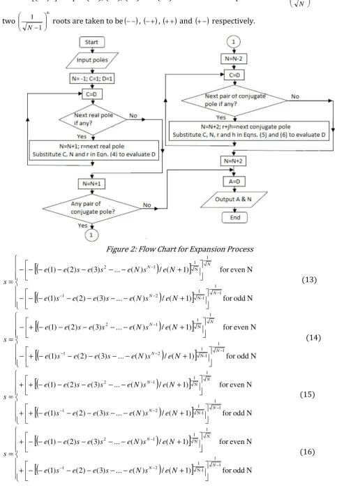
Eqns. (4) and (5) give the general models for expansion involving a single real pole or zero and a pair of conjugate complex pole or zero respectively. As illustrated with the flow chart of Figure 2, the expansion of A starts with C(s)=1 (order zero) multiplied with s−r for the first real pole. The product D obtained is feedback to the multiplication process as C and the process is repeated for other real poles. The new product D is feedback as C which is multiplied with

) 1 ( ) 2 ( ) 3 ( )] ( )][ ( [ 2 t s t s t jh r s jh r

s− + − − = + + for the

first pair of conjugate poles. The process is repeated for other pairs of conjugate poles. A is set equal to the final product D. The whole process is repeated for B using zeros instead of poles. With the substitution of A, B and a value for K, the characteristic Eqn. (3) is given as in Eqn. (7). The characteristic equation is said to be of order N and has N roots.

0 ) 1 ( ) 2 ( ) 3 ( ... ) ( 1)s (N ) ( 2 1 = + + + + + + = − e s e s e s N e e s

E N N

(7)

2.2 Step 2: Determination of Roots for a 2.2 Step 2: Determination of Roots for a 2.2 Step 2: Determination of Roots for a

2.2 Step 2: Determination of Roots for a Value Value Value Value of Kof Kof Kof K Having obtained the characteristic equation, the next step is to determine the roots for a value of K. This step is classified into three sub-steps.

2.2.1 Sub-Step 2.1: Iteration For N=1, the root is:

) 2 ( ) 1 ( e e

r =− (8)

For N=2, one of the roots is

) 3 ( 2 ) 3 ( ) 1 ( 4 ) 2 ( ) 2 ( 2 e e e e e

r= − − − (9)

For N>2, a root of the characteristic Eqn. (7) is obtainable by iterative technique. Iteration computes a sequence of progressively accurate iterates to approximate the solution of an equation [26,27]. Iteration formula is obtainable from Eqn. (7) by making s the subject of formula. Retaining the term e(2)s in Eqn. (7) on the left hand side (LHS), moving all other terms to the right hand side (RHS) and dividing both sides by e(2) lead to the iteration formula of Eqn. (10).

) 2 ( / ) 1 ( ) ( ... ) 4 ( ) 3 ( ) 1 ( 1 3 2 e s N e s N e s e s e e s N N       + − − − − − − = − (10)

Retaining the term e(N+1)sN_{in Eqn. (7) on LHS,} moving all other terms to RHS, dividing both sides by e(N+1) and evaluating

th 1      

N root of both sides lead to the even version of the iterative formula of Eqn. (11). This is used if N is even. Retaining the term e(N+1)sN_{in Eqn. (7) on LHS,} moving all other terms to RHS, dividing both sides by e(N+1)s and evaluating

th 1 1       −

N root of both sides lead to the odd version of the iterative formula of Eqn. (11). This is used if N is odd (N-1 is even). Eqns. (11) and (12) are the same except that the result of

th 1      

N root and

th 1 1       −

N root are

taken to be positive in Eqn. (11) but negative in Eqn. (12). For example, the result of 16¼_{is either} +2 or -2.

(

)

[

]

(

)

[

]

     + − − − − − + + − − − − − + = − − − N odd for ) 1 ( / ) ( ... ) 3 ( ) 2 ( ) 1 ( N even for ) 1 ( / ) ( ... ) 3 ( ) 2 ( ) 1 ( 1 -N 1 2 1 N 1 1 2 N e s N e s e e s e N e s N e s e s e e s N N (11)

(

)

[

]

(

)

[

]

     + − − − − − − + − − − − − − = − − − N odd for ) 1 ( / ) ( ... ) 3 ( ) 2 ( ) 1 ( N even for ) 1 ( / ) ( ... ) 3 ( ) 2 ( ) 1 ( 1 -N 1 2 1 N 1 1 2 N e s N e s e e s e N e s N e s e s e e s N N (12)

Eqns. (13) to (16) are obtainable from Eqn. (11) by breaking down the

th 1      

N root into two

th 1       N

roots or breaking down the

th 1 1       −

N root into two

th 1 1       −

N roots on the RHS. For example +16

(4)

63

same as [(16)½_]½_{. Eqns. (13), (14), (15) and (16) are the same except that the two}

th 1      

N roots or the two th 1 1       −

N roots are taken to be

(

−−

)

,

(

−+

)

,

(

++

)

and

(

+−

)

respectively.

Figure 2: Flow Chart for Expansion Process

(

)

[

]

(

)

[

]

              + − − − − − − −       + − − − − − − − = − − − − N odd for ) 1 ( / ) ( ... ) 3 ( ) 2 ( ) 1 ( N even for ) 1 ( / ) ( ... ) 3 ( ) 2 ( ) 1 ( 1 1 1 -N 1 2 1 1 N 1 1 2 N N N N N e s N e s e e s e N e s N e s e s e e

s (13)

(

)

[

]

(

)

[

]

              + − − − − − + −       + − − − − − + − = − − − − N odd for ) 1 ( / ) ( ... ) 3 ( ) 2 ( ) 1 ( N even for ) 1 ( / ) ( ... ) 3 ( ) 2 ( ) 1 ( 1 1 1 -N 1 2 1 1 N 1 1 2 N N N N N e s N e s e e s e N e s N e s e s e e

s (14)

(

)

[

]

(

)

[

]

              + − − − − − + +       + − − − − − + + = − − − − N odd for ) 1 ( / ) ( ... ) 3 ( ) 2 ( ) 1 ( N even for ) 1 ( / ) ( ... ) 3 ( ) 2 ( ) 1 ( 1 1 1 -N 1 2 1 1 N 1 1 2 N N N N N e s N e s e e s e N e s N e s e s e e

s (15)

(

)

[

]

(

)

[

]

              + − − − − − − +       + − − − − − − + = − − − − N odd for ) 1 ( / ) ( ... ) 3 ( ) 2 ( ) 1 ( N even for ) 1 ( / ) ( ... ) 3 ( ) 2 ( ) 1 ( 1 1 1 -N 1 2 1 1 N 1 1 2 N N N N N e s N e s e e s e N e s N e s e s e e

(5)

64

The alternative iteration formulas Eqns. (10) to (16) were subjected to tests to determine the most reliable or effective. The results and conclusion of the tests are presented and discussed in section 3.1. A guess value of s is substituted in the right side of the iteration formula; a new value of s is computed and substituted back in the right side of the iteration formula and the process is repeated T times. s will converge to a root r of the characteristic equation. The higher the T, the closer the result of iteration to the root and the more time the process takes. Therefore T should not be too small and should not be too large. In some cases, s may not converge to the root [26, 27]. There is need to validate the result obtained as a root.

2.2.2 Sub-Step 2.2: Root Validation Test

The final value of s (s=r) obtained by iteration is tested by substituting the value of s in the test equation, Eqn. (17) which is adapted from the characteristic equation Eqn. (7). rvt is computed. If rvt is equal to 0 or less than 0.00004, s is accepted and recorded as a root; otherwise it is rejected.

) 1 ( ) 2 ( ) 3 ( ... ) ( 1)s

(N _e _N _s 1 _e _s2 _e _s _e

e

rvt₌ ₊ N₊ N− ₊ ₊ ₊ ₊

(17)

2.2.3 Sub-Step 2.3: Grouping of Accepted Root into a Sub-branch of Root-Locus

Accepted root is plotted as a standalone dot (.) on a root-locus dots-plot. Root-locus for a system with n open-loop poles has n branches. A branch of root-locus starts at an open loop pole usually marked with ‘x’ and ends at an open loop zero usually marked with ‘o’ or at infinity. At breakaway points, each single branch breaks into sub-branches. For the purpose of joining the dots with a curve, each accepted root is checked and grouped into a sub-branch of the root-locus. Based on the root-locus dots-plot generated by the algorithm, a number of computer program conditional statements guide the placement of the accepted root into the right sub-branch. An example is presented section 3.3 and illustrated in figure 5.

2.2.4 Sub-Step 2.4: Division Process for Next Root Having obtained a root, whether the root is acceptable or not in Sub-Step 2.2, there is need to divide Eqn. (7) to obtain a lower order characteristic equation for the next root. For a real root r, Eqn. (7) is divided by (s−r) and the order is reduced by 1. A complex root r=σ+ jω

predicts it’s conjugate, r=σ− jω, and vice versa. Therefore, for a complex root r, Eqn. (7) is divided by (s−σ+ jω)(s−σ− jω) and the order is reduced by 2.

) 1 ( ) 2 ( ... ) 1 ( ) ( )) 1 ( )

( 1 2

e s e s

N e s N e s N e s

E N N N

+ + + − + +

+

= − −

is divided by s−r where r is a real root. The quotient a (N-1)th _order _polynomial

) 1 ( ) 2 ( ...

) 2 ( )

1 ( )

( )

( 1 2 3

d s d

s N d s

N d s N d s

D N N N

+ +

+ −

+

= − − −

such that

  

= +

+ +

= +

=

1 to 1) -N ( for y ) 1 ( ) 1 (

N for y ) 1 ( ) (

y rd y

e y e y

d (18)

Suppose a Nth _order _polynomial

) 1 ( ) 2 ( ... ) 1 ( ) ( )) 1 ( )

( 1 2

e s e s

N e s N e s N e s

E ₌ ₊ N₊ N− ₊ ₋ N− ₊ ₊ ₊

is divided by a pair of conjugate roots, )

)(

(s−σ+ jω s−σ − jω . The quotient is a (N-2)th order polynomial :

) 1 ( ) 2 ( ... )

3 (

) 2 ( )

1 ( ) (

4

3 2

d s d s

N d

s N d s

N d s D

N

N N

+ +

+ −

+

− + −

=

−

− −

such

that

    

= +

− + − +

= +

− +

= +

=

1 to 3) -N ( for y ) 2 ( ) 1 ( ) 2 (

2 -N for y ) 1 ( ) 2 (

1 -N for y ) 2 ( ) (

y pd y

td y

e

y td y

e y e y d

(19) where

p ts s j s j

s− + − − = 2+ +

) )(

( σ ω σ ω ;

2 2

;

2σ =σ +ω −

= p

t (20)

Eqns. (18) and (19) give the general models for the division process involving a single real root and a pair of conjugate complex root respectively.

2.2.5 Repetition of Sub-Steps 2.1 to 2.4 for Next Root

The output D of the division process (Sub-Step 2.4) is feedback as E (characteristic equation) to the iteration process (Sub-Step 2.1) which is repeated to obtain the next root. The next root is subjected to validation test (Sub-Step 2.2); if it is a valid root, it is plotted as a standalone dot (.) on root-locus dots-plot and it is grouped into a sub-branch (Sub-Step 2.3). Sub-Step 2.4 is also repeated to update D. The sub-steps 2.1, 2.2, 2.3 and 2.4 are repeated until all the N roots have been obtained and the polynomial D is reduced to

1 ) (s =

D .

2.3 2.3 2.3

2.3 Step 3: Plotting of RootStep 3: Plotting of RootStep 3: Plotting of Root----LocStep 3: Plotting of RootLocLocLocusususus

(6)

65

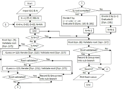
of K are determined as explained in Step 2. Figure 3 shows the flow chart for the determination and plotting of the root-locus.

2.4 Adding Details to th 2.4 Adding Details to th 2.4 Adding Details to th

2.4 Adding Details to the Roote Roote Roote Root----LocusLocusLocusLocus

Having plotted the root-locus, the asymptotes, breakaway points and imaginary axis crossover can be added. For large values of K, root-locus branches are parallel to lines called asymptotes. There are (n-m) asymptotes [1 - 5]. Point of intersection of asymptotes on the real axis is given as in Eqn. (21) [1 - 5].

) (

zeros) loop -open of part (real poles) loop -open of part (real

m n Pasx

− −

=

∑

(21) The angles between asymptotes and the real axis are given as in Eqn. (22) [1 - 5].

) 1 (

..., , 2 , 1 , 0 where )

( ) 1 2 ( )

( = − −

− +

= q n m

m n

q

q π

θ (22)

Breakaway points are obtained as the solution of 0

= ds dK

[1 - 5]. But 1+ =0

A B

K ,

Therefore,

0 )

(

2 =

+ − = − =

B ds dB A ds dA B

ds B A d ds dK

. .i.e − + =0

ds dB A ds dA

B (23)

Eqn. (23) is solved for the breakaway points as illustrated in Figure 4.

The points of intersection of the root-locus with the imaginary axis are called imaginary axis crossover. At these points, the system is said to be marginally stable. Routh-Hurwitz stabilty criterion is used to obtain value(s) of K for marginal stability. Roots of the characteristic equation corresponding to these values of K include the imaginary axis crossover points. The various steps and sub-steps are coded into computer programs. The required inputs to these programs are the open-loop poles and zeros and the output is the root-locus.

3. Tests and Results 3. Tests and Results 3. Tests and Results 3. Tests and Results

3.1 Convergence of Alternative Iteration Formula 3.1 Convergence of Alternative Iteration Formula 3.1 Convergence of Alternative Iteration Formula 3.1 Convergence of Alternative Iteration Formulassss The alternative iteration formulas Eqns. (10) to (16) discussed in Sub-Step 2.1 are tested with an open-loop transfer function. For each iteration formula, the number of successful iterations which produced valid roots and number of failed iterations which produced non-valid roots are recorded and presented in Table 1. Percentage success which is the ratio of successful iterations

to total iterations expressed in percentage for each formula is also listed in Table 1. Eqns. (12) and (14) are found to be similar and displayed the same performance. Eqn. (12) is found to be most successful with 83.41% success followed by Eqn. (13) with 14.29% success.

In another experiment, Eqns. (12) and (13) were used complementarily such that Eqn. (12) is used normally and Eqn. (13) is only used when Eqn. (12) failed to produce valid root. 97.27% success was achieved as listed in Table 1. It is therefore concluded that complementary use of iteration formulas Eqns. (12) and (13), is the choice for best performance.

The flowchart of Figure 3 is actually based on complementary use of Eqns. (12) and (13) as iteration formulas.

The effect of use of versions of iteration formulas for even and odd N are tested for two different open-loop transfer functions and the results are summarised in Table 2. Complementary use of both versions produced the best results. It is therefore concluded that, when N is odd, version for odd N should be used and when N is even, version for even N should be used.

Figure 4: Flow Chart for the Determination of Breakaway Points.

3.2 Sample Root 3.2 Sample Root3.2 Sample Root

3.2 Sample Root----Locus Plots Locus Plots Locus Plots Locus Plots

Sample root-loci plots for a number of systems are obtained with this computer-aided root-locus numerical technique. These plots are presented in Table 3.

3.3 Adding Details to the Root 3.3 Adding Details to the Root3.3 Adding Details to the Root

3.3 Adding Details to the Root----Locus PlotLocus PlotLocus PlotLocus Plot

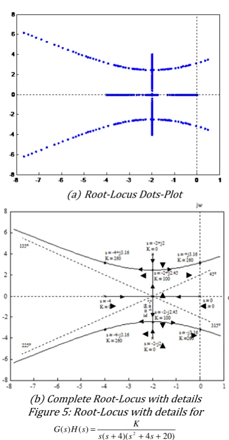
The root-locus dots-plot obtained for a system

with open-loop transfer function

) 20 4 )( 4 ( ) ( )

( ₂

+ + + =

s s s s

K s

H s

G is shown in Figure

5(a). The details for this system are obtained and are presented in Figure 5(b) and Table 4.

Start

Obtain A & B as in Step 1 Differentiate A & B

Obtain the products

ds dA B and

ds dB A (step 1)

Assemble Eqn. (23)

Obtain roots of Eqn. 23 Step 2.1, 2.2 & 2.4 Substitute each root in Eqn. (3) to obtain values of K corresponding to the breakaway points

(7)

66

It is not necessary to find these details before plotting the root-locus. However if values of K for breakaway points are determined first, it will assist the choice of intervals in the values of K to be used. For this open-transfer function, K is varied from 0 to 62 at incremental interval of 2. K is varied from 63.5 to 64.5 at the incremental interval of 0.05. K is varied from 66 to 98 at the

incremental interval of 2. K is varied from 99.5 to 100.5 at the incremental interval of 0.05. Finally K is varied from 102 to 5000 with varying incremental interval 2 (initially) to 100 (later) and then finally 500. K must vary very slowly near breakaway points.

Figure 3: Flow Chart for the Determination and Plotting of Root-Locus as K Varies from 0 to ∞

Table 1: Convergence of Alternative Iteration Formulas for open-loop transfer function

) 20 4 )( 4 ( ) ( )

( ₂

+ + + =

s s s s

K s

H s G

Equation

No of successful

iterations

No of failed iterations

%

success Remark

(10) 0 868 0% not reliable

(12) 724 144 83.41% most reliable

(13) 124 744 14.29% reliable near break away point

(14) 724 144 83.41% same as Eqn. (12)

(16) 16 852 1.84% not reliable

(12) & (13) 844 24 97.27% Eqn. (13) is used when Eqn. (12) fails

(8)

67

Table 2: Convergence of Even and Odd Versions of Alternative Iteration Formulas

Equation No of successful iterations

No of failed iterations

% success Remark

) 20 4 )( 4 ( ) ( )

( ₂

+ + + =

s s s s

K s

H s G

(12) & (13) even version only

595 273 68.55% Only version for even N was used for both even and odd N

(12) & (13) odd version only

0 868 0% Only version for odd N was used for both even and odd N

(12) & (13) both versions

844 24 97.27% Both versions were used as appropriate

) 13 4 )( 4 )( 2 (

) 2 2 )( 3 )( 1 ( ) ( )

( ₂

2

+ + + +

+ + + + =

s s s s s

s s s s K s H s G

(12) & (13) even version only

1 1088 0.0009% Only version for even N was used for both even and odd N

(12) & (13) odd version only

185 904 16.99% Only version for odd N was used for both even and odd N

(12) & (13) both versions

873 216 80.17% Both versions were used as appropriate

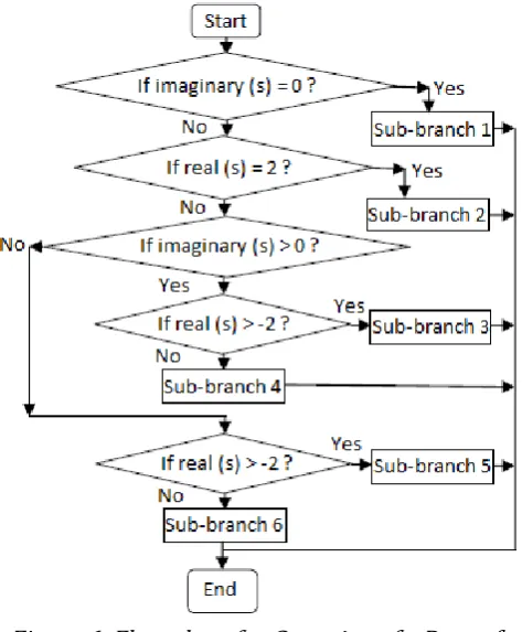
There are four branches starting from the four poles and ending at ∞. For the purpose of grouping into sub-branches, six sub-branches are identified. branch 1 is on the real axis. Sub-branch 2 is parallel to the imaginary axis at s=−2. Sub-branches 3 and 4 are above the real axis and are to the right and left of Sub-branch 2 respectively. Sub-branches 5 and 6 are below the real axis and are to the right and left of Sub-branch 2 respectively. Figure 6 shows the flow chart for grouping of root of this system into a sub-branch.

3.4 Comparison with Existing Technique 3.4 Comparison with Existing Technique 3.4 Comparison with Existing Technique 3.4 Comparison with Existing Technique

One of the existing techniques is the ‘rlocus’ code in Matlab [25]. The results obtained in this work are compared with the results obtained with the existing Matlab ‘rlocus’ code. Table 5 shows that the roots obtained by iteration in this work are exactly the same as those obtained using an existing Matlab ‘rlocus’ Code for three different open-loop transfer functions. The selected pair of iteration formulas developed in this work can be adapted to determine roots of equations for other applications besides root-locus.

(a)Root-Locus Dots-Plot

(b) Complete Root-Locus with details Figure 5: Root-Locus with details for

) 20 4 )( 4 ( ) ( )

( ₂

+ + + =

s s s s

K s

(9)

68

Table 3: Sample Root-Locus Plots Obtained

S/ N

Sample Plot S/

N

Sample Plot

1.

) 2 (

) 3 ( ) ( ) (

+ + =

s s

s K s H s

G 2.

) 2 2 )( 1 (

) 3 )( 2 ( ) ( )

( ₂

+ + +

+ + =

s s s s

s s K s H s G

3.

) 13 4 )( 4 )( 2 (

) 2 2 )( 3 )( 1 ( ) ( )

( 2

2

+ + + +

+ + + + =

s s s s s

s s s s K s H s

G 4.

) 5 )( 1 ( ) ( ) (

+ + =

s s s

K s

H s G

5.

) 5 )( 3 )( 2 (

) 4 )( 1 ( ) ( )

( ₂

+ + +

+ + =

s s s s

s s K s H s

G 6.

) 18 6 )( 6 ( ) ( ) (

2₊ ₊

+ =

s s s s

K s

H s G

(10)

69

Table 4: Details for

) 20 4 )( 4 ( ) ( )

( 2

+ + + =

s s s s

K s

H s G

S/N Description Results

1 Open-loop poles p1=0;p2 =−2 ;

4 2 ; 4

2 4

3 j p j

p =− − =− +

2 Open-loop zeros Nil

3

Point of intersection of asymptotes

2 − = s

4

Angles between the four

asymptotes and real axis

45o_{, 135}o_{, 225}o_{and 315}o

5 Breakaway points

2

− =

s (K =64);

45 . 2 2 j

s=− − (K=100) 2

− =

s (K=64); and

45 . 2 2 j

s=− + (K=100)

6

Value of K obtained for marginal stability

260 = K

7 Imaginary

crossover s=−j3.16and s=+j3.16 8 Additional roots

for K=260

16 . 3 4 j

s=− − and 16 . 3 4 j s=− +

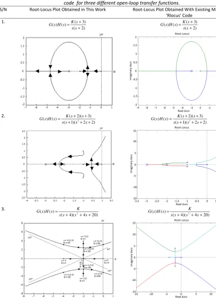
Table 6 compares the root-locus plots obtained in this work and those obtained using an existing Matlab ‘rlocus’ Code for three different open-loop transfer functions. The plots are the same in terms of shape and values of roots. The plots obtained in this work are magnified as the range of the plots along the real axis is controlled and limited to x≤real(s)≤+0.5. x is negative and is less than the real part of each of the open-loop poles and zeros. This is sufficient as the system is unstable in the range real(s)≥+0.5and the plot is predictable in the range−∞≤real(s)≤x. However, the user of the Matlab ‘rlocus’ code do not have

such convenient control over the range of the plot along real axis.

The input to the algorithm developed in this work can be either open-loop poles and zeros or transfer function expressed as the ratio of two polynomials. This is because it included an expansion process (section 2.1). This is an advantage over the existing Matlab ‘rlocus’ code which only accept transfer function expressed as the ratio of two polynomials. Furthermore, the developed algorithm adds details of asymptotes, breakaway points and imaginary axis crossover to the root-locus plot (section 2.4). This is another advantage over the existing Matlab ‘rlocus’ code.

Figure 6: Flow chart for Grouping of a Root of

) 20 4 )( 4 ( ) ( )

( 2

+ + + =

s s s s

K s

H s

G into a Sub-Branch.

Table 5: Comparison of roots obtained in this work and those obtained using existing Matlab ‘rlocus’ code for three different open-loop transfer functions.

) 2 (

) 3 ( ) ( ) (

+ + =

s s

s K s H s G

K = 1.2

) 2 2 )( 1 (

) 3 )( 2 ( ) ( )

( ₂

+ + +

+ + =

s s s s

s s K s H s G

K = 0.2

) 20 4 )( 4 ( ) ( )

( ₂

+ + + =

s s s s

K s

H s G

K = 3.55 Iteration

Results

Existing Matlab ‘rlocus’ Code

Iteration Results

Existing Matlab ‘rlocus’ Code

Iteration Results Existing Matlab ‘rlocus’ Code

1st_root _-1.6+j1.02 _-1.6+j1.02 _-1.061+j0.67 _-1.061+j0.67 _2.0+j3.978 _2.0+j3.978

2nd_root _-1.6-j1.02 _-1.6-j1.02 _-1.061-j0.67 _-1.061-j0.67 _2.0-j3.978 _2.0-j3.978

3rd_root _{-0.439+j0.755} _{-0.439+j0.755} _-3.955 _-3.955

(11)

70

Table 6: Comparison of root-locus plots obtained in this work and those obtained using existing Matlab ‘rlocus’ code for three different open-loop transfer functions.

S/N Root-Locus Plot Obtained in This Work Root-Locus Plot Obtained With Existing Matlab

‘Rlocus’ Code 1.

) 2 (

) 3 ( ) ( ) (

+ + =

s s

s K s H s G

) 2 (

) 3 ( ) ( ) (

+ + =

s s

s K s H s G

2.

) 2 2 )( 1 (

) 3 )( 2 ( ) ( )

( ₂

+ + +

+ + =

s s s s

s s K s H s G

) 2 2 )( 1 (

) 3 )( 2 ( ) ( )

( ₂

+ + +

+ + =

s s s s

s s K s H s G

3.

) 20 4 )( 4 ( ) ( ) (

2

+ + + =

s s s s

K s

H s G

) 20 4 )( 4 ( ) ( ) (

2

+ + + =

s s s s

K s

H s G

4. Conclusion 4. Conclusion 4. Conclusion 4. Conclusion

A computer aided root-locus numerical technique based on simple fast mathematical iteration has been developed. The technique has been tested successfully. The geometric properties of the root locus obtained with this technique are found to

(12)

71

5. 5. 5.

5. ReferencesReferencesReferencesReferences

[1] Chen, C. T. Analog and Digital Control System

Design, Saunders College, Orlando, Fla, USA, 1993.

[2] D’Azzo, J. J. and Houpis, C. H. Linear Control

System Analysis and Design: Conventional and Modern, McGraw-Hill, New York, NY, USA, 1995.

[3] Dorf, R. C. and Bishop, R. H. Modern Control Systems, Addison-Wesley, Reading, Mass, USA, 1998.

[4] Nagrath, I.J. and Gopal, M. Control Systems Engineering, Wiley Eastern Ltd, New Delhi, India, 1975.

[5] Ogata, K. Modern Control Engineering,

Prentice-Hall, Upper Saddle River, NJ, USA, 2001.

[6] Anih, L.U. and Amah, O. “The performance characteristics of a closed loop, one axis

electromechanical solar tracker”, Nigerian Journal

of Technology, Vol. 25, Number 2, 2006, pp. 66-76.

[7] Oti, S.E. and Okoro, O.I. “Stability analysis of static

slip-energy recovery drive via eigenvalue

method”, Nigerian Journal of Technology, Vol. 26, Number 2, 2007, pp. 13-29.

[8] Itaketo, U.T., Ogbogu, S.O.E. and Chukwudebe, G.A. “Apllication Of Lyapunov's Second Method In The Stability Analysis Of Oil/Gas Separation Process”, Nigerian Journal of Technology, Vol. 21, Number 1, 2002, pp. 60-71.

[9] Evans, W. R. “Control system synthesis by root

locus method”, Transactions of the American

Institute of Electrical Engineers, Vol. 69, Number 1, 1950, pp. 66–69.

[10] Evans, W. R. “Graphical analysis of control

systems,” Transactions of the American Institute

of Electrical Engineers, Vol. 67, Number 1, 1948, pp. 547–551.

[11] Krall, A. M. “The root locus method: a survey”,

SIAM Review, Vol. 12, Number 1, 1970, pp. 64–72.

[12] Pan, C.T. and Chao K.S. ‘’A Computer-Aided

Root-Locus Method’’, IEEE Transactions on Automatic

Control, Vol. AC-23, Number 5, October 1978, pp 856-860.

[13] Berman G. and Stanton, R. G. “The asymptotes of the root locus”, SIAM Review, Vol. 5, Number 3, 1963, pp. 209–218.

[14] Byrnes, C. I., Gilliam, D. S. and He, J. “Root-locus and boundary feedback design for a class of

distributed parameter systems”, SIAM Journal on

Control and Optimization, Vol. 32, Number 5, 1994, pp. 1364–1427, 1994.

[15] Eydgahi, A. M. and Ghavamzadeh, M.

“Complementary root locus revisited”, IEEE

Transactions on Education, Vol. 44, Number 2, 2001, pp. 137–143.

[16] Monteiro, L. H. A. and Da Cruz, J. J. “Simple answers to usual questions about unusual forms

of the Evans’ root locus plot”, Controley

Automacao, Vol. 19, Number 4, 2008, pp. 444–449.

[17] Bahar, E. and Fitzwater, M. “Numerical technique to trace the loci of the complex roots of

characteristic equations”, SIAM Journal on

Scientific and Statistical Computing, Vol. 2, Number 4, 1981, pp. 389–403.

[18] Krall, A. M. “A closed expression for the root locus

method”, SIAM Journal on Applied Mathematics,

Vol. 11, Number 3, 1963, pp. 700–704.

[19] Merrikh-Bayat, F. and Afshar, M. “Extending the root-locus method to fractional-order systems”,

Journal of Applied Mathematics, Vol. 2008, Article ID 528934, 2008, pp1-13.

[20] Merrikh-Bayat, F., Afshar, M. and Karimi-Ghartemani, M. “Extension of the root-locus method to a certain class of fractional-order

systems”, ISA Transactions, Vol. 48, Number 1,

2009, pp. 48–53.

[21] Spencer, D. L., Philipp, L. and Philipp, B. “Root loci

design using Dickson’s technique”, IEEE

Transactions on Education, Vol. 44, Number. 2, 2001, pp. 176–184.

[22] Teixeira, M. C. M., Assuncao, E. and Machado, E. R. M. D. “A method for plotting the complementary root locus using the root-locus _positive gain_ rules”, IEEE Transactions on Education, Vol. 47, Number 3, 2004, pp. 405–409.

[23] Teixeira, M. C. M., Assuncao, E., Cardim, R., Silva,

N.A.P. and Machado,E. R. M. D. “On

Complementary Root Locus of Biproper Transfer

Functions”, Journal of Applied Mathematics, Vol.

2009, Article ID 727908, 20091, pp 1-4.

[24] Anyaegunam, A. J. “Simple formulae for the evaluation of all the exact roots (real and

complex) of the general cubic”, Nigerian Journal of

Technology, Vol. 27, Number 1, 2008, pp. 48-53.

[25] MathWorks (Matlab), Documentation for

MathWorks products retrieved on January 1, 2009

from http://www.mathworks.com

/access/helpdesk/help/helpdesk.shtml

[26] Kelley, C. T. Iterative Methods for Linear and

Nonlinear Equations, SIAM, Philadelphia 1995.

[27] Onyia, O. T., Madueme, T. C. and Omeje, C. O. “An improved voltage regulation of a distribution network using facts - devices”, Nigerian Journal of Technology, Vol. 32, Number 2, 2013, pp. 304-317.