New Fifth-order Simpson-type Method for Solving Nonlinear Equations

New Fifth-order Simpson-type Method for Solving

Nonlinear Equations

R. Thukral

Padé Research Centre, 39 Deanswood Hill, Leeds, West Yorkshire, LS17 5JS, England

Abstract

The objective of this paper is to present further development of the Simpson-type methods for finding zeros of a nonlinear equation. The new Simpson-type method is shown to converge of the order five. Per iteration the new method requires the same amount of evaluations of the function and therefore the new method has an efficiency index better than the other similar Simpson-type methods. We examine the effectiveness of the new fifth-order Simpson-type method by approximating the simple root of a given nonlinear equation. Numerical comparisons are made to show the performance of the new iterative method and thus verifies the theoretical results.

Keywords

Simpson method, Newton method, Simple root, Nonlinear equation, Root-finding, Order of convergence

1. Introduction

In this paper, we present a new fifth-order iterative method to find a simple root of the nonlinear equation. It is well known that the techniques to solve nonlinear equations have many applications in science and engineering. We shall utilise two well-known techniques, namely the classical Newton method and the classical Simpson method, for their simplicity with convergence order of two and three respectively [1-13]. The new Simpson-type method requires the same amount of evaluations of the function as the classical Simpson method. Hence, we shall prove that the new Simpson-type iterative method has a better efficiency index than the other similar Simpson-type methods [1, 2, 4-7, 10, 12]. The prime motive for the development of the new fifth-order Simpson-type method was to increase the order of convergence of the recently introduced fourth-order Simpson-type methods.

2. The Method and Convergence

Analysis

Let f x

 

be a real function with a simple root



and let

 

x_n be a sequence of real numbers that converge towards



. The order of convergence p is given by * Corresponding author:

[email protected] (R. Thukral)

Published online at http://journal.sapub.org/ajcam

Copyright©2018The Author(s).PublishedbyScientific&AcademicPublishing This work is licensed under the Creative Commons Attribution International License (CC BY). http://creativecommons.org/licenses/by/4.0/



1



lim





0,



 



  

n p n

n

x x

(1)

where p and



is the asymptotic error constant. Also, let e_k x_k be the error in the kth iteration. Then the relation

 

1

1



,

   p  p

k k k

e e e (2) is the error equation. If the error equation exists, then p is the order of convergence of the iterative method [3, 8, 9, 13].

Furthermore, the efficiency of the method is measured by the concept of efficiency index, given by

 

, r ,

EI r p p (3) where r is the number of function evaluations of the method and p is the order of the convergence of the method [8]. In order to approximate the order of convergence of the method we use the following formula. Suppose that x_n1,x_n and

1



n

x are three successive iterations closer to the root



of (1). Then the computational order of convergence may be approximated by

1

1 2

ln COC

ln











 

 



n n

n n

, (4)

where



_i  f x

 

_i f

 

x_i , [11].

2.1. The Classical Simpson Third-order Method

Since this method is well established, we shall state the essential expressions used in order to calculate the root of the given nonlinear equation. Hence the Simpson third-order method is given as

 

 

 

 

1 6 , 4

   _{  } n _{ }

n n

n n n

f x

x x

f x f z f y (5)

where

 

 

,   n n n f x u

f x (6)

,  

n n n

y x u (7) 1

2 ,

 

n n n

z x u (8)

0

x is the initial approximation and provided that the denominator of (5) is not equal to zero.

2.2. The Simpson-type Fourth-order Methods

In this section we state the recently introduced fourth-order Simpson-type method to find simple root of a nonlinear equation. The improvement of the classical Simpson method was made by introducing a new factors in (5). Hence, the improved fourth-order Simpson-type methods is given by

 

 

 

 

 

1 6 4    _{    } i n n n

n n n

f x

x x

f x f z f y

 

2

2 3

2 





 _{ } _   i n n u

f x (9)

where m,

 

 





1 2

,



  n   n

n

f y f z

u (10)

 

 





2 2

,



  n   n

n

f x f z

u (11)

 

 

 

3

5 4

, 3



  n   n   n

n

f x f z f y

u (12)

 

 

 





4 4 3 , 1 2



        

n n n

n n n

f z f y f x

m w mv mu (13)

 

 

,   n n n f x v

f y (14)

 

 

.   n n n f x w

f z (15)

Further details of the above methods are given in [12].

2.3. New Simpson-type Fifth-order Method

Here we present a new scheme to find simple root of a nonlinear equation. In order to increase the order of convergence of the classical Simpson method and the fourth-order Simpson-type method, we shall introduce a new different type of factor in (5). Hence, the scheme of the new fifth-order Simpson method is given by

 

 

 

 

1

6

4

   _{  } n _{ }

n n

n n n

f x

x x

f x f z f y

 

 

2 3

2 3 1 4

2 



 2 



 ,

 _{ } _  _{ } _

 n  n  n  n

u u

f x f x (16)

alternatively the new formula maybe expressed as

 

 

 

 

1

6

4

   _{  } n _{ }

n n

n n n

f x

x x

f x f z f y

 

 

2

2 3

2 



 1 2



 ,

 _ _   _ _ 

 _  _

 n  n  n  n 

u u

f x f x (17)

where u_n is given by (6) and

 

 

.



  n   n

n

f x f y

u (18)

Theorem 1

Let



D be a simple zero of a sufficiently differentiable function f D:     for an open interval D. If the initial guess x₀ is sufficiently close to



, then the order of convergence of the new Simpson-type method defined by (16) is five.

Proof

Let



be a simple root of f x

 

, i.e. f

 



0 and

 



0

 

f , and the error is expressed as



 

e x . (19) Using Taylor expansion, we have

 

 

1

 

2

( _n)



 



_n2 



_n

f x f f e f e (20)

Taking f

 



0 and simplifying, expression (20) becomes

 

 

2 3

2 3



 



 _    _

n n n n

f x f e c e c e . (21) where  

_{ }

   

!





  k k f c

Furthermore, we have

 

 

2

2 3

1 2 3 .



 

 _n   _  _n _n _

f x f c e c e (23)

Dividing (21) by (23), we get

 

 

  2 22



22 3



3

 n

n n n

n

f x

e c e c c e

f x (24)

and hence, we have

 

 

2 2 2



22 3



3

     

 n

n n n n

n

f x

y e c e c c e

f x (25)

The expansion of f

 

y_n about



is given as

 

 

2



2



3

2 2 2 3 .



 

 _n   _{ n}  _n _

f y f c e c c e (26)

Since from (8) we have

 

 

2

1 2

2

2 2

  

  _{ } _  

 

n n n

n n

n

f x e c e z x

f x (27)

Taylor expansion of f

 

z_n about



is

 

 

2



2



3

2 2 2 3 .



 

 _n   _{ n}   _n _

f z f c e c c e (28)

The denominator of (5) is given as

 

4

 

 

 _n   _n   _n

f x f z f y



2



2

2 2 3

6 6 6

  c e_n c c e_n (29)

Dividing the numerator by denominator of (5), we get





2 3 3 4

2 3 2 2 3

   

n n n

e c e c c c e (30) It is well established that the error equation of (5) is





2 3 3 4

1 2 3 2 2 3

    

n n n

e c e c c c e (31) The improvement factors introduce in (16) are

 

 

2 3

2 3 ,



  n   n   

n n

f x f y

c c e

u (32)

 





2

2 3 2 3 3 4

2 2 3 2

2 _



_   3 7  ,



 n  n n n

u c e c c c e

f x (33)

 





3

1 4 3 4 2 4 5

2 2 3 2

2 _



_ 4 2 9 20 



 n  n n n

u c e c c c e

f x (34)

Substituting appropriate expressions in (16), we obtain





2 4 2 5

1 2 52 2 3 

   

n n

e c c e (35) The error equation (35) establishes the fifth-order convergence of the new iterative method defined by (16).

3. Numerical Test Examples

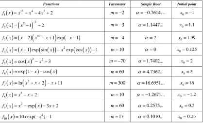
Table 1. Test functions and their simple roots

Functions Parameter Simple Root Initial point

 

15 4 2

1   4 2

f x x x x m 2   0.7614 x0 1

 



₃



1

2 1 2



  

f x x m 3  1.1447... x01.1

  





10







3  2  1 exp  1

f x x x x x m 4 2 x01.99

  





 



2



 



4  1 exp sin  exp cos 1

f x x x x x m10 0 x00.125

 

 

2 2

5 cos  3

f x x x m 70 1.7402... x02

 





 

6 exp 1 cos

f x x x m60  4.7362... x05

 



2



7 ln  2  11

f x x x x m300  16.6951... x016

 

5

8   2

f x x x m10   1.2671... x0 1.2

 

2

 

9  exp 3 2

f x x x x m60 0.2575... x0 0.5

 

2

10 10 exp( ) 1

Table 2. Errors occurring in the estimates of the simple root by the methods described

i

f (5) (9):i=1 (9):i=2 (9):i=3 (9):i=4 (16)

1

f 0.785e-31 0.807e-56 0.791e-75 0.537e-97 0.230e-113 0.503e-138

2

f 0.139e-41 0.620e-89 0.574e-106 0.445e-102 0.588e-148 0.146e-202

3

f 0.720e-113 0.473e-296 0.115e-308 0.292e-306 0.208e-312 0.679e-685

4

f 0.318e-90 0.959e-216 0.932e-253 0.149e-243 0.194e-319 0.315e-509

5

f 0.130e-160 0.280e-344 0.386e-331 0.367e-347 0.139e-435 0.532e-748

6

f 0.865e-147 0.181e-311 0.129e-289 0.537e-304 0.221e-336 0.291e-716

7

f 0.172e-205 0.441e-567 0.192e-545 0.107e-556 0.252e-571 0.650e-1318

8

f 0.689e-74 0.880e-166 0.124e-181 0.148e-178 0.804e-253 0.174e-364

9

f 0.751e-138 0.319e-325 0.248e-351 0.517e-374 0.192e-406 0.342e-908

10

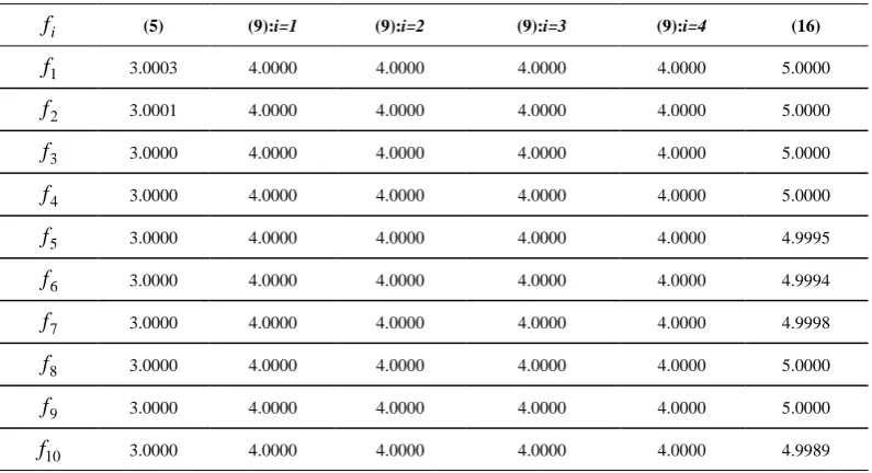
f 0.130e-93 0.176e-274 0.745e-200 0.274e-210 0.871e-284 0.259e-521 Table 3. Performance of computational order of convergence

i

f (5) (9):i=1 (9):i=2 (9):i=3 (9):i=4 (16)

1

f 3.0003 4.0000 4.0000 4.0000 4.0000 5.0000

2

f 3.0001 4.0000 4.0000 4.0000 4.0000 5.0000

3

f 3.0000 4.0000 4.0000 4.0000 4.0000 5.0000

4

f 3.0000 4.0000 4.0000 4.0000 4.0000 5.0000

5

f 3.0000 4.0000 4.0000 4.0000 4.0000 4.9995

6

f 3.0000 4.0000 4.0000 4.0000 4.0000 4.9994

7

f 3.0000 4.0000 4.0000 4.0000 4.0000 4.9998

8

f 3.0000 4.0000 4.0000 4.0000 4.0000 5.0000

9

f 3.0000 4.0000 4.0000 4.0000 4.0000 5.0000

10

f 3.0000 4.0000 4.0000 4.0000 4.0000 4.9989

The new fifth-order Simpson-type method given by (16) is employed to solve nonlinear equations with simple root. To demonstrate the performance of the new iterative method, ten particular nonlinear equations are used. The estimates are given of the approximate solutions produced by the methods considered and list the errors obtained by each of the methods. To determine the efficiency index of the new method, formula (3) will be used. Hence, the efficiency index of the new iterative method given by (16) is

4

51.4953, whereas the efficiency index of the fourth-order Simpson-type method given by (9) is

4

4 1.4142 and the efficiency index of the classical

Simpson third-order method is given by (5) is 431.3161. Ten particular test functions are displayed in Table 1. The difference between the simple root and the approximation

n

x for test functions with initial guessx₀are displayed in Table 2. In fact, x_n is calculated by using the same total number of function evaluations for all methods. Furthermore, we display the computational order of convergence approximations in Table 3. From the tables we observe that the computational order of convergence perfectly coincides with the theoretical result.

4. Conclusions

Simpson third-order iterative method and recently introduced the Simpson-type fourth-order iterative methods. It is shown that the efficiency index of the new fifth-order method is much better than the fourth-order Simpson-type method and the classical Simpson third-order method. Numerical comparisons are made to demonstrate the performance of the derived method. We have examined the effectiveness of the new fifth-order iterative method by showing the accuracy of the simple root of a nonlinear equation.

REFERENCES

[1] N. Ahmad, V. P. Singh, A New Iterative Method for Solving Nonlinear Equations Using Simpson Method, Inter. J. Math. Appl. 5 (4) (2017) 189–193.

[2] Eskandari, H. Simpson’s Method for Solution of Nonlinear Equation. Appl. Math. 8 (2017) 929-933.

[3] W. Gautschi, Numerical Analysis: an Introduction, Birkhauser, 1997.

[4] V. I. Hasanov, I. G. Ivanov, G. Nedjibov, A New modification of Newton’s method, Appl. Math. Eng (2015) 278-286.

[5] J. Jayakumar, Generalized Simpson-Newton's Method for Solving Nonlinear Equations with Cubic Convergence, J. Math. 7 (5) (2013) 58-61.

[6] G. Nedjibov, V. I. Hasanov, M. G. Petkov, On some families of multi-point iterative methods for solving nonlinear equations, Numer. Algo. 42 (2) (2006) 127-136.

[7] A. M. Ostrowski, Solutions of equations and system of equations, Academic Press, New York, 1960.

[8] S. Nazneem, A new approach of Newton’s method using Simpson’s rule, Asian J. Appl. Sci. Tech. 2 (1) (2018) 135-138.

[9] M. S. Petkovic, B. Neta, L. D. Petkovic, J. Dzunic, Multipoint methods for solving nonlinear equations, Elsevier 2012. [10] U. K. Qureshi, A new accelerated third-order two-step

iterative method for solving nonlinear equations, Math. Theory Model. 8 (5) (2018) 64-68.

[11] R. Thukral, New modifications of Newton-type methods with eighth-order convergence for solving nonlinear equations, J. Adv. Math. Vol 10 (3) (2015) 3362-3373.

[12] R. Thukral, Further acceleration of the Simpson method for solving nonlinear equations, J. Adv. Math. Vol 14 (2) (2018) 7631-7639.