Atmospheric inversion of surface carbon flux with consideration of the spatial distribution of US crop production and consumption

www.biogeosciences.net/12/323/2015/ doi:10.5194/bg-12-323-2015

© Author(s) 2015. CC Attribution 3.0 License.

Atmospheric inversion of surface carbon flux with consideration of

the spatial distribution of US crop production and consumption

J. M. Chen1,2, J. W. Fung2, G. Mo2, F. Deng3, and T. O. West4

1_{International Institute of Earth System Science, Nanjing University, Nanjing, Jiangsu, China}

2_{Department of Geography and Program in Planning, University of Toronto, Toronto, Ontario, M5S 3G3, Canada} 3_{Department of Physics, University of Toronto, Toronto, Ontario, M5S 3G3, Canada}

4_{Joint Global Change Research Institute, Pacific Northwest National Laboratory, College Park, Maryland, USA} Correspondence to: J. M. Chen, ([email protected])

Received: 26 November 2013 – Published in Biogeosciences Discuss.: 29 April 2014 Revised: 15 September 2014 – Accepted: 3 December 2014 – Published: 19 January 2015

Abstract. In order to improve quantification of the spatial distribution of carbon sinks and sources in the contermi-nous US, we conduct a nested global atmospheric inver-sion with detailed spatial information on crop production and consumption. County-level cropland net primary productiv-ity, harvested biomass, soil carbon change, and human and livestock consumption data over the conterminous US are used for this purpose. Time-dependent Bayesian synthesis inversions are conducted based on CO2observations at 210

stations to infer CO2 fluxes globally at monthly time steps

with a nested focus on 30 regions in North America. Prior land surface carbon fluxes are first generated using a bio-spheric model, and the inversions are constrained using prior fluxes with and without adjustments for crop production and consumption over the 2002–2007 period. After these adjust-ments, the inverted regional carbon sink in the US Midwest increases from 0.25±0.03 to 0.42±0.13 Pg C yr−1, whereas the large sink in the US southeast forest region is weak-ened from 0.41±0.12 to 0.29±0.12 Pg C yr−1. These ad-justments also reduce the inverted sink in the west region from 0.066±0.04 to 0.040±0.02 Pg C yr−1because of high crop consumption and respiration by humans and livestock. The general pattern of sink increases in crop production areas and sink decreases (or source increases) in crop consumption areas highlights the importance of considering the lateral car-bon transfer in crop products in atmospheric inverse model-ing, which provides a reliable atmospheric perspective of the overall carbon balance at the continental scale but is unreli-able for separating fluxes from different ecosystems.

1 Introduction

Human activities have greatly modified the global carbon cy-cle through fossil fuel consumption, cement production, and land use (Canadell et al., 2007; Le Quéré et al., 2013). The airborne fraction of these carbon sources has been highly variable from year to year, mostly due to large variations in the terrestrial carbon sink (Le Quéré et al., 2009, 2013). Due to the complexity and heterogeneity of land cover, it has been a challenge to estimate the spatial distribution and magnitude of terrestrial carbon sources and sinks. It has been more re-liable thus far to derive the terrestrial sink as a residual of the global carbon budget than to estimate it using land-based data (Le Quéré et al., 2013). Our ability to project the car-bon cycle and estimate its influence on climate will remain limited if we cannot resolve the current carbon source and sink distribution patterns and provide plausible mechanistic explanations for the patterns. In this regard, regional stud-ies that focus on the spatial distribution of carbon dynamics would be a useful direction for improving our understanding of the global carbon cycle.

al., 2002, 2003, 2004; Rödenbeck et al., 2003; Baker et al., 2006; Peters et al., 2007; Deng et al., 2013; Peylin et al., 2013), while 19 biospheric models (referred to as “bottom-up”) produced an average sink of 0.6 Pg C yr−1, with a range from−0.7 to 2.2 Pg C yr−1, for North America over the pe-riod from 2000 to 2005 (Huntzinger et al., 2012). Using a biospheric model, Turner et al. (2013) estimated that the net ecosystem productivity (NEP) over North America in 2004 was 1.73±0.37 Pg C yr−1, and this NEP value is reduced by 0.616 Pg C yr−1 for the carbon loss due to harvested prod-uct emission, river/stream evasion, and fire emission in order to estimate the total land sink. These top-down and bottom-up estimates at the continental scale broadly agree, giving us confidence that North America is a large and important con-tributor to the global terrestrial carbon sink.

With respect to the spatial distribution of the North Amer-ican carbon sink, results become more uncertain at higher spatial resolutions. Disaggregation of the sink between North American boreal and temperate regions is plagued with un-certainties. For the boreal region, an inversion study (Fan, 1998) produced a sink of 0.2±0.4 Pg C yr−1in 1988–1992, while a TransCom 3 experiment (Gurney et al., 2003) showed a source of 0.26±0.39 Pg C yr−1 in 1992–1996. When the TransCom 3 experiment was repeated with updated data, it became a sink of 0.003±0.28 Pg C yr−1 in 1992–1996 (Yuen et al., 2005). Using forest inventory data, Canadian forests were found to be a carbon source of 0.069 Pg C yr−1 in 1985–1989 (Kurz and Apps, 1999), while (Pan et al., 2011a) estimated that forests in Canada and Alaska were a carbon sink of 0.26±0.06 Pg C yr−1 in 1990–2008. A bio-spheric model calculated a weak sink of 0.05 Pg C yr−1for Canadian forests during the 1980s to 1990s (Chen et al., 2003). For the conterminous US, with approximately 32 % of the total North America area, estimates of the sink from a set of bottom-up and top-down methods fall in a range from 0.30 to 0.58 Pg C yr−1 in 1980–1989 (Pacala et al., 2001), while TransCom 3 experiments inferred the sink in 1992– 1996 to be 0.89±0.22 and 0.82±0.40 Pg C yr−1for inver-sions at monthly and annual time steps, respectively (Gur-ney et al., 2003, 2004; Baker et al., 2006). These differences suggest that uncertainty due to the temporal resolution of in-verse modeling is considerable. Peters et al. (2007) devel-oped a carbon assimilation system implemented at weekly time steps, referred to as CarbonTracker (CT), and showed that the sink in 2000–2005 in temperate North America was 0.50±0.60 Pg C yr−1. With a simple atmospheric bud-geting approach applied to CO2 measurements in the

in-flows and outin-flows through the troposphere over the con-terminous US, Crevoisier et al. (2010) deduced a sink of 0.5±0.4 Pg C yr−1 in 2004–2006. Seven other inversion studies, on average, indicate that temperate North America was a sink of 0.685±0.574 Pg C yr−1 in 2000–2006 (see summary in Hayes et al., 2012). Although these estimates have large uncertainties, they generally indicate that the

ma-jor sink in North America is located in the temperate region while the boreal region is either a small sink or source.

The locations of carbon sinks and sources within tem-perate North America are highly uncertain. The 19 bio-spheric models employed by Huntzinger et al. (2012) gen-erated very different sink and source spatial patterns over the conterminous US, although the average sink mostly ap-pears in forested areas in southeast, northeast and northwest regions. Another bottom-up estimate using long-term mod-eling and recent remote sensing inputs suggested that forests in the southeast region are large sinks because of their pre-dominant mid-age structure (Zhang et al., 2012). Based on forest inventory data, Williams et al. (2012) deduced that forests along the east and west coasts of the US were large sinks in 2005–2006, with most areas in the southeast region (i.e., Arkansas, Louisiana, Mississippi, and Alabama) having sinks in the range of 110–140 g C m−2yr−1. However, Car-bonTracker (Peters et al., 2007) repeatedly produces large sinks in cropland and adjacent grassland areas, while the southeast region varied between being a small source and a small sink. Inversion studies that divide North America into 30 regions (11 in the conterminous USA; Deng et al., 2007; Deng and Chen, 2011) indicate broad patterns of the sink distribution in both the southeast forest and Midwestern crop regions. In these two studies, the seasonal variations of the carbon flux from various terrestrial ecosystems modeled by a biospheric model and neutralized at the annual time step were used as the prior flux to constrain the inversion. Under the neutralized flux constraint, the inverted sink may be more or less regarded as the atmospheric signal, although the inver-sion results are inevitably influenced by errors in transport modeling and other prior fluxes such as fossil fuel, biomass burning, and ocean–atmospheric exchange. Inversion stud-ies by Peters et al. (2007), Deng and Chen (2011), Lauvaux et al. (2012), and Schuh et al. (2013) indicate that the mid-west croplands persistently behave as a large regional sink, but this sink generally does not accumulate locally in soil and vegetation due to lateral transfer of agricultural products and therefore could not be estimated from the local carbon stock changes. From the atmospheric perspective, crop pro-duction during the growing season results in large uptake of CO2 from the atmosphere, while crop consumption

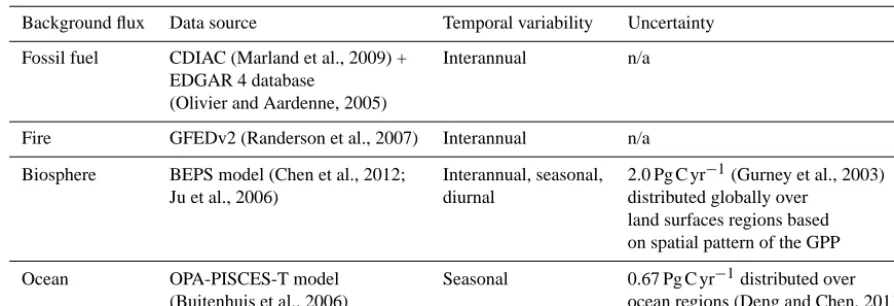
Table 1. Summary of background prior fluxes and their uncertainties.

Background flux Data source Temporal variability Uncertainty

Fossil fuel CDIAC (Marland et al., 2009) + Interannual n/a

EDGAR 4 database

(Olivier and Aardenne, 2005)

Fire GFEDv2 (Randerson et al., 2007) Interannual n/a

Biosphere BEPS model (Chen et al., 2012; Interannual, seasonal, 2.0 Pg C yr−1(Gurney et al., 2003)

Ju et al., 2006) diurnal distributed globally over

land surfaces regions based on spatial pattern of the GPP

Ocean OPA-PISCES-T model Seasonal 0.67 Pg C yr−1distributed over

(Buitenhuis et al., 2006) ocean regions (Deng and Chen, 2011)

need to be considered in both bottom-up and top-down mod-eling in order for them to converge on similar spatial patterns of the carbon sink and source distribution.

The necessity of including lateral transfer of carbon in the prior flux for constraining inverse modeling can be ques-tioned because it could be argued that atmospheric CO2

mea-surements have already integrated the outcome of all carbon cycle processes including the lateral movement of carbon both at the surface and in the atmosphere. Theoretically, this argument is well grounded if we have sufficient atmospheric CO2measurements, and it could possibly hold true for North

America, which is one of the most densely observed regions in the world with respect to atmospheric CO2. However, the

extent to which the carbon source and sink distribution over North America is determined by atmospheric CO2

measure-ments has not been systematically assessed. The Bayesian synthesis inversion framework, in which a prior flux is used to constrain the inversion (Enting, 2002), provides an ideal tool for this assessment. The extent to which the inverted flux distribution is influenced by the inclusion of lateral carbon transfer in the prior flux could be an indicator of the strength of existing atmospheric CO2measurements on the carbon

cy-cle relative to the prior flux.

In this study, we attempt first to include crop production and consumption information in the prior flux for constrain-ing our existconstrain-ing inverse modelconstrain-ing system (Deng and Chen, 2011) and then to assess the necessity of this inclusion for de-termining the carbon source and sink distribution over North America. The consumption of crop products by livestock and humans is about twice the consumption of forest products (West et al., 2011; Hayes et al., 2012). Unlike forest prod-ucts with a large range of residence times, crop prodprod-ucts can be assumed to be consumed within a year of harvest (West et al., 2011). The spatial distributions of crop production and consumption at the county level (West et al., 2011) provide a sufficient resolution for use in atmospheric inverse modeling. The specific objectives of our study are: (1) to investigate the changes in the inverted carbon source and sink distribution

after considering the spatial patterns of crop production and consumption, (2) to explore whether these changes improve our understanding of the carbon source and sink distribution within the conterminous US, (3) to evaluate the impact of the crop data on the inverted carbon balance for the contermi-nous US and other regions of the globe, and (4) to assess the relative importance of atmospheric CO2 data and the prior

flux in determining the spatial pattern of the carbon sink in the conterminous US.

2 Atmospheric CO2inversion methodology

The Bayesian synthesis inversion method (Enting and Trudinger, 1995) is used in this study. This method includes forward modeling of atmospheric CO2 concentration using

a transport model with prior fluxes and inverse modeling of the surface CO2flux based on the difference between

mod-eled and observed CO2concentrations.

2.1 Forward modeling

2.1.1 Prior fluxes and their uncertainties

The a priori fluxes needed in the Bayesian synthesis inversion include sources from fossil fuel emissions, fire emissions, net carbon exchange between atmosphere and land, and net car-bon exchange between atmosphere and ocean. These fluxes for the time period from 2000 and 2007 used in this study are the same as those used in Deng and Chen (2011) (Table 1). The fossil fuel emission field used in this study is constructed based on the fossil fuel CO2emission inventory from 1871 to

(a)

(b)

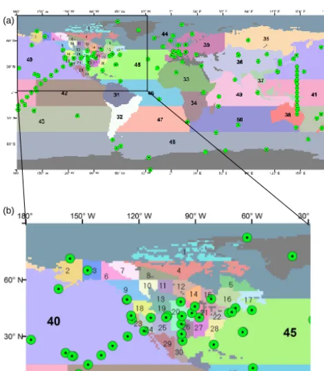
Figure 1. (a) A nested inversion system with 30 regions for North

America and 20 regions for the remainder of the globe. The 210 measurement sites are indicated as circles. (b) An enlarged portion for North America.

The Boreal Ecosystem Productivity Simulator (BEPS) is employed to produce seasonally varying net ecosystem ex-change (NEE) fluxes in hourly time steps globally (Chen et al., 1999, 2012; Ju et al., 2006). Developed based on FOR-EST Biogeochemical Cycles (FORFOR-EST-BGC) (Running and Coughlan, 1988), BEPS was originally intended for mod-eling the Canadian forest carbon cycle (Chen et al., 2007; Ju et al., 2006; Liu et al., 1999, 2002), but it has been ex-tended to temperate and tropical ecosystems (Higuchi et al., 2005; Matsushita and Tamura, 2002; Sun et al., 2004; Chen et al., 2012). It uses remotely sensed leaf area index (LAI) (Deng et al., 2006), land cover type from Global Land Cover (GLC2000), meteorology from NCEP-reanalysis (Kalnay et al., 1996), and soil textural data (Webb et al., 1991). A unique feature of BEPS is the separation of sunlit and shaded com-ponents in the canopy using not only LAI but also a foliage clumping index (Chen et al., 2005; He et al., 2012) when cal-culating photosynthesis (Liu et al., 2002; Chen et al., 2012). Given that soil carbon pools are often not well modeled by terrestrial biosphere models, large uncertainties exist in the modeled annual carbon fluxes. However these models are still useful in estimating seasonal and diurnal patterns in re-sponse to changes in environmental conditions. Therefore, in most atmospheric inversion studies the prior annual mean NEE from land surfaces at each grid is set to zero (Gurney et al., 2004; Rödenbeck et al., 2003). The use of seasonally

and diurnally varying biospheric fluxes is essential for the forward modeling to include the covariance of atmospheric transport and the surface flux (Denning et al., 1995; Gurney et al., 2004; Randerson et al., 1997; Deng and Chen, 2011).

In this study, two sets of control terrestrial biosphere fluxes from BEPS are prepared: (1) annually balanced but season-ally and diurnseason-ally varying NEE fluxes, and (2) annuseason-ally, sea-sonally, and diurnally varying NEE fluxes. The annually bal-anced NEE fluxes are prepared by forcing the annual mean NEE to be zero, resulting in no interannual variability, while the seasonal and diurnal variability is retained. In fulfilling the objectives of this research, cropland carbon adjustments are made to these prior NEE fluxes (see Sect. 3).

The main processes responsible for ocean CO2 uptake is

the partial pressure difference between the sea surface and the overlying air which in part depends on the seasonal growth of phytoplankton in the oceans. The daily air–sea CO2 fluxes across the sea surface in this research are

sim-ulated by the OPA-PISCES-T model, which is a global cir-culation model (OPA) (Madec et al., 1998) coupled with an ocean biochemistry model (PISCES-T) (Aumont, 2003; Buitenhuis et al., 2006). This coupled model is forced by daily wind stress, heat, and water fluxes from NCEP re-analysis (Kalnay et al., 1996). The ocean–atmosphere flux – along with the land–atmosphere flux, fossil emissions, and fire emissions – from 2000 to 2007 were fitted to a 1◦×1◦ spatial scale at hourly time steps and aggregated to 3◦×2◦ for North America and 6◦×4◦ for the rest of the globe as inputs for forward modeling.

2.1.2 Atmospheric transport

The atmospheric transport model chosen for this research is the transport-only version of the global chemistry transport model (Krol et al., 2005) version 5 (TM5), which is an offline model driven by meteorological data from the European Cen-tre for Medium-Range Weather Forecast (ECMWF) model. In this study, we define a global grid of 6◦×4◦with nested grids focusing on North America at 3◦×2◦based on Peters et al. (2005). The model consists of 25 vertical layers: 5 lay-ers in the boundary layer, 10 in the free troposphere, and 10 in the stratosphere. In this study, the prior hourly fluxes are input into TM5 to generate forward simulations of hourly concentrations at 210 CO2observation sites across the globe

for emissions from fossil fuel consumption (cff), fire (cfire),

terrestrial biosphere (cbio), and oceans (coce).

2.1.3 CO2observations

The atmospheric CO2concentrations used in this study are

the monthly CO2observation data from 2000 to 2007

com-piled in the GLOBALVIEW-CO22008 database. These

with different data types, including surface flask, tower, air-craft, and ship measurements. In this study, selected months that used measurement-based data from 210 stations are taken to compile the CO2concentration matrix, and they

con-sist of 12 181 station measurements during the 8-year period from 2000 to 2007 (Fig. 1).

In order to find the concentration corresponding to the bi-ases in the surface carbon flux to be adjusted through in-verse modeling, simulated concentrations corresponding to the prior fluxes need to be subtracted from CO2

measure-ments. For continental tower sites, the GLOBALVIEW-CO2

data set contains weekly averages of measurements in only afternoon hours to capture the well-mixed condition within the planetary boundary layer, and therefore the monthly sim-ulated concentrations at these sites are also taken as av-erage values in the same afternoon hours. For non-tower sites, GLOBALVIEW-CO2provides a summary of the

sam-ple collection times for discrete observations. The simulated concentrations are also sampled at the same times to ob-tain the monthly mean values, so as to be consistent with the GLOBALVIEW-CO2 data set. These monthly averaged

simulated concentrations are then subtracted from the cor-responding 12 181 monthly CO2 measurements (cobs) from

GLOBALVIEW-CO2to produce the residual concentration

(C), expressed as follows:

c=cobs−cff−cfire−cbio−coce. (1)

This residual concentration is used as input to the inversion system to optimize the surface carbon flux.

2.2 Inverse modeling

2.2.1 Inversion regions and concentration locations The atmospheric CO2concentrations are used for inversion

of 50 global regions, including 30 regions in North Amer-ica (Fig. 1), following Deng et al. (2007) and Deng and Chen (2011). The 30 regions in North America are delineated based on a 1 km resolution land cover map from AVHRR (Advanced Very High Resolution Radiometer) data (DeFries and Townshend, 1994) and provincial and state boundaries. This nested inversion system allows for a reduction of errors due to spatial aggregation over the focused region of North America and in the meantime does incur excessive computa-tion. Although the spatial resolution over North America is still relatively low, the number of regions is adequate to cap-ture the atmospheric signal and to show the broad source and sink patterns.

2.2.2 Time-dependent Bayesian synthesis approach In the time-dependent Bayesian synthesis approach (Enting, 2002) used in our inverse modeling, a linear combination of source and sink terms is formulated to match with CO2

con-centration observations:

c=Gf+Ac0+ε, (2)

wherec_m×1is a vector ofmatmospheric CO2observations

at given space and times; εm×1 is a random error vector

with a zero mean and a covariance matrixcov(ε)=Rm×m;

Gm×(n−1) is a given matrix representing a transport

(obser-vation) operator, where n−1 is the number of fluxes to be determined; Am×1is a unity vector (filled with 1) that relates

to the assumed initially well-mixed atmospheric CO2

con-centrations (c0); andf(n−1)×1is an unknown vector of

car-bon fluxes of all studied regions. In this research,m=12 181 (the number of measurements as mentioned in Sect. 2.1.3) and (n−1)=4800 (50 regions×8 years×12 months).

After combining matrixes G and A into Mm×n=(G,A)

and vectorsf andc0assn×1=(fT,c0)T, Eq. (2) is

rewrit-ten as

c=Ms+ε. (3)

while Eq. (3) can be solved forsby the conventional least-squared technique, the problem is poorly constrained. The Bayes approach (Tarantola, 2005) is generally used for ill-constrained problems through introducing a priori informa-tion in the inversion process. The best a priori informainforma-tion for this purpose is a prior estimate of the surface flux. The a posteriori flux is obtained by minimizing the following cost functionJ:

J=1

2(Ms−c)

T_R−1_(Ms−c)+1

2(s−sp)

T_Q−1_(s−s

p), (4)

wherespn×1 is the a priori estimate of s (set to zero after

subtracting its contribution to concentration from the atmo-spheric CO2observation); the covariance matrix Qn×n

repre-sents the uncertainty in the a priori estimate; andRm×mis the

model–data mismatch error covariance. Through minimizing this cost function in Eq. (4), the posterior best estimate ofs (Enting, 2002) is defined as

ˆ

s=(MTR−1M+Q−1)−1(MTR−1c+Q−1sp), (5)

with the posterior uncertainty expressed as follows: ˆ

Q=(Q−1+MTR−1M)−1. (6) 2.2.3 Transport (observation) operator, model–data

mismatch, and prior uncertainties

concentration at each observation site. The model–data mis-match, R, reflects the difference between the modeled and the observed CO2concentrations, which include both errors

from transport modeling and measurement (such as instru-ment errors). The observation sites were divided into five categories, each with its own constant portion (σconst) and

variable portion (GVsd) that is computed monthly from the standard deviation data given in GLOBALVIEW-CO22008

variation (var) files. The constant portion is defined under the following categories: Antarctic sites (0.15), oceanic sites (0.30), land and tower sites (1.25), mountain sites (0.90), and aircraft samples (0.75). The variable portion is the sta-tistical summary of average atmospheric variability for each measurement record. Therefore, the covariance matrix, R, is given as a diagonal matrix that contains the error for each monthi:

Rii=σconst2 +GVsd2. (7)

Additionally, a weighting factor, W, is inserted to the cost function in Eq. (4) to account for the vertical correlation be-tween measurements at different levels of the same tower and aircraft sites (i.e., smaller weights are given to each of the measurements at the same site) (Deng and Chen, 2011).

J =1

2((Ms−c)W )

T_R−1_{((Ms−c)W )}

+1 2(s−sp)

T_Q−1_(s−s

p) (8)

The weight,W, is a diagonal matrix with the diagonal terms given by

wii=1/(1+0.6(n−1)), (9)

wherenis the number of observations at different levels at the same site.

While the a priori fluxes are set to zero after subtracting their contributions toward the measured CO2concentrations,

the a priori uncertainties, Q, are important in forcing the spa-tial distribution of the inverted fluxes (Table 1). The uncer-tainties for fossil fuel of ±6 % (Marland et al., 2009) and for fire fluxes of±20 % (van der Werf et al., 2010) are not included in Q, and hence, it is important to note that the in-verted fluxes are subject to these additional uncertainties.

Theχ2test (Gurney et al., 2003) is employed to test the consistency of the fit to CO2data and the prior flux estimate

simultaneously:

χ2=Jmin Nobs

=

m P

m=1

(Ms−c)2

R2 +

n P

n=1

(s−sp)2

Q2

Nobs

, (10)

whereNobsis the number of degrees of freedom andJminis

the cost function from Eq. (4). The consistency of the fit is highest when the value ofχ2equals unity.

3 US cropland carbon integration methodology During the growing season, cropland in the US Midwest rep-resents a strong regional carbon sink. However, a large por-tion of crop biomass is removed during harvest and trans-ported to other regions for processing and consumption. When the crop products are consumed by humans and live-stock, CO2 is released back into the atmosphere at

geo-graphic locations that differ from the origin of production. In this study, these lateral redistributions of carbon are con-sidered in the prior fluxes used in atmospheric CO2inversion

studies in order to investigate their influence on the inverted carbon source and sink distribution.

3.1 US cropland carbon budget based on inventory data

The regional patterns of CO2uptake and release in US

crop-lands based on agricultural statistics (West et al., 2011) are used to adjust the prior biosphere flux used in our inver-sion. The data include county-level net primary productiv-ity (NPP), harvest, and changes in soil carbon from 1990 to 2008, as well as human and livestock crop consumption from 2000 to 2008 (CDIAC, 2014). The national crop carbon bud-get for the USA from 2000 to 2008 is balanced within 0.3 to 6.1 % yr−1based on the study from West et al. (2011). Al-though many other important components are included in the overall US cropland carbon budget, such as exports and crop carbon used for fuel, the vertical net carbon exchange (NCE) into the atmosphere is given by the sum of net carbon uptake from NPP, net change in soil carbon, and the release of car-bon from biomass decomposition, human consumption, and livestock consumption.

3.1.1 Crop NPP, harvest, biomass decomposition, and changes in soil carbon pool

The cropland NPP used in West et al. (2011) is calculated based on annual statistics of crop production (P )in units of tons of biomass and harvested crop area (HA) reported by the US Department of Agriculture (USDA) National Agri-cultural Statistics Service. County-level statistics are gap-filled using district-level data and then converted to county-level NPP in units of carbon using Eq. (11), which is doc-umented in earlier studies (Hicke, 2004; Hicke and Lobell, 2004; Prince et al., 2001; West et al., 2010):

NPPcrops= X

i

Pi×(1−MCi)×C

HIi×fAG,i×HAi

, (11)

whereP is the reported crop production; MC is the harvest moisture content;C is the conversion factor from biomass to carbon (0.45 g of C per g of dry mass); HI is the harvest index, i.e., the ratio of yield mass to aboveground biomass; fAGis the fraction of production allocated aboveground; and

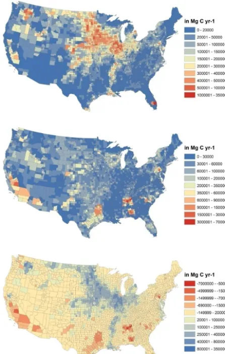
Figure 2. Spatial distributions of annual crop production (top); crop

consumption (middle); and crop NEP (bottom) for 2003. Data from CDIAC (2014).

oats, barley, wheat, sunflower, hay, sorghum, cotton, rice, peanuts, potatoes, sugar beets, sugarcane, tobacco, rye, and beans) representing the majority of the crops grown in the conterminous US (West et al., 2010, 2011). The harvested amount is calculated based on crop yields. Carbon released from biomass decomposition is calculated from NPP by sub-tracting the amount that is harvested. The remainder of crops, i.e., the amount not harvested, is left as residue and is either sequestered into the soil or decomposed within the same year. Changes in soil carbon are calculated based on empirical relationships between land management practices and soil carbon change (West et al., 2008). In order to capture the long-term impacts on soil carbon pools from a 20-year his-tory of changes in crop rotation and tillage intensity, the soil carbon change was calculated from 1980 to 2008.

3.1.2 Human and livestock consumption

Human crop carbon consumption data provided by West et al. (2011) were calculated based on the per capita food

con-sumption and the US population census data. The livestock consumption data were calculated in a similar way but also considered different feed consumption rates of different ani-mal species. The consumed amount was assumed to be re-leased back into the atmosphere within the same year as CO2 through respiration, excretion, and flatus (West et al.,

2009). Excretion typically entered the waste treatment facil-ities within the county, and the emissions were taken into account in the consumption term above.

3.2 Prior flux adjustments for US croplands

One way to integrate the carbon exchange of crops into the inversion model is to adjust the prior NEP modeled by BEPS. As part of the crop carbon exchange, the harvested amount is taken away from the field and respired back to the atmo-sphere when consumed by humans,Rhuman_consumption, and

livestock,Rlivestock_consumption. Therefore, crop NEP is given

by

NEPcrop=NPPcrop−Rh, residue−Rhuman_consumption −Rlivestock_consumption+1csoil. (12)

Since the residue amount, including both the remaining aboveground and belowground biomass, is the difference between the total crop biomass and the amount harvested, Eq. (12) can be rewritten as:

NEPcrop=NPPharvested+1csoil−Rhuman_consumption −Rlivestock_consumption=production-consumption, (13)

where

production=NPPharvested+1csoil, (14)

consumption=Rhuman_consumption

+Rlivestock_consumption. (15)

The spatial patterns of crop production, consumption, and NEP are shown in Fig. 2. The spatial distributions of crop production and consumption are calculated monthly and are used to adjust the monthly NEP distributions modeled by BEPS over the conterminous US. The production and con-sumption terms are adjusted separately due to their different seasonal patterns.

3.2.1 Production adjustment

The simulated terrestrial NPP by BEPS is adjusted to inte-grate cropland production over the contiguous US using the following equation:

NPPadjusted=NPPbiosphere−rcrop_area·(NPPbiosphere) +production=(1−rcrop_area)·NPPbiosphere +production=(1−rcrop_area)·NPPbiosphere

+NPPharvested+1csoil, (16)

where NPPbiosphereis the 1◦×1◦NPP output from BEPS and

grid over the total area of the grid. The county-level crop-land production is first extrapolated into a mean value for each 1◦_×1◦_{grid and then adjusted using Eq. (16). The ratio}

rcrop_areais calculated based on the harvested area data. The

basic idea of Eq. (16) is to replace BEPS NPP with more ac-curate crop production data for the portion of land area that is used for crop production, while BEPS NPP is unchanged for the remaining area. In this way, both the productive and non-productive areas in a grid are included in the prior, and the simulation of non-crop area by BEPS may be influenced by adjacent crop areas. BEPS uses GLC2000 as the land cover data in NPP simulations, but these data are not as accurate as the agricultural crop area statistics within each grid. Chan and Lin (2011) cautioned researchers against the direct com-parison of carbon accounting based on agricultural census data and fluxes simulated by biospheric models due to large differences of different land cover classifications used by the models. For this reason, we choose to use the crop area ratio method for the production adjustment.

Since the prior surface CO2 fluxes enter into the

atmo-spheric transport model on hourly time steps, the annual crop carbon production data are interpolated into the seasonal and diurnal patterns simulated by BEPS. Firstly, the annual NPPbiosphere is converted to annual NPPadjusted, and the

ra-tio between the two is taken and multiplied by the hourly NPPbiospherefluxes, resulting in hourly adjusted fluxes from

2000 to 2008 for each 1◦×1◦grid.

3.2.2 Consumption adjustment

The consumption terms are integrated into BEPS-simulated Rhover the contiguous US using the following equation:

Rh, adjusted=Rh, biosphere−rcrop_area·(Rh, biosphere) +consumption=(1−rcrop_area)·Rh, biosphere +consumption=(1−rcrop_area)·Rh, biosphere

+Rhuman_consumption+Rlivestock_consumption, (17)

whereRh, biosphere is the 1◦×1◦Rh output from BEPS and

rcrop_areais the ratio of harvested crop area within the 1◦×1◦

grid over the total area of the grid. The county-level crop-land consumption data are first resampled into each 1◦×1◦ grid, and the mean value of each grid is used to adjustRh

us-ing Eq. (17). However, unlike the production adjustment, the temporal patterns of CO2release from human and livestock

consumptions do not follow the seasonal and diurnal patterns simulated for the biosphere. We therefore assume constant hourly release of CO2from crop consumption throughout the

year. In this way, the annual consumption amount is divided equally into the hourly values and added to the hourly simu-latedRh, biospherefrom BEPS for the time period from 2000

to 2008 at each 1◦×1◦grid.

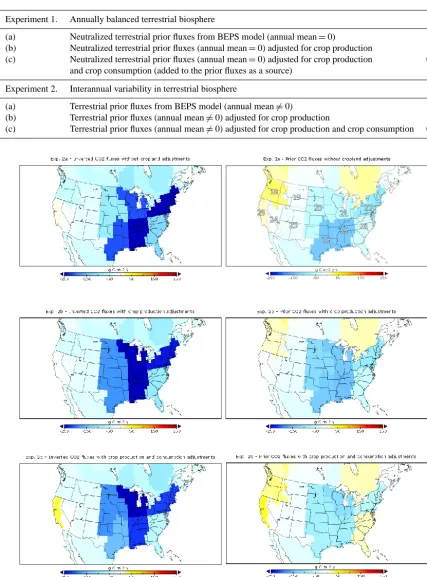
3.3 Schemes of inversion experiments

Two sets of inversion experiments (Table 2) are designed to test for the impact of integrating the cropland carbon data into the prior terrestrial flux. In the first set (Exper-iments 1a, 1b, 1c), the monthly terrestrial biosphere NEP modeled by BEPS at hourly time steps is first neutralized on an annual basis, meaning that the annual mean terrestrial flux is 0 for each grid cell but its seasonal variation is re-tained. The neutralized flux is then adjusted for crop produc-tion and consumpproduc-tion in Experiments 1b and 1c. After these adjustments, the annual prior flux in Experiments 1b and 1c (Table 3) differs from zero. The prior terrestrial surface flux in many atmospheric inversion studies only contains seasonal instead of interannual variations (Gurney, 2004; Rödenbeck et al., 2003) in order to minimize the influence of the errors in the prior flux on the inverted annual flux so that the results are mostly based on the “atmospheric view”. In the second set (Experiments 2a, 2b, 2c), the same monthly BEPS NEP is used without annual neutralization (Table 3) so that both seasonal and interannual variations in NEP are retained and the best estimate of the biospheric carbon flux is used to con-strain the inversion. Experiments 1a–c are therefore designed to explore the strength of the carbon cycle signal in the atmo-spheric CO2measurement, while Experiments 2a–c are

con-sidered to be the best final estimates by integrating ecosys-tem modeling results and crop statistics. In each set of exper-iments, there is a control run (Experiments 1a, 2a), which is used to assess influences of the production adjustment (Ex-periments 1b, 2b) and influences of the combined production and consumption adjustments (Experiments 1c, 2c) on the inverted flux.

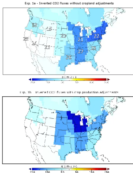
Figure 3. Map of mean annual inverted CO2flux for experiment 1

during 2002 to 2007 over contiguous US regions. Negative values represent carbon uptake.

4 Results and discussion

The inversion experiments described in Sect. 3.3 are con-ducted to test the impacts of cropland inventory on the in-verted CO2 fluxes. The impacts are evaluated based on the

multi-year mean annual values and seasonal variations. 4.1 Multi-year regional carbon budget

4.1.1 Average annual flux

The average annual inverted CO2fluxes over the

contermi-nous US are reported for experiment 1 (Fig. 3) and

experi-ment 2 (Fig. 4). Table 4 summarizes the mean inverted CO2

fluxes (µ)and errors (ε), as well as the percentage changes (1%) from the control case calculated by

1%=µ−µcontrol µcontrol

, (18)

whereµcontrolis the annual mean inverted flux for the

corre-sponding control experiment.

To evaluate the impact of integrating crop production and consumption data into the prior fluxes, comparisons of the inverted fluxes can be made between the experiments with and without crop adjustments. However, in order for these comparisons to be meaningful, a signal-to-noise ratio (SNR) is calculated for each region, using the following equation: SNR=|µ−µcontrol|

ε , (19)

whereεis the posterior uncertainty in the inverted flux for a region. Note that the “signal” is defined here as the mean difference in the inverted fluxes between the control and a crop-adjusted experiment, in order to represent the signal in-troduced by the adjustment. If SNR is less than unity, the re-sulting change due to an agricultural adjustment is less than the uncertainty, and hence the signal is within the noise level of the results. In Table 4, regions with SNR greater than unity are denoted with an asterisk.

Comparing Fig. 3a and b, it can be seen that the produc-tion adjustment redistributed the carbon sink from forested regions in the southeast (regions 26 to 28) and northwest (regions 18, 19) to cropland area in the Midwest (regions 20 and 21). SNR for experiment 1b for region 20 is greater than 1 (Table 4), indicating that the sink increase in this re-gion is beyond inversion uncertainty. The increase in the sink size in the US Midwest can be attributed to the large CO2

uptake during the growing season, but much of the carbon is released through crop consumption in other geographic locations. Seasonal results for these regions are shown in Sect. 4.1.3.

Canadian sink by 15 %, and the crop production and con-sumption adjustments (experiment 1c) reduce the sink by 1.4 and 12.1 % for USA and Canada, respectively, relative to the control case (experiment 1a, Table 4). These results suggest that the crop information used in the inversion affects not only US carbon sinks but also neighboring regions (such as Canada). The inverted results from both crop production and consumption adjustments (experiment 1c, Fig. 3c) show that the US Midwest sink in 2002–2007 is 425±129 Tg C yr−1. This sink value obtained in experiment 1c is smaller than that (522 Tg C yr−1)in experiment 1b but considerably larger than that (189 Tg C yr−1)in the control case, confirming the importance of considering the crop production and consump-tion data for atmospheric inversion.

Experiments 1a–c analyzed above are designed to accen-tuate the information content of atmospheric CO2

measure-ments for the surface carbon flux by neutralizing the annual biospheric flux before making the crop consumption adjust-ments. However, it could be argued that the annually neu-tralized fluxes may not be the best prior information for straining the inversion. Experiments 2a–c are therefore con-ducted with the best prior estimates possible based on a bio-spheric model and crop data. The prior biobio-spheric carbon flux used in experiment 2 differs from that in experiment 1 in the following ways: (1) the annual net carbon flux modeled by BEPS is used without neutralization, (2) the interannual vari-ations in the prior flux are considered, and (3) the interan-nual variations in crop production and consumption are also considered. Although errors in the annual mean prior fluxes would have imprints on the inverted results in experiment 2, the unneutralized fluxes may nudge the inverted results closer to reality as they integrate prior knowledge on the carbon source and sink distribution and the interannual variability.

Figure 4 shows inverted results under experiment 2 with comparisons to the prior estimates. The production adjust-ment (experiadjust-ment 2b) leads to significant increases in the CO2sink in the Midwest crop area (region 20). Regions 19,

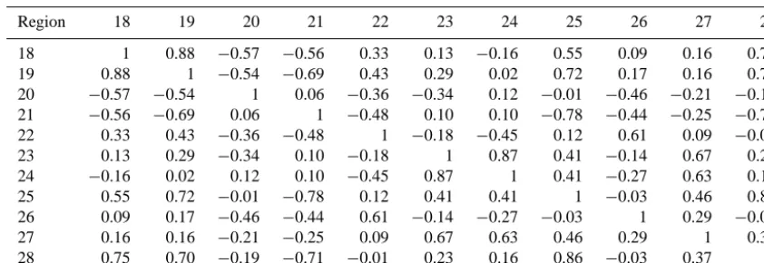
21, and 25 also gain noticeable sink increases, but sinks in other regions in the US decrease in compensation for these gains. Relative to experiment 2b, the additional consumption adjustment made in experiment 2c significantly weakened the sinks in the west region and noticeably in the southeast. These results are consistent with the findings from experi-ment 1. Crop adjustexperi-ments in experiexperi-ment 2 greatly enhanced the sinks in the cropland in the US Midwest (regions 20, 21), mostly at the expense of forested areas in the southeast (re-gions 26, 27, 28). This is also similar to experiment 1, which only takes into account the seasonal variations and not the in-terannual variations. For the purpose of comprehensive eval-uation of how crop adjustments spatially redistribute the car-bon flux, Table 5 provides a matrix of correlation coefficients of the change in the inverted flux from experiment 2a to ex-periment 2c among the 11 regions in the US, where positive correlations indicate that crop adjustments make the inverted flux increase or decrease in the same direction. Region 21,

for example, is negatively correlated with most regions ex-cept regions 20, 23, and 24, suggesting that its increase in carbon sink after the crop adjustments is mostly balanced by decreases in other regions except regions 20, 23, and 24. Another interesting example is region 28, which is strongly and negatively correlated with the Midwest region 21 and strongly and positively correlated to the west regions 18, 19, and 25. A large part of these correlations is due to adjust-ments to the priors (Table 3), as the change in the inverted flux for a region is highly correlated with the adjustment to the region (Fig. 6). However, atmospheric circulation pat-terns, such as the westerly and the monsoon air flows (air mass moving from the southeast to the Midwest), could also have impacts on these correlations.

Table 2. Schemes of experiments designed to test for the impact of integrating information from crop production and consumption data into

the prior fluxes.

Experiment 1. Annually balanced terrestrial biosphere χ2

(a) Neutralized terrestrial prior fluxes from BEPS model (annual mean=0) 1.09

(b) Neutralized terrestrial prior fluxes (annual mean=0) adjusted for crop production 1.12

(c) Neutralized terrestrial prior fluxes (annual mean=0) adjusted for crop production 0.97

and crop consumption (added to the prior fluxes as a source)

Experiment 2. Interannual variability in terrestrial biosphere χ2

(a) Terrestrial prior fluxes from BEPS model (annual mean6=0) 1.11

(b) Terrestrial prior fluxes (annual mean6=0) adjusted for crop production 1.16

(c) Terrestrial prior fluxes (annual mean6=0) adjusted for crop production and crop consumption 0.97

1

Figure 4. Map of mean annual inverted (left) and prior (right) CO2flux for experiment 2 during 2002 to 2007 over the contiguous US.

Table 3. Prior fluxes used in the two sets of inversion experiments

Region Experiment 1 Experiment 2

a b c a b c

18 0±6.5 −8.91±8.3 −1.94±9.5 15.88±6.5 6.97±8.3 13.94±9.5

19 0±2.9 −6.35±3.7 −1.96±4.4 −5.69±2.9 −12.04±3.7 −7.65±4.4

20 0±8.6 −75.83±27.4 −37.47±32.9 −66.51±8.6 −142.34±27.4 −103.98±32.9

21 0±8.5 −51.75±18.2 −34.97±20.3 −34.71±8.5 −86.46±18.2 −69.69±20.3

22 0±9.6 −0.42±11.6 17.56±13.6 −49.03±9.6 −49.45±11.6 −31.47±13.6

23 0±3.0 −1.93±3.9 5.38±6.2 2.75±3.0 0.82±3.9 8.12±6.2

24 0±0.7 −1.14±1.8 3.80±5.5 −2.95±0.7 −4.09±1.8 0.85±5.5

25 0±3.0 −3.97±3.8 3.39±5.1 −16.78±3.0 −20.75±3.8 −13.40±5.1

26 0±12.5 3.02±15.1 48.67±23.0 −105.11±12.5 −102.09±15.1 −56.45±23.0

27 0±14.9 −4.86±20.0 36.57±26.6 −88.63±14.9 −93.49±20.0 −52.06±26.6

28 0±15.6 −4.69±18.7 29.87±24.9 −21.50±15.6 −26.19±18.7 8.37±24.9

West 0±4.2 −22.29±5.4 8.66±7.2 −6.79±4.2 −29.09±5.4 1.86±7.2

Midwest 0±8.6 −127.56±23.3 −72.43±27.3 −101.22±8.6 −228.79±23.3 −173.66±27.3

Northeast 0±9.6 −0.35±11.6 17.56±13.6 −49.03±9.6 −49.45±11.6 −31.47±13.6

Southeast 0±14.3 −6.53±18.1 115.11±24.9 −215.24±14.3 −221.77±18.1 −100.14±24.9

US 0±9.9 −156.83±16.1 68.87±20.0 −372.28±9.9 −529.11±16.1 −303.41±20.0

Canada 0±5.9 0.00±5.9 0.00±5.9 50.75±5.9 50.75±5.9 50.75±5.9

NA 0±9.1 −156.83±14.8 68.87±18.5 −363.99±9.1 −520.81±14.8 −295.12±18.5

Table 4. Mean inverted CO₂flux (µ), error (ε)in Tg C yr−1,and the percentage change (1%) for global regions from 2002 to 2007.

Region Experiment 1 Experiment 2

(a) (b) (c) (a) (b) (c)

µ±ε µ±ε 1% µ±ε 1% µ±ε µ±ε 1% µ±ε 1%

18 −43.27±33.1 −38.45±25.7 −11.13 −30.41±28.4 −29.71 −26.48±33.1 −18.95±25.7 −28.43 −14.74±28.4 −44.32 19 −10.80±20.3 −17.94±15.8 66.08 −9.49±17.7 −12.07 −15.22±20.3 −17.18±15.8 12.88 −13.41±17.7 −11.87 20 −71.59±56.9 −271.27±91.4 278.94∗ −223.82±102.4 212.67∗ −113.85±56.9 −227.33±91.4 99.67∗ −231.71±102.4 103.52∗ 21 −117.07±59.8 −251.38±72.7 114.73∗ −201.33±78.3 71.98 −132.20±59.8 −192.76±72.7 45.81 −188.63±78.3 42.68 22 −104.91±57.7 −97.89±46.1 −6.69 −64.04±51.9 −38.95 −145.62±57.7 −124.70±46.1 −14.36 −113.33±51.9 −22.17 23 −0.79±8.9 −10.69±7 1257.11∗ 23.21±10.2 −3044.92∗ 1.66±8.9 0.34±7 −79.75 7.23±10.2 334.19 24 −0.05±0 −2.26±0 4169.81∗ 6.71±3.5 −12754.7∗ −3.00±0 −4.93±0 64.71∗ −0.12±3.5 −96.03 25 −7.95±14.2 −7.69±10.9 −3.29 −4.29±14.2 −45.94 −23.48±14.2 −26.09±10.9 11.12 −19.70±14.2 −16.1 26 −92.88±59.8 −79.49±47.5 −14.42 −36.65±63.8 −60.54 −160.95±59.8 −138.33±47.5 −14.06 −113.01±63.8 −29.79 27 −111.07±78.7 −76.22±64.6 −31.38 −63.91±82.9 −42.46 −175.18±78.7 −167.96±64.6 −4.12 −141.68±82.9 −19.12 28 −69.17±67.5 −52.21±51 −24.52 −16.86±64.5 −75.68 −76.25±67.5 −63.05±51 −17.3 −38.29±64.5 −49.78 West −62.85±39.1 −77.03±30.4 22.55 −14.29±32.7 −77.26∗ −66.50±40.2 −66.81±20.6 0.46 −40.75±23.4 −38.73∗ Midwest −188.65±80.7 −522.65±116.8 177.04∗ −425.15±128.8 125.36∗ −246.05±82.3 −420.09±115.5 70.73∗ −420.33±128.2 70.83∗ Northeast −104.91±57.7 −97.89±46.1 −6.69 −64.04±51.9 −38.95 −145.62±57.7 −124.70±46.1 −14.36 −131.31±51.9 −9.82 Southeast −273.13±118.2 −207.92±94.2 −23.87 −117.42±119.3 −57.01 −412.38±115.5 −369.34±93.1 −10.44 −292.98±119.4 −28.95 US −629.54±157.7 −905.48±153.9 43.83 −620.91±172.7 −1.37 −870.55±156.3 −980.94±152.2 12.68 −885.37±182.4 1.7 Canada −295.59±142.8 −340.58±139.5 −15.22 −259.87±139.7 −12.08 −255.50±137.2 −219.74±136.7 −14 −217.45±136.3 −14.89 NA −932.61±205.9 −1222.9±195.9 31.12 −883.58±211.4 −5.26 −1139.67±189.9 −1206.04±181.8 5.82 −1110.17±200.3 −2.59

∗_{Represents regions with SNR > 1, and positive percentage change in1% represents increase in uptake. West includes regions 18, 19, 23, 24, and 25; Midwest includes regions}

20 and 21; northeast includes region 22; and southeast includes regions 26, 27, and 28.

the atmospheric CO2measurements are able to differentiate

about two-third of the differences in fluxes among the regions and the inverted flux is highly sensitive to the prior flux.

Even though the nested regions in North America are fairly large, the atmospheric signal from the CO2observation

net-work is blurred substantially among the regions due to effi-cient atmospheric mixing. Schuh et al. (2010) conducted a high-resolution inversion over North America and found that the inverted flux spatial distribution in 40 km grids differs greatly from that of CarbonTracker because the prior fluxes

y = 1.5907x - 12.661 R² = 0.9171 -300 -250 -200 -150 -100 -50 0 50

-150 -100 -50 0 50

P os ter ior Fl ux of Ex p. 2 a (T gC/y)

Prior Flux of Exp. 2a (TgC/y)

y = 1.5793x - 12.483 R² = 0.9549 -50 -25 0 25 50 75 100 125 150

-50 -25 0 25 50 75 100

P os te ri or F lux Cha ng e of Ex p. 2c (T gC /y)

Prior Flux Adjust. of Exp. 2c (TgC/y)

y = 1.4224x + 2.5515 R² = 0.6348

-250 -200 -150 -100 -50 0 50

-150 -100 -50 0 50

P os te ri or F lux o f Ex p. 2c (T gC /y)

Posterior Flux of Exp. 1a (TgC/y)

y = 1.4003x + 0.999 R² = 0.9082

-250 -200 -150 -100 -50 0 50

-150 -100 -50 0 50

P os te ri or F lux of Ex p. 2a (T gC /y)

Posteiror Flux of Exp. 1a (TgC/g)

(d) (c)

(a) (b)

(c) (d)

Figure 5. Dependence of the posterior flux from inversions on

the prior flux for regions 18–28. (a) Correlation between posterior fluxes from experiment 2a and their prior fluxes, (b) correlation be-tween changes in posterior fluxes from experiment 2c and adjust-ments to their prior fluxes, (c) correlation of the posterior fluxes between experiment 1a and experiment 2c, and (d) correlation of the posterior fluxes between experiment 1a and experiment 2a.

scales smaller than 600 km. Our nested region size is about the same as this decorrelation distance, and therefore our in-verted regional fluxes do not lose much spatial information contained in the atmospheric measurements.

The result of experiment 2a for region 20 is comparable to the sink of 0.11 Pg C yr−1for cropland in about the same region from 2001 to 2005 reported by Peters et al. (2007), in which the biospheric flux was not adjusted for crop pro-duction and consumption. The comparison suggests that both sets of inversions captured about the same strength of the atmospheric sink signal in this region. After crop adjust-ments in experiment 2c, the sink magnitude in region 20 is approximately doubled with a total of 0.23 Pg C yr−1 (Ta-ble 4) or 298 g C m−2yr−1. The corresponding sink mag-nitude in region 21 is 0.19 Pg C yr−1 or 181 g C m−2yr−1. In the Mid-Continent Intensive (MCI) study (Schuh et al., 2013), three inversion models produced an average sink of about 0.15 Pg C yr−1or 150 g C m−2yr−1. This result is com-parable to the value of 0.183 Pg C yr−1or 183 g C m−2yr−1 produced in another inversion study (Lauvaux et al., 2012) for the same MCI area over a growing season from June to December (the dormant season in other months presumably has small fluxes). The MCI study area of 1000 km×1000 km covers 52 % of regions 20 and 21, with areas of 1275 and 631 km2, respectively. The area-weighted flux density of these two regions is 219 g C m−2yr−1, which is about 15– 40 % larger than previous inversion results from Schuh et al. (2013) and Lauvaux et al. (2012). The difference of our in-version results from these MCI studies is within the posterior uncertainty of our inversion, but it also indicates the need for further evaluation of our inversion results. In these regions,

the major crops are corn and soybean. Using eddy covariance systems at three local sites in region 20, Verma et al. (2005) measured NEP of irrigated corn, irrigated corn–soybean rota-tion, and rainfed corn–soybean rotation in 2001–2004 to be 441, 351, and 296 g C m−2yr−1, respectively. The inverted sink per unit land area is much smaller than these site-level sink values because productive crops only occupy about 50 % of the area in these regions.

Table 4 also provides aggregated results for four large US census regions – west, Midwest, northeast, and southeast – as well as the US and Canada. Crop consumption adjustments make significant (SNR > 1) changes to the inverted carbon flux in the west region in both experiments 1 and 2. This is mostly due to the large crop consumption in California. In experiment 2b with the non-neutralized and interannually variable prior biospheric flux, the crop production adjustment alone does not greatly affect the inverted sink in the west re-gion, but it does significantly increase the sink in the Midwest region with high crop production. Similar to experiment 1, the total sinks in North America and Canada from experi-ment 2 show large changes in sink sizes after the production adjustment. This suggests that in atmospheric inversion esti-mates the changes in the a priori flux affect the inverted re-sults not only locally but also globally (Gurney et al., 2004). The overall US and North American carbon sinks are similar to the control case when the crop consumption adjustment is also made (experiments 2b), where the percentage changes are only 1.7 and−2.6 % (Table 3), respectively. This result reinforces our original assumption that the long-term crop-land carbon budget is approximately balanced between the crop production and consumption (West et al., 2011). 4.1.2 Multi-year global carbon budget

Although the cropland carbon adjustments were only made for the US regions, the CO2 flux is inverted globally

us-ing the nested inversion system, which not only avoids the need to set up boundary conditions for North America but also produces results for other regions for comprehensive analysis. Table 6 provides the average annual inverted CO2

fluxes globally from 2002 to 2007 for experiments 1 and 2. It also summarizes the mean inverted CO2 fluxes (µ) and

errors (ε), as well as percentage changes (1%) from the control case for the large regions outside of North Amer-ica. In the results for both experiments 1 and 2, agricultural adjustments affect the two North America regions (NA-S and NA-N) similarly, indicating that these two regions are closely linked as many CO2stations within and around North

Table 5. Correlation coefficients of the change in the inverted flux from experiments 2a to that of experiment 2c among 11 regions in the US,

calculated based on inverted annual fluxes in 2000–2007.

Region 18 19 20 21 22 23 24 25 26 27 28

18 1 0.88 −0.57 −0.56 0.33 0.13 −0.16 0.55 0.09 0.16 0.75

19 0.88 1 −0.54 −0.69 0.43 0.29 0.02 0.72 0.17 0.16 0.70

20 −0.57 −0.54 1 0.06 −0.36 −0.34 0.12 −0.01 −0.46 −0.21 −0.19

21 −0.56 −0.69 0.06 1 −0.48 0.10 0.10 −0.78 −0.44 −0.25 −0.71

22 0.33 0.43 −0.36 −0.48 1 −0.18 −0.45 0.12 0.61 0.09 −0.01

23 0.13 0.29 −0.34 0.10 −0.18 1 0.87 0.41 −0.14 0.67 0.23

24 −0.16 0.02 0.12 0.10 −0.45 0.87 1 0.41 −0.27 0.63 0.16

25 0.55 0.72 −0.01 −0.78 0.12 0.41 0.41 1 −0.03 0.46 0.86

26 0.09 0.17 −0.46 −0.44 0.61 −0.14 −0.27 −0.03 1 0.29 −0.03

27 0.16 0.16 −0.21 −0.25 0.09 0.67 0.63 0.46 0.29 1 0.37

28 0.75 0.70 −0.19 −0.71 −0.01 0.23 0.16 0.86 −0.03 0.37 1

budget is constrained by mean changes in the atmospheric CO2concentration. In an atmospheric inversion study,

Gur-ney et al. (2004) found that contributions from land fluxes ap-peared in the adjacent ocean regions, and they described this phenomenon as flux “leakage”. In our case, the compensat-ing effect seen in other regions outside of the conterminous US may also be considered as a leakage. This leakage puts into question the reliability of the atmospheric CO2

measure-ments in optimizing the local flux if the prior information is biased, given the fact that North America is one of the conti-nents with strong data constraints. We would therefore expect that similar adjustments in other regions of the globe with fewer observation stations can cause larger flux leakages to-ward regions with weaker atmospheric constraints.

The inverted total global land sink from experiment 2 is larger than that from experiment 1 (Table 5) because the prior land sink in experiment 2 is larger than that in experiment 1. To compensate for this influence of the prior flux over land, the inverted ocean sink is smaller in experiment 2 than in experiment 1. The total land and ocean sinks do not show large changes with the crop production or crop consumption adjustments in the US in both experiments (Table 5). Rel-ative to experiment 1, experiment 2 shows a slightly larger decrease in the terrestrial sink and a slightly larger increase in the ocean sink. The overall crop adjustments allocate a slightly smaller sink to North America, while most regions outside of North America adjust accordingly to balance the global carbon budget due to weak data constraints in other regions.

4.1.3 Seasonal variation

The timing of the CO2 uptake and release from croplands

exerts great influences on the atmospheric CO2 (Corbin et

al., 2010), as crops in different regions differ in their growth patterns. The seasonal variation pattern in the surface flux may coincide with that in the strength of atmospheric bound-ary layer mixing, causing the rectifier effect on atmospheric

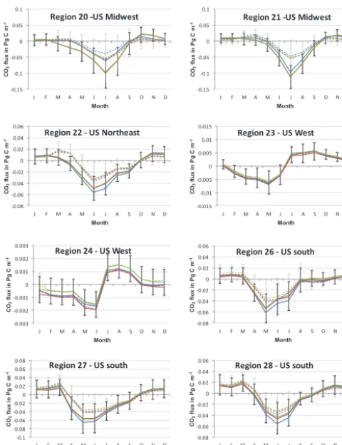
transport (Denning et al., 1995; Gurney, 2004). In this re-search, the a priori seasonal variation for cropland is based on BEPS, which considers the seasonal variations in vegeta-tion structure using remotely sensed LAI and meteorology. Figure 6 shows the monthly a priori and a posteriori CO2

fluxes for the period of 2002–2007 from experiment 2 for re-gions of high crop production and high crop consumption in the US. Results from experiment 1 are not shown, but they are similar in the seasonal variation pattern.

In regions 20 and 21 of high crop production, the inverted monthly fluxes with agricultural adjustments show higher up-take during the peak growing season of June, July, and Au-gust and a stronger release of carbon during the non-growing season in October and November than the prior fluxes. March and April show a net uptake in the CO2 inverted fluxes in

agriculturally adjusted experiments in region 20 instead of near carbon neutrality shown in the control experiment. In regions 23 and 24 of high crop consumption with low vegeta-tion, the impacts of crop consumption adjustment are mostly shown as persistent decreases in sinks throughout the year, while those with the production adjustment have persistent increases. In the US southeast, a region with mixed forests and moderate crop production and consumption (regions 26, 27, 28), the crop production adjustment (experiment 2b) and the crop production and consumption adjustments (experi-ment 2c) cause discernible to considerable impacts on the magnitude of the CO2uptake during the growing season and

release during non-growing seasons.

The changes in the monthly inverted fluxes after adjust-ing for crop production and consumption are mainly ob-served as changes in the magnitude instead of the timing of the growing seasons. This means that the seasonal pat-tern of the inverted CO2flux generally follows that of the a

-0.15 -0.1 -0.05 0 0.05 0.1

J F M A M J J A S O N D CO2 flux in P g C m -1 Month Region 20 -US Midwest

-0.15 -0.1 -0.05 0 0.05 0.1

J F M A M J J A S O N D

CO 2 flux in P g C m -1 Month Region 21 -US Midwest

-0.08 -0.06 -0.04 -0.02 0 0.02 0.04 0.06

J F M A M J J A S O N D

CO 2 flux in P g C m -1 Month Region 22 - US Northeast

-0.015 -0.01 -0.005 0 0.005 0.01 0.015

J F M A M J J A S O N D CO2 flux in P g C m -1 Month Region 23 - US West

-0.003 -0.002 -0.001 0 0.001 0.002 0.003

J F M A M J J A S O N D CO2 flux in P g C m -1 Month Region 24 - US West

-0.08 -0.06 -0.04 -0.02 0 0.02 0.04 0.06

J F M A M J J A S O N D CO2 flux in P g C m -1 Month Region 26 - US south

-0.1 -0.08 -0.06 -0.04 -0.02 0 0.02 0.04 0.06 0.08

J F M A M J J A S O N D CO2 flux in P g C m -1 Month Region 27 - US south

-0.08 -0.06 -0.04 -0.02 0 0.02 0.04 0.06

J F M A M J J A S O N D

CO 2 flux in P g C m -1 Month Region 28 - US south

Figure 6. Monthly inverted (solid lines) and prior (dashed lines)

CO2flux (negative values are sinks) averaged over 2002 to 2007

for Experiments 2 – annually varying terrestrial prior fluxes with

(a) no adjustments – blue; (b) production adjustments – red; (c) crop

production and consumption adjustments – green.

information, although they are also subject to certain uncer-tainties due to errors in retrieved LAI and the model. 4.2 Discussion

After integrating US crop production and consumption data into the prior flux, the US Midwest becomes a large regional CO2sink from 2002 to 2007 in our inverse modeling. This

is mainly due to the large uptake of CO2 during the

grow-ing season (Peters et al., 2007). Because of the release of the CO2in regions of sizable crop consumption by humans

and livestock, a weakening of the US southeast forest sink is found in our inversion. With the neutralization of the an-nual prior flux before adjusting for crop consumption (exper-iment 1), the US Midwest is perceived by the “atmospheric view” as the dominant sink in North America. While crop-lands in the US Midwest uptake large amounts of carbon during the growing season, some of this carbon is decom-posed on-site, while the remainder is transported off-site and respired back to the atmosphere elsewhere. Therefore, lateral transport of carbon needs to be considered in order to rec-oncile atmospheric inversion results with ground-based

mea-surements (Hayes et al., 2012; Gourdji et al., 2012). On the west coast, including California, where there are high levels of human and livestock consumption, an overall CO2source

is obtained from the inversion. With the incorporation of US cropland carbon data, the main US sink is redistributed from the US southeast and west forested regions to the US Mid-west cropland in the inversion process. In order to assess the possible range of errors in our inversion system, this redistri-bution is shown in the results from two sets of experiments. Experiment 1, which gives larger weights to the influence of atmospheric CO2observation than to the prior terrestrial

flux, shows the sink in the US Midwest to be larger than that in the US southeast. Similar results are also obtained in ex-periment 2, which gives larger weights to the prior terrestrial flux as an opposite case. In both experiments, the inclusion of agricultural inventory data in the priors significantly al-tered the inversion results for several regions in the west and Midwest regions. Although the atmospheric CO2

measure-ments contain much information on the spatial distribution of the carbon sink over the continent, our analysis reveals that they are insufficient for differentiating large flux differences among productive and non-productive regions (Fig. 5). The inverted flux distribution is mostly determined by the prior distribution. This point may be no better demonstrated than the MCI study of Schuh et al. (2013), in which three inver-sion studies show different inverinver-sion results but all closely resemble the prior distributions, although there are 16 CO2

observation sites within the MCI study region.

In experiment 1, based on an annually neutralized prior ecosystem flux, the overall magnitudes of the US and North American sinks are weakened by∼1.4 and∼5.3 % after the cropland production and consumption adjustments are made, respectively. Furthermore, regions outside of the US are also affected by these adjustments, and the Canadian carbon sink shows noticeable weakening (12.1 %) (Table 4). Many re-gions outside of North America, which are not as well con-strained by CO2observations, also show small changes when

these adjustments are made (Table 6). While these changes may have been affected by the additional errors introduced to the uncertainty matrix of the prior flux, the leakage of the CO2 flux from the adjusted regions into other regions with

poor constraints may be the main reason for these changes (Gurney et al., 2004). While not conclusive, this phenomenon of leakage points to the importance of the prior flux for con-straining atmospheric inversion for the carbon flux of small regions with sparse atmospheric CO2measurements. Since

the unneutralized flux is closer to reality than the neutral-ized flux in terms of the annual sink magnitude, the following further discussion is therefore based on results from experi-ment 2.

Table 6. Mean inverted CO2flux (µ), error (ε)in Pg C yr−1, and the percentage change (1%) for global regions from 2002 to 2007.

Region Experiment 1 Experiment 2

(a) (b) (c) (a) (b) (c)

µ±ε µ±ε 1% µ±ε 1% µ±ε µ±ε 1% µ±ε 1%

NA-N −0.28±0.14 −0.24±0.14 −13.01 −0.26±0.14 −7.57 −0.22±0.14 −0.18±0.14 −14.89 −0.20±0.14 −7.83 NA-S −0.65±0.16 −0.74±0.16 14.07 −0.63±0.16 −2.95 −0.92±0.16 −1.02±0.16 10.65 −0.91±0.19 −1.37 31 0.36±0.41 0.35±0.41 −0.61 0.34±0.41 −5.59 0.34±0.41 0.39±0.41 14.34 0.37±0.41 9.12 32 −0.07±0.27 −0.07±0.27 −3.62 −0.06±0.27 −10.04 −0.11±0.27 −0.09±0.27 −16.89 −0.08±0.27 −21.02 33 −0.20±0.28 −0.19±0.28 −5.45 −0.22±0.28 8.30 −0.28±0.28 −0.19±0.28 −33.92 −0.22±0.28 −24.07 34 −0.86±0.27 −0.86±0.27 −0.15 −0.86±0.27 −0.63 −0.93±0.27 −0.91±0.27 −2.33 −0.91±0.27 −2.78 35 −0.90±0.26 −0.87±0.26 −2.97 −0.89±0.26 −0.40 −1.00±0.26 −0.96±0.26 −3.73 −0.99±0.26 −1.42 36 −0.63±0.24 −0.61±0.24 −3.34 −0.64±0.24 0.57 −0.52±0.24 −0.54±0.24 4.97 −0.57±0.24 9.75 37 −0.54±0.24 −0.54±0.24 0.57 −0.54±0.24 0.78 −0.63±0.24 −0.59±0.24 −7.49 −0.59±0.24 −7.32 38 0.06±0.08 0.06±0.08 1.05 0.06±0.08 1.91 0.04±0.08 0.04±0.08 −2.77 0.04±0.08 −1.58 39 −0.21±0.21 −0.18±0.21 −14.44 −0.19±0.21 −7.45 −0.06±0.21 −0.01±0.21 −88.22 −0.02±0.21 −64.84 40 −0.58±0.15 −0.58±0.15 1.22 −0.59±0.15 3.00 −0.62±0.15 −0.63±0.15 1.22 −0.64±0.15 2.87 41 −0.06±0.12 −0.07±0.12 10.86 −0.06±0.12 2.11 0.00±0.12 −0.01±0.12 138.30 0.00±0.12 −45.39 42 0.74±0.14 0.74±0.14 −0.72 0.74±0.14 −0.14 0.80±0.14 0.79±0.14 −0.90 0.79±0.14 −0.36 43 −0.58±0.18 −0.58±0.18 0.25 −0.58±0.18 −0.35 −0.51±0.18 −0.51±0.18 0.77 −0.51±0.18 0.08 44 −0.27±0.07 −0.28±0.07 2.85 −0.27±0.07 1.07 −0.27±0.07 −0.28±0.07 3.52 −0.28±0.07 1.76 45 −0.34±0.12 −0.34±0.12 −0.84 −0.36±0.12 4.30 −0.31±0.12 −0.30±0.12 −3.08 −0.32±0.12 2.52 46 0.10±0.12 0.10±0.12 −0.60 0.10±0.12 −0.41 0.15±0.12 0.15±0.12 1.02 0.15±0.12 1.14 47 −0.32±0.14 −0.32±0.14 −1.28 −0.32±0.14 −1.52 −0.33±0.14 −0.33±0.14 −0.94 −0.33±0.14 −1.18 48 0.15±0.06 0.15±0.06 −1.04 0.15±0.06 −0.77 0.14±0.06 0.14±0.06 −0.73 0.14±0.06 −0.45 49 0.06±0.16 0.05±0.16 −6.59 0.06±0.16 −2.21 0.14±0.16 0.14±0.16 2.54 0.15±0.16 4.36 50 −0.56±0.13 −0.56±0.13 −0.64 −0.56±0.13 −0.87 −0.53±0.13 −0.53±0.13 −0.42 −0.53±0.13 −0.66 Land −3.93±0.67 −3.89±0.67 −0.83 −3.90±0.65 −0.72 −4.30±0.66 −4.07±0.65 −5.39 −4.07±0.66 −5.29 Oceans −1.67±0.37 −1.69±0.37 1.43 −1.70±0.37 1.70 −1.37±0.38 −1.38±0.37 0.98 −1.39±0.37 1.31 Total −5.59±0.75 −5.59±0.75 −0.16 −5.59±0.74 0.01 −5.66±0.75 −5.45±0.74 −3.85 −5.46±0.75 −3.70

∗_{represents regions with SNR > 1, and positive percentage change in1% represents increase in uptake/release.}

the value of 0.047 Pg C yr−1for the net US agricultural car-bon export in 2008 estimated by West et al. (2011). For the US Midwest, the inverted results with agricultural adjust-ments show a large sink of 0.42±0.13 Pg C yr−1 (experi-ment 2c). The value is reduced to 0.24 Pg C yr−1if these ad-justments are not made (experiment 2a). These adad-justments make a difference of approximately 67 % of the total annual crop production in the US. This suggests that the NEP sim-ulations from the Boreal Ecosystem Productivity Simulator underestimate the processes that relate to cropland CO2sinks

because it assumes the consumption (respiration) occurs at the same location as production.

The US west and southeast, being regions of large population and crop consumption, show a combined 0.145 Pg C yr−1weakening of the sink after the crop adjust-ments (experiment 2c). This sink reduction is about 60 % of the total annual crop consumption averaged over 2002 to 2007 (∼0.24 Pg C yr−1, based on West et al., 2011), indicat-ing the importance of usindicat-ing the crop consumption data for these two regions in the inversion.

Using an atmospheric inversion technique over North America, Peters et al. (2007) showed the US Midwest to be the major sink and the US southeast forest region to be ei-ther carbon-neutral or a source between 2002 and 2007. In our inversion constrained by the annually neutralized a priori

flux adjusted for crop production and consumption (exper-iment 1c, Table 4), the US Midwest is also shown to be a large CO2sink, but the US southeast forest region remains