A Steady-state and Generational Evolutionary
Algorithm for Dynamic Multiobjective Optimization
Shouyong Jiang and Shengxiang Yang,
Senior Member, IEEE
Abstract—This paper presents a new algorithm, called steady-state and generational evolutionary algorithm, which combines the fast and steadily tracking ability of steady-state algorithms and good diversity preservation of generational algorithms, for handling dynamic multiobjective optimization. Unlike most existing approaches for dynamic multiobjective optimization, the proposed algorithm detects environmental changes and responds to them in a steady-state manner. If a change is detected, it reuses a portion of outdated solutions with good distribution and relocates a number of solutions close to the new Pareto front based on the information collected from previous environments and the new environment. This way, the algorithm can quickly adapt to changing environments and thus is expected to provide a good tracking ability. The proposed algorithm is tested on a number of bi- and three-objective benchmark problems with different dynamic characteristics and difficulties. Experimental results show that the proposed algorithm is very competitive for dynamic multiobjective optimization in comparison with state-of-the-art methods.
Index Terms—Steady-state and generational evolutionary al-gorithm, dynamic multiobjective optimization, change detection, change response.
I. INTRODUCTION
M
ANY real-world multiobjective optimization problems (MOPs) are dynamic in nature, whose objective func-tions, constraints, and/or parameters may change over time. Due to the presence of dynamisms, dynamic MOPs (DMOPs) pose big challenges to evolutionary algorithms (EAs) since any environmental change may affect the objective vector, constraints, and/or parameters. As a result, the Pareto-optimal set (POS), which is a set of mathematical solutions to MOPs, and/or the Pareto-optimal front (POF) that is the image of POS in the objective space, may change over time. Then, the optimization goal is to track the moving POF and/or POS and obtain a sequence of approximations over time.DMOPs can be defined in different ways, according to the nature of dynamisms [15], [41], [54]. In this paper, we mainly Manuscript received November 13, 2015; revised March 7, 2016 and May 3, 2016; accepted May 10, 2016. This work was supported by the Engineering and Physical Sciences Research Council (EPSRC) of UK under Grant EP/K001310/1 (Corresponding author: Shengxiang Yang).
The authors are with the Centre for Computational Intelligence (CCI), School of Computer Science and Informatics, De Montfort Univer-sity, Leicester LE1 9BH, U.K. (email: [email protected], [email protected]).
This paper has supplementary downloadable material provided by the au-thors, which is available at http://ieeexplore.org. This supplementary material provides the formulation of the test problems used in the paper and some supplementary experimental results. This material is 102 KB in size.
Copyright (c) 2012 IEEE. Personal use of this material is permitted. However, permission to use this material for any other purposes must be obtained from the IEEE by sending a request to [email protected].
consider the following kind of DMOPs:
min F(x, t) = (f1(x, t), ..., fM(x, t))T s.t. hi(x, t) = 0, i= 1, ..., nh gi(x, t)≥0, i= 1, ..., ng x∈Ωx, t∈Ωt (1)
where M is the number of objectives, nh and ng are the
number of equality and inequality constraints, respectively,
Ωx⊆Rnis the decision space,tis the discrete time instance, Ωt⊆Ris the time space, andF(x, t):Ωx×Ωt→RM is the
objective function vector that evaluates solutionxat timet. In the past few years, there has been an increasing amount of research interest in the field of evolutionary multiobjective optimization (EMO) as many real-world applications, like thermal scheduling [42] and circular antenna design [3], have at least two objectives that conflict with each other, i.e., they are MOPs. Due to multiobjectivity, the goal of solving MOPs is not to find a single optimal solution but to find a set of trade-off solutions. When an MOP involves time-dependent components, it can be regarded as a DMOP. Many real-life problems in nature are DMOPs, such as planning [8], scheduling [12], [35], and control [15], [50]. There have been a number of contributions made to several important aspects of this field, including dynamism classification [15], [41], test problems [4], [15], [20], [23]–[26], performance metrics [9], [15], [17]–[19], [41], [55], and algorithm design [9], [12], [15], [18], [21], [28], [54], [55]. Among these, algorithm design is the most important issue as it is the problem-solving tool for DMOPs.
Due to the presence of dynamisms, the design of a dynamic multiobjective optimization EA (DMOEA) is different from that of a multiobjective optimization EA (MOEA) for static MOPs. Specifically, DMOEAs should not only have a fast convergence performance (which is crucial to their tracking ability), but also be able to address diversity loss whenever there is an environmental change in order to explore the new search space. Besides, if changes are not assumed to be knowable, DMOEAs should be able to detect them in order not to mislead the optimization process. This is because, when a change occurs, the previously discovered POS may not remain optimal for the new environment.
In principle, a change can be detected by re-evaluating dedicated detectors [12], [18], [47], [54], [55] or assessing algorithm behaviours [15], [32], [37]. The former is a easy-to-use mechanism and allows “robust detection” [37] if a high enough number of detectors is used, but it may require additional cost since detectors have to be re-evaluated at every
generation, and it may not be accurate when there is noise in function evaluations. The latter does not need additional function evaluations, but it may cause false positives and thus make algorithms overreacting when no change occurs. Both of them cannot guarantee that changes are detected [37].
On the other hand, whenever a change is detected, it is often inefficient to restart the optimization process from scratch, although the restart strategy may be a good choice if the environmental change is considerably severe [7]. In the literature, various approaches have been proposed to handle environmental changes, and they can be mainly categorized into diversity-based approaches and convergence-based ap-proaches, according to their algorithm behaviours. Diversity-based approaches focus on maintaining population diversity whereas convergence-based ones aim to achieve a fast con-vergence performance so that algorithms’ tracking ability are guaranteed. Generally, population diversity can be handled by increasing diversity using mutation of selected old solutions or random generation of some new solutions upon the detec-tion of environmental changes [12], [18], [55], maintaining diversity throughout the optimization process [1], [2], [6], or employing multi-population schemes [18], [40]. Proper diversity is helpful for exploring promising search regions, but too much diversity may cause evolutionary stagnation [5]. Convergence-based approaches try to exploit past infor-mation for better tracking performance [7], especially when the new POS is somewhat similar to the previous one or environmental changes exhibit regular patterns. Accordingly, recording relevant past information to be reused at a later stage may be helpful for tracking the new POF as quickly as possible. The reuse of past information is closely related to the type of environmental change and hence can be helpful for different purposes [6]. If the environment changes periodically, relevant information of the current POS can be stored in a memory and can be directly re-introduced into the evolving population when needed. This kind of strategy is often called memory-based approaches and has been extensively studied in dynamic multiobjective optimization [7], [8], [18], [22], [52]. In contrast, if the environment change follows a regular pat-tern, past information can be collected and used to model the movement of the changing POF/POS. Hence, the location of the new POS can be predicted, helping the population quickly track the moving POF. Prediction-based approaches have received massive attention because most existing benchmark DMOPs (e.g., the FDA test suite [15]) involve predictable characteristics, and studies along this direction can be referred to [22], [28], [32], [33], [36], [47], [54], [55].
Aside from the above-mentioned approaches, some studies concentrate on finding an insensitive robust POF instead of closely tracking the moving POF [16], [27], [38]. Robustness-based approaches assume that when the environment changes, the old obtained solution can still be used in the new environ-ment as long as its quality is acceptable [27]. However, the criterion for an acceptable optimal solution is quite problem-specific, which may hinder the wide application of these approaches.
Although a number of approaches have been proposed for solving DMOPs, the development of DMOEAs is a relatively
Algorithm 1 Framework of SGEA 1: Input:N (population size)
2: Output: a series of approximated POFs
3: Create an initial parent populationP:={x1, . . . , xN}; 4: (A, P) :=EnvironmentSelection(P);
5: whilestopping criterion not metdo 6: fori:= 1toN do
7: ifchange detected and not respondedthen 8: ChangeResponse(); 9: end if 10: y:=GenerateOffspring(P, A); 11: (P, A) :=UpdatePopulation(y); 12: end for 13: (A, P) :=EnvironmentSelection(P∪P); 14: SetP:=P; 15: end while
young field and more studies are greatly needed. In this paper, a new algorithm, called steady-state and generational EA (SGEA), is proposed for efficiently handling DMOPs. SGEA makes most of the advantages of steady-state EAs in dynamic environments [48] for environmental change de-tection and response. If a change is detected, SGEA reuses a portion of old solutions with good diversity and exploits information collected from both previous environments and the new environment to relocate a part of its evolving population. At the end of every generation, like conventional generational EAs [13], [56], SGEA performs environmental selection to preserve good individuals for the next generation. By mixing the steady-state and generational manners, SGEA can adapt to dynamic environments quickly whenever a change occurs, providing very promising tracking ability for DMOPs.
The rest of this paper is organized as follows. Section II describes the framework of the proposed SGEA, together with detailed descriptions of each component of the algorithm. Section III is devoted to presenting experimental settings for comparison. Section IV provides experimental results and comparison on tested algorithms. A further discussion of the algorithm is offered in Section V. Section VI concludes the paper with discussions on future work.
II. PROPOSEDSGEA
The basic framework of the proposed SGEA is presented in Algorithm 1. SGEA starts with an initial populationP and the initialization of an elitist populationP and an archiveA through environmental selection. In every generational cycle, SGEA detects possible environmental changes and evolves the population in a steady-state manner. For each population member, if a change is detected, then a change response mech-anism is adopted to handle the detected change. After that, genetic operation is applied to produce one offspring solution for the population member, which is then used to update the parent population P and archive A. At the end of each generation, P and P are combined. Similar to generational EAs [13], [56] or speciation techniques used in niching [5], [29], a generational environmental selection is conducted on the combined population to preserve a population of good solutions for the next generation. This way, SGEA can be regarded as a steady-state and generational MOEA. In the
Algorithm 2 EnvironmentSelection(Q)
1: Input:Q(a set of solutions)
2: Output:A(archive),P (N elitists preserved)
3: SetA:=∅andP:=∅;
4: Assign a fitness value to each member inQ;
5: fori:= 1to|Q|do 6: ifF(i)<1then 7: CopyxifromQtoA; 8: end if 9: end for 10: if|A|< N then
11: Copy the best N individuals in terms of their fitness values fromQtoP;
12: else
13: if|A|==N then 14: SetP :=A;
15: else
16: PruneAto a set ofNindividuals by any truncation operator and copy the truncatedAtoP;
17: end if 18: end if
following subsections, the implementation of each component of SGEA will be detailed step by step.
A. Environmental Selection
The environmental selection procedure (Algorithm 2), which aims to preserve a fixed number of elitists from a solution setQafter every generational cycle, starts with fitness assignment. Each individualiofQis assigned a fitness value F(i), which is defined as the number of individuals that dominate [56] it, as follows:
F(i) =|{j∈Q|j≺i}| (2) where| · |denotes the cardinality of a set andj≺iindicates thatjdominatesi. It should be noted that, various fine-grained methods proposed in the literature [14], [45], [56] can be used to assign fitness values for individuals. However, the fitness assignment method used in this paper is relatively simple and computationally efficient. Most importantly, when an external individualeenters the setQ, the update ofF(i)needs only one dominance comparison between individualseandi. The easy-to-update property of this method will be clearly embodied in the population update procedure (to be described in Section II-C).
Afterwards, individuals having a fitness value of zero are identified as nondominated solutions and then copied to an archiveA. If|A|is smaller than the population sizeN, the best N individuals (including both dominated and nondominated ones) in terms of their fitness values are preserved in an elitist populationP. Otherwise, there can be two situations: either the number of nondominated solutions fits exactly the population size, or there are too many nondominated solutions. In the first case, all nondominated solutions are copied to P. In the second case, a truncation technique is needed to reduce A to a population of N nondominated solutions such that the truncated A have the best diversity possible. In SGEA, the k-th nearest neighbour truncation technique proposed in the strength Pareto EA 2 (SPEA2) [56] is used to perform the
Algorithm 3 GenerateOffspring(P, A)
1: Input:P (parent population),A(archive population)
2: Output:y(offspring solution)
3: ifrnd <0.5then
4: Perform binary tournament selection on P to select two distinct individuals as the mating parents;
5: else
6: Randomly pick an individual from A and perform binary tournament selection onPto select another distinct individual as the mating parents.
7: end if
8: Apply genetic operators to generate a new solutiony;
truncation operation, although we recognise there are other options, e.g., the farthest first method [10], [11], which can also serve this purpose. After that, solutions in the truncated Aare copied to P.
Note that, like classical generational MOEAs, such as the nondominated sorting genetic algorithm II (NSGA-II) [13] and SPEA2 [56], SGEA performs environmental selection at the end of each generation. Thus, SGEA can be generally categorized into generational MOEAs.
B. Mating Selection and Genetic Operators
Mating selection is an important operation before the pro-duction of new offspring (line 10 of Algorithm 1). In this paper, mating parents can be selected either from the parent populationP or the archive populationA. The benefit of such a mating selection method has been extensively investigated on static MOPs in a number of studies [30], [34], [44], [57]. While selecting mating parents fromP can maintain good population diversity, selecting parents from A can significantly improve the convergence speed of the population, which is considerably desirable in fast-changing environments. If a mating parent is to be selected fromP, SGEA performs a binary tournament selection according to individuals’ fitness values. If not, the mating parent can be randomly selected from the archive populationA.
Following the mating selection, genetic operators are ap-plied on the mating parents to generate a new offspring solu-tion. In SGEA, the simulation binary crossover and polynomial mutation are chosen as the recombination and mutation oper-ators, respectively. The reproduction procedure is presented in Algorithm 3.
C. Population Update
In SGEA, population update (line 11 of Algorithm 1) is conducted on both the parent population P and archive population A, which is detailed in Algorithm 4. The update operation onPis in fact replacing the worst solution ofPwith the newly generated solutionywhile the update onAis using y to update the archived nondominated set. First, ify is not a duplicate solution, it will be compared with each memberxi
ofP for the dominance relation (lines 4 to 14 of Algorithm 4). Ifydominatesxi(denoted asy≺xi), the fitness value ofxiis
increased by one. Ifyis dominated byxi(denoted asy≻xi),
Algorithm 4 UpdatePopulation(y)
1: Input:y(offspring solution)
2: Output: P (updated parent population), A (updated archive population)
3: Set the fitness value ofyas zero:F(y) := 0;
4: fori:= 1to|P|do 5: ify==xi then
6: Return;
7: end if 8: ify≺xithen
9: Add one to the fitness value ofxi:F(i) :=F(i) + 1; 10: end if
11: ify≻xithen
12: Add one to the fitness value ofy:F(y) :=F(y) + 1;
13: end if 14: end for
15: Compute the individual in P having the highest fitness value:
ˆi:=i:argmax{1≤i≤|P|}F(i); 16: ifF(y)≤F(ˆi)then
17: Setxˆi:=yandF(ˆi) :=F(y); 18: ifF(y)<1then
19: Remove all solutions in A that are dominated by y, and addytoA ifAis not full;
20: end if 21: end if
individual in P with the highest fitness value is identified, and if there are two or more such individuals, a random one is selected. If y is not worse than the identified individual xˆi in terms of the fitness value, the solution replacement takes place, as shown in line 17 of Algorithm 4. Besides, ifyis not dominated by any member inP (which means its fitness value is zero), it should be further considered to update the archive population AifA is not full. This means, the archive update occurs only wheny successfully enters the parent population. It can be observed that, the fitness assignment method used here is easy to update an individual’s fitness value, which helps SGEA conduct solution replacement in the parent population and archive update in an efficient manner.
D. Dynamism Handling
This section discusses two main aspects of dynamism handling. One is change detection, a step to detect whether a change has occurs during the evolutionary process. The other is known as change response or change reaction, which takes actions to quickly react to environmental changes so that the population adapts to new environments rapidly.
1) Change Detection: Change detection can be performed by either re-evaluating a portion of existing solutions [12], [18], [47], [54], [55] or assessing some statistical information of some selected population members [15], [32], [37]. Since both methods choose a small proportion of population mem-bers as detectors, detection may fail if changes occur on non-detectors. On the contrary, it will be computationally expensive if the whole population members are chosen as detectors. Therefore, a good detection method should strike a balance between the detection ability and efficiency.
The proposed algorithm detects changes in a steady-state manner, as shown in line 7 of Algorithm 1. In every generation, population members (in random order) are checked one by
one for discrepancy between their previous objective values and re-evaluated ones. If a discrepancy exists in a population member, we assume a change is successfully detected and there is no need to do further checks for the rest of population members. When a change is detected, SGEA immediately reacts to it in a steady-state manner. The detection method is beneficial to prompt and steady change reaction at the cost of high computational cost. For efficiency, the number of individuals re-evaluated for change detection is restricted to a small percentage of the population size. It is worth noting that, re-evaluation based change detection methods assume that there is no noise in function evaluations, i.e., they are not robust. Thus, the proposed method may not be suitable for detecting changes in noisy environments.
2) Change Response: If a change is successfully detected, some actions should be taken to react to the environmental change. A good change response mechanism must be able to maintain a good level of population diversity and relocate the population in promising areas that are close to the new POS. Simply discarding old solutions and randomly reinitializing the population is beneficial to population diversity but may be time-consuming for algorithms to converge. Likewise, fully reusing old solutions for the new environment might be misleading if the landscapes of two consecutive changes are significantly different. Also, this may cause the loss of popu-lation diversity. As a consequence, algorithms may get trapped into local minima or cannot find all POF regions for the new environment. For these reasons, in this paper the population for the new environment consists of half of old solutions and half of reinitialized solutions. The half old solutions are selected by the farthest first selection method [11], [43], which was originally proposed to reduce an approximation set to the maximum allowable size. The farthest first selection method has been reported to provide better approximation than NSGA-II’s crowding distance [13] for unconstrained and constrained static MOPs [10], [11]. This method selects half of old solutions that maximize the diversity in the objective space (line 3 of Algorithm 5). The other half reinitialized solutions in the new population are produced by a guess of the new location of the changed POS. To make a correct or at least reasonable guess, one must know two things, i.e., moving direction and movement step-size. The following paragraphs contribute to how to compute them.
Let Ct be the centroid of POS and At be the obtained
approximation set at time step t, then Ct can be computed
by: Ct= 1 |At| X x∈At x (3)
The movement step-size St to the new location of the
changed POS at time step t+ 1can be estimated by: St=kCt−Ct−1k (4) whereStis actually the Euclidean distance between centroids
CtandCt−1.
The moving direction should be carefully elaborated to guide the population toward promising search regions. Other-wise, a completely wrong guess of the moving direction will
Algorithm 5 ChangeResponse()
1: Input:y(offspring solution)
2: Output:P (parent population),A(archive population)
3: R:=farthest first selection(P) [11];
4: Compute the centroidCt ofAat time stept; 5: SetA:=∅;
6: Re-evaluate solutions inR and copy nondominated solutions of
R toA;
7: Compute search directionDusing;
8: foreachxt∈P\Rdo
9: Reinitializextusing Eq. (6) and re-evaluate the new solution xt+1;
10: Remove all solutions inAthat is dominated byxt+1, and add xt+1 toA;
11: end for 12: SetCt−1:=Ct;
mislead the population and make it hard to converge. Bearing this in mind, we make use of half of the old solution set R preselected by the farthest first selection [11] to compute the moving direction. First, The solutions in R are re-evaluated, and nondominated solutions are saved in the pre-emptied archiveA. Then, the moving direction can be calculated by:
D= CA−CR
kCA−CRk
(5) where CA andCR are centroids of A andR in the decision
space, respectively.
Having obtained the moving direction and movement step-size, the other half population can be easily reinitialized. For each member xt in P \R, its new location in the decision
space is generated as follows:
xt+1 =xt+StD+εt (6)
where εt∼N(0, Iδt) is a Gaussian noise, added to increase
the probability of the reinitialized population to cover the POS in the new environment.I is an identity matrix andδtis the
standard deviation in the Gaussian distribution. δt is defined
by:
δt=
St
2√n (7)
where St is the step-size defined in Eq. (4), and n is the
number of decision variables.
The overall change response procedure is presented in Al-gorithm 5. It is worthy noting that when the first environment change occurs, the computation of Ct−1 is not applicable. In this situation, randomly reinitialization is employed for the generation of solutions in P\R. As long as the centroids of the approximation sets of two consecutive environments are available, the above reinitialization method can be adopted.
It should be mentioned that, our proposed reinitialization method is somewhat predictive but in some sense beyond prediction. Prediction approaches usually collect only history information to predict future events. However, our method ex-ploits both the information of previous environments and that of the new environment to reinitialize a portion of solutions, which we would like to call “guided” solutions because their relocation are guided by an estimate of the performance of the reused old solutions in the new environment. Therefore,
this method may be helpful for quickly tracking the changing environment if the estimate of the new environment is reliable. It is worth mentioning that, the guided reinitialization method implicitly assumes that a change does not affect too much the relative positions between solutions in the POS. It may fail in case of a notable violation of the assumption. In this situation, The proposed method may need to work with other population reinitialization techniques in order to produce good tracking performance.
E. Computational Complexity of One Generation of SGEA
In the for loop (lines 6 to 12 in Algorithm 1) of each generation, computational resources are mainly consumed by the offspring reproduction, population update and envi-ronmental selection procedures, and other procedures need less computational cost. The generation of an offspring so-lution (line 10 of Algorithm 1) requires O(M) computa-tions, where M is the number of objectives. The population update procedure (line 11 of Algorithm 1) takes O(M N), whereN is the population size. Thus, the whole steady-state evolution part takes O(M N2
) computations. The environ-mental selection procedure (line 13 of Algorithm 1) spends O(M N2)
computations on fitness assignment and on average O(N2logN)
computations [56] on elitist preservation. There-fore, the overall computational complexity of SGEA for one generational cycle isO(M N2)
orO(N2logN)
, whichever is larger. It should be noted that, in fast-changing environments, the run-time complexity of environmental selection might rarely reachO(N2logN)
as individuals usually are unlikely well-converged (obtaining excessive nondominated solutions) within very limited response time.
III. EXPERIMENTALDESIGN
A. Test Problems
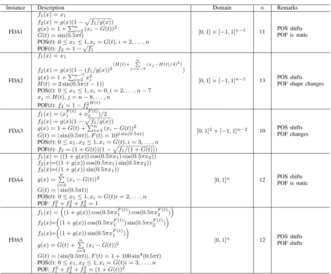
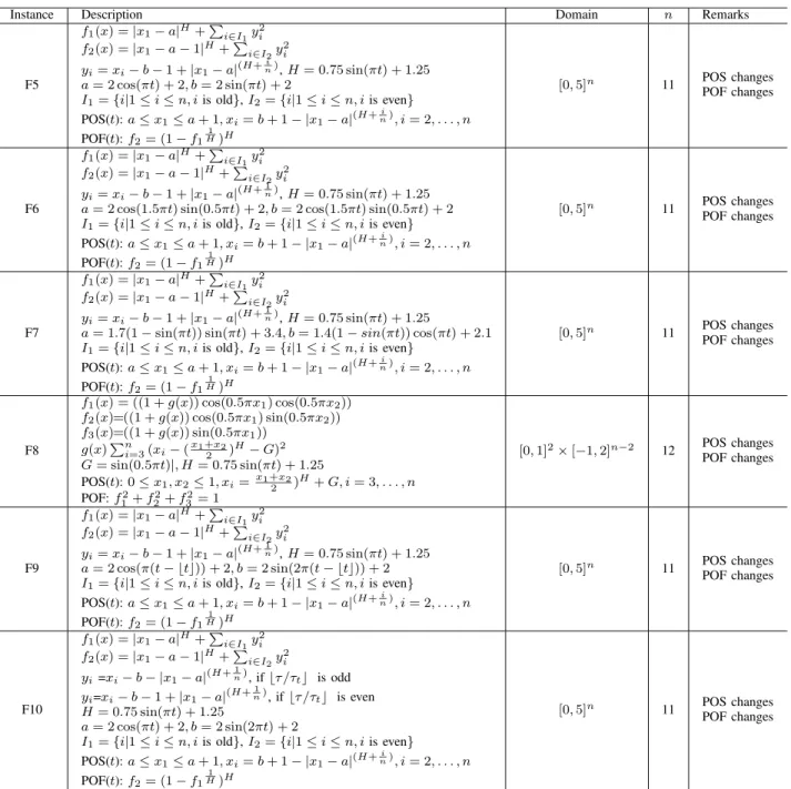
Twenty-one test problems, including five FDA [15] prob-lems, three dMOP [18] probprob-lems, six ZJZ problems (F5-F10) [54], and seven UDF [4] problems, are used to assess our proposed algorithm in comparison with other algorithms. The time instance t involved in these problems is defined as t = 1
nt⌊
τ
τt⌋ (where nt, τt, and τ represent the severity of
change, the frequency of change, and the iteration counter, respectively). The definition of these problems can be found in the supplementary material of this paper. Note that, some problems have been modified to implement our experiments, and most of the test problems have periodical changes.
B. Compared Algorithms
Four popular DMOEAs are used for comparison in our em-pirical studies. They are the MOEA based on decomposition (MOEA/D) [51], dynamic version of NSGA-II (DNSGA-II) [12], dCOEA [18], and PPS [54], representing different classes of metaheuristics. The following gives a brief description of each compared algorithm.
1) MOEA/D: as a representative of decomposition-based algorithms, MOEA/D [51] converts a mutiobjective problem by aggregation functions into a number of
single-objective subproblems and optimizes them simul-taneously. MOEA/D maintains population diversity by the diversity of subproblems, and a fast convergence can be achieved by defining a neighbourhood for each sub-problem and performing mating selection and solution update within this neighbourhood. Due to these features, MOEA/D has gained increasing popularity in recent years and has become a benchmark algorithm in static multiobjective optimization. In this paper, the modified version of the weighted Tchebycheff approach used in [49] is adopted as the aggregation function for MOEA/D because it has been recently proved to provide better distribution than its original version. Also, a limited number nr of solutions will be replaced by any new
solution, as suggested in [31].
2) DNSGA-II: it is a dynamic version of the popular NSGA-II algorithm [13], which is a representative of Pareto-dominance based MOEAs. To make it suitable for handling dynamic optimization problems, Deb et al. [12] adapted NSGA-II by replacing some population mem-bers with either randomly created solutions or mutated solutions of existing solutions if a change occurs. While the former may perform better in environments with se-vere changes, the latter may work well on DMOPs with moderate changes. In our experiment, the latter method is adopted as it shows slightly better performance than the former in the study of [12].
3) dCOEA: it hybridizes competitive and cooperative mechanisms observed in nature to solve static MOPs and to track the changing POF in a dynamic environment [18]. dCOEA uses a fixed number of archived solutions to detect changes, and if detected, its competitive mech-anism will be started to assess the potential of existing information of various subpopulations. To increase di-versity after a change, dCOEA also introduces stochastic solutions into the competitive pool. Besides, dCOEA uses an additional external population to store useful but outdated archived solutions, hoping to help the evolving population quickly adapt to the new environment by exploiting these history information. It has been shown that dCOEA is very promising for handling dynamic environments [18], [24].
4) PPS: it is a representative of prediction-based methods that model the movement track of the POF or POS in dynamic environments and then use this model to predict the new location of POS. In PPS [54], the POS information is divided into two parts: the population centre and manifold. Based on the archived population centres over a number of continuous time steps, PPS employs a univariate autoregression model to predict the next population centre. Likewise, previous manifolds are used to predict the next manifold. When a change occurs, the initial population for the new environment is created from the predicted centre and manifold. PPS has been proved to be very competitive for dynamic optimization when it is incorporated with an estimation of distribution algorithm [53], and it outperforms other predictive models [54].
C. Performance Metric
In our experimental studies, we adopt the following perfor-mance metrics, as they can help deeply investigate algorithms’ performance regarding convergence, distribution, and diversity.
1) Inverted Generational Distance (IGD): The IGD [49], [50], [54] measures both the convergence and diversity of found solutions by an algorithm. Let P OF be a set of uniformly distributed points in the true POF, andP OF∗
be an approximation of the POF. The IGD is calculated as follows:
IGD= 1 nP OF nP OF X i=1 di (8)
wherenP OF =|P OF|,di is the Euclidean distance between
theith member inP OF and its nearest member in P OF∗ .
2) Schott’s Spacing Metric (S): Schott [39] developed this kind of metric with regard to the distribution of the discovered Pareto front. S measures how evenly the members inP OF∗ are distributed, and is computed as:
S= v u u t 1 nP OF∗−1 nP OF∗ X i=1 (Di−D)2 (9)
whereDiis the Euclidean distance between theith member in
P OF∗
and its nearest member inP OF∗
andDis the average value ofDi.
3) Maximum Spread (MS): The MS [17] measures to what extent the obtainedP OF∗
coversP OF: M S= v u u t1 M M X k=1 " min[P OFk, P OFk∗]−max[P OFk, P OFk∗] P OFk−P OFk #2 (10)
whereP OFk andP OFk are the maximum and minimum of
thekth objective inP OF, respectively; Similarly,P OF∗ k and
P OF∗
k are the maximum and minimum of the kth objective
inP OF∗
, respectively.
4) Hypervolume Difference (HVD): The HVD [55] mea-sures the gap between the hypervolume of the obtainedP OF∗ and that of the trueP OF:
HV D=HV(P OF)−HV(P OF∗
) (11)
whereHV(S)is the hypervolume of a set S. The reference point for the computation of hypervolume is (z1+ 0.5, z2+ 0.5,· · ·, zM+0.5), wherezjis the maximum value of thej-th
objective of the true POF andM is the number of objectives.
D. Parameter Settings
The parameters of the MOEAs considered in the experi-ment were referenced from their original papers. Some key parameters in these algorithms were set as follows:
1) Population size: The population size (N) for all the test problems was set to 100. To make MOEA/D have 100 subproblems for three-objective FDA4 and FDA5, we first uniformly generate around 1000 weight vectors using the simplex-lattice design [51], then prune them to 100 using the farthest first method [10], [11]. 2) Parameter settings for SGEA: These parameters were
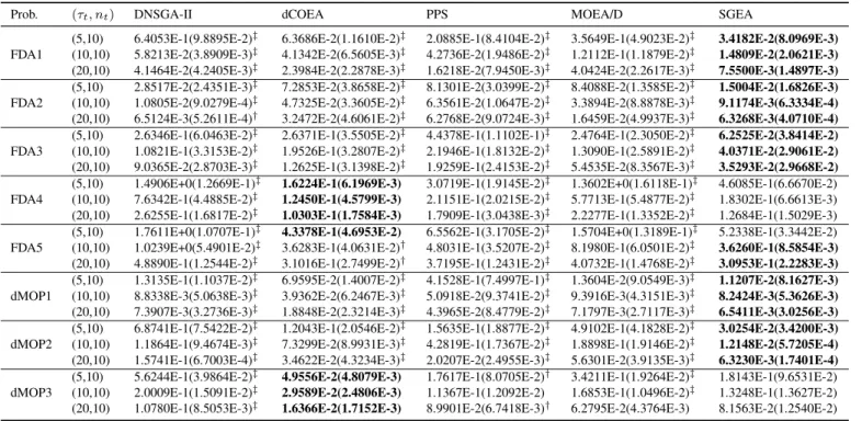
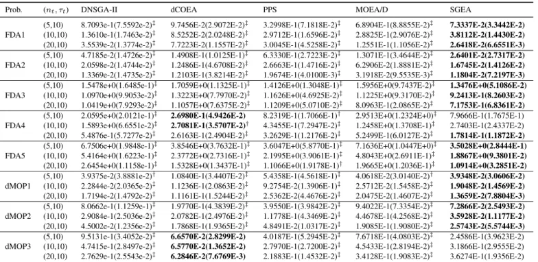
TABLE I
MEAN AND STANDARD DEVIATION VALUES OFSPMETRIC OBTAINED BY FIVE ALGORITHMS
Prob. (τt, nt) DNSGA-II dCOEA PPS MOEA/D SGEA
(5,10) 2.5421E-2(2.5497E-3)‡ 3.3966E-2(2.6330E-3)‡ 6.1386E-2(1.6514E-2)‡ 4.6542E-1(1.4472E-1)‡ 1.3267E-2(1.1095E-3) FDA1 (10,10) 1.0136E-2(7.4361E-3)‡ 1.8316E-2(1.4011E-3)‡ 1.7072E-2(6.5312E-3)‡ 4.8939E-1(1.9408E-1)‡ 7.5411E-3(5.8178E-4)
(20,10) 6.7495E-3(7.3732E-4)‡ 8.9615E-3(7.8094E-4)‡ 5.7913E-2(1.6129E-2)‡ 3.5391E-1(1.6524E-1)‡ 3.9986E-3(2.5969E-4) (5,10) 7.6448E-3(3.1834E-4) 2.7693E-2(3.9466E-3)‡ 2.4594E-2(6.0101E-3)‡ 1.8142E-2(2.8950E-2)‡ 9.4054E-3(1.6736E-3) FDA2 (10,10) 5.3715E-3(3.3796E-4) 1.5614E-2(2.8655E-3)‡ 1.7122E-2(3.9192E-3)‡ 1.5625E-2(2.4152E-2)‡ 6.5871E-3(8.7753E-4) (20,10) 5.0340E-3(1.3246E-4)† 8.0937E-3(2.0835E-3)‡ 1.8392E-2(4.0463E-3)‡ 1.0903E-2(4.8363E-3)‡ 4.9516E-3(4.9187E-4) (5,10) 1.7052E-2(2.3120E-3) 3.3698E-2(1.6310E-2)† 5.2045E-2(9.7887E-3)‡ 8.3517E-2(4.6837E-2)‡ 3.1669E-2(4.1347E-3) FDA3 (10,10) 1.1167E-2(1.9011E-3) 1.7698E-2(9.1874E-3) 1.6536E-2(4.1971E-3) 4.6011E-2(1.8288E-2)‡ 2.4160E-2(1.8298E-3) (20,10) 8.2268E-3(1.7859E-3) 1.2049E-2(6.1286E-3) 9.0478E-3(2.0861E-3) 2.9416E-2(8.6135E-3)‡ 2.2741E-2(9.9650E-4) (5,10) 1.2706E-1(5.5003E-3)‡ 5.9217E-2(4.6346E-3) 1.0232E-1(9.7961E-3)† 1.8035E-1(3.2800E-2)‡ 8.7427E-2(7.6848E-3) FDA4 (10,10) 9.1659E-2(3.8467E-3)‡ 3.8658E-2(3.2771E-3) 6.0989E-2(1.0643E-2)‡ 1.6494E-1(2.9433E-2)‡ 4.1252E-2(2.9737E-3) (20,10) 5.5146E-2(2.1395E-3)‡ 2.7830E-2(1.5839E-3)† 4.8519E-2(2.9057E-3)‡ 1.6572E-1(2.5986E-2)‡ 2.5354E-2(2.8502E-3) (5,10) 1.5306E-1(5.0947E-3)‡ 9.9019E-2(8.8149E-3)‡ 1.4717E-1(1.1045E-2)‡ 1.5505E-1(1.4762E-2)‡ 8.2228E-2(4.2364E-3) FDA5 (10,10) 1.1245E-1(3.9588E-3)‡ 6.3211E-2(4.8740E-3)‡ 1.0820E-1(8.7265E-3)‡ 1.2839E-1(1.5067E-2)‡ 4.5009E-2(2.6441E-3)
(20,10) 8.0300E-2(2.3006E-3)‡ 4.9950E-2(3.1582E-3)‡ 8.6349E-2(4.1808E-3)‡ 1.0497E-1(7.8394E-3)‡ 3.0379E-2(6.7640E-4) (5,10) 5.3389E-3(7.8416E-4)‡ 8.4983E-2(5.2562E-3)‡ 1.0375E-1(7.8713E-2)‡ 4.1207E-2(1.1779E-1)‡ 3.4712E-3(5.4488E-4)
dMOP1 (10,10) 5.5311E-3(1.3101E-3)‡ 1.5696E-2(9.5712E-3)‡ 2.5068E-2(2.4719E-2)‡ 5.6413E-2(2.0924E-1)‡ 2.7029E-3(3.0835E-4)
(20,10) 5.2961E-3(2.7514E-4)‡ 6.3031E-3(6.6072E-4)‡ 1.4722E-2(2.0239E-2)‡ 2.6844E-2(8.1479E-2)‡ 2.5010E-3(2.5768E-4) (5,10) 1.6538E-2(1.7941E-3)‡ 6.0455E-2(2.1579E-3)‡ 2.7767E-2(4.5722E-3)‡ 1.4701E-1(5.3676E-2)‡ 1.3177E-2(1.4569E-3) dMOP2 (10,10) 1.0690E-2(5.3335E-4)‡ 3.0587E-2(3.9867E-3)‡ 1.1608E-2(2.7373E-3)‡ 1.4459E-1(5.3516E-2)‡ 6.6710E-3(5.8584E-4)
(20,10) 6.2086E-3(1.9806E-4)‡ 1.4253E-2(1.7038E-3)‡ 6.2807E-3(1.1104E-3)‡ 1.4322E-1(6.6231E-2)‡ 3.9175E-3(2.9561E-4) (5,10) 1.4393E-2(1.2499E-3)‡ 3.3786E-2(5.5519E-3)‡ 2.7518E-2(4.8871E-3)‡ 2.7281E-2(2.2967E-2)‡ 9.5664E-3(9.9353E-4)
dMOP3 (10,10) 8.1655E-3(6.5231E-4)‡ 1.5418E-2(1.0978E-3)‡ 1.6453E-2(2.3904E-3)‡ 1.2555E-2(2.0652E-3)‡ 5.4336E-3(6.0751E-4)
(20,10) 5.3930E-3(5.5912E-4)‡ 7.3129E-3(3.9782E-4)‡ 1.1264E-2(1.7604E-3)‡ 9.9081E-3(1.4603E-3)‡ 4.2793E-3(5.3812E-4)
‡and†indicate SGEA performs significantly better than and equivalently to the corresponding algorithm, respectively.
Specifically, the crossover probability was pc = 1.0
and its distribution index was ηc = 20. The mutation
probability waspm= 1/nand its distributionηm= 20.
The archive size was the same as the population size. 3) Stopping criterion and the number of executions: Each
algorithm terminates after a pre-specified number of generations and should cover all possible changes. To minimize the effect of static optimization, we gave 50 generations for each algorithm before the first change occurs. The total number of generations was set to
3ntτt+ 50, which ensures there are3ntchanges during
the evolution. Additionally, each algorithm was executed 30 independent times on each test instance.
4) The neighbourhood size and the numbernrof solutions
allowed to replace in MOEA/D were set to 20 and 2, respectively.
5) For all the algorithms, the maximum 10% population members were chosen for change detection. For the steady-state MOEA/D, it used the same change detection mechanism as SGEA, and population re-evaluation for change response.
6) The number of uniformly sampled points on the true POF was set to 500 and 990 for the computation of IGD for bi- and three-objective problems, respectively.
IV. EXPERIMENTALRESULTS ANDANALYSIS
A. Results on FDA and dMOP Problems
To study the impact of change frequency on algorithms’ ability in dynamic environments, the severity of change (nt)
was fixed to 10, and the frequency of change (τt) was set
to 5, 10, and 20, respectively. The obtained average SP, MS, IGD, and HVD results over a series of time windows and their
standard deviation values are presented in Tables I, II, III, and IV, respectively, where the best values obtained by one of five algorithms are highlighted in bold face. The Wilcoxon rank-sum test [46] is carried out to indicate significance between different results at the 0.05 significance level.
It can be observed from Table I that SGEA obtains the best results on the majority of the tested FDA and dMOP instances, implying that it maintains better distribution of its approximations over changes than the other compared algorithms in most cases. However, it performs slightly worse than DNSGA-II for FDA2 and FDA3, and dCOEA for FDA4 with fast changes (i.e., τt = 5 and 10). For all the tested
instances, both PPS and MOEA/D fail to show encouraging performance on the SP metric, and MOEA/D seems struggling for maintaining a uniform distribution of its obtained POF for dynamic optimization, as indicated by the large SP values in Table I.
As shown in Table II, the results on the MS metric are quite divergent. DNSGA-II and SGEA obtain a spread coverage for FDA2, FDA4, and FDA5, although DNSGA-II provides slightly better MS values than SGEA. For problems FDA1, FDA3, and dMOP2, SGEA significantly outperforms the other algorithms by a clear margin in terms of the MS metric. PPS and MOEA/D cover the POF very well for two three-objective problems, i.e., FDA4 and FDA5, and all the algo-rithms perform similarly on dMOP1 except dCOEA, whose MS values are not very competitive in this case. To have a better understanding of how algorithms’ MS performance can be affected by different dynamisms, we discuss a little bit more on FDA3 and dMOP3. FDA3 is a problem in which environmental changes shift the POS and affect the density of points on the POF whereas dMOP3 is a problem where
TABLE II
MEAN AND STANDARD DEVIATION VALUES OFMSMETRIC OBTAINED BY FIVE ALGORITHMS
Prob. (τt, nt) DNSGA-II dCOEA PPS MOEA/D SGEA
(5,10) 6.8875E-1(6.9604E-2)‡ 8.6361E-1(2.5899E-2)‡ 8.7571E-1(3.3122E-2)‡ 8.2378E-1(2.2483E-2)‡ 9.3411E-1(3.2794E-2) FDA1 (10,10) 9.2689E-1(1.9129E-2)‡ 8.9378E-1(2.2115E-2)‡ 9.6555E-1(1.2319E-2)‡ 9.2142E-1(1.6053E-2)‡ 9.7277E-1(1.0854E-2)
(20,10) 9.8453E-1(2.1657E-3)† 9.2981E-1(1.2003E-2)‡ 9.8426E-1(4.8155E-3)† 9.6140E-1(8.4959E-3)‡ 9.8810E-1(6.2816E-3) (5,10) 9.9649E-1(4.2818E-3)† 8.1389E-1(4.8855E-2)‡ 9.0733E-1(5.3057E-2)‡ 9.4951E-1(3.7796E-2)‡ 9.9231E-1(5.2065E-3) FDA2 (10,10) 9.9730E-1(2.6637E-3)† 8.7511E-1(2.9208E-2)‡ 9.3410E-1(1.2746E-2)‡ 9.6362E-1(2.5629E-2)‡ 9.9308E-1(3.3464E-3) (20,10) 9.9786E-1(1.9825E-3) 9.1688E-1(3.2152E-2)‡ 9.3897E-1(7.2423E-3)‡ 9.7535E-1(1.8048E-2)‡ 9.9342E-1(2.6409E-3) (5,10) 6.3387E-1(1.1045E-1)‡ 5.0510E-1(4.5498E-2)‡ 6.0036E-1(3.4102E-2)‡ 7.3593E-1(9.3637E-2)‡ 8.8834E-1(8.9085E-2) FDA3 (10,10) 7.6418E-1(7.9082E-2)‡ 5.7869E-1(3.6421E-2)‡ 6.0893E-1(2.6990E-2)‡ 8.2943E-1(8.4314E-2)‡ 9.3342E-1(7.1125E-2)
(20,10) 7.8775E-1(7.2659E-2)‡ 6.8023E-1(4.3336E-2)‡ 6.0760E-1(2.4411E-2)‡ 8.8984E-1(2.1886E-2)‡ 9.4731E-1(7.2987E-2) (5,10) 9.9999E-1(3.2759E-6)† 9.6390E-1(7.4777E-3)‡ 9.9823E-1(7.5711E-4)‡ 9.9999E-1(2.1721E-6)† 9.9997E-1(1.9039E-5) FDA4 (10,10) 1.0000E+0(7.8284E-7) 9.7421E-1(6.0289E-3)‡ 9.9903E-1(1.2185E-4)‡ 9.9999E-1(8.5330E-7) 9.9995E-1(2.6230E-5) (20,10) 1.0000E+0(3.0455E-7) 9.8552E-1(2.3528E-3)‡ 9.9904E-1(9.8111E-5)‡ 1.0000E+0(2.6739E-7) 9.9992E-1(2.5034E-5) (5,10) 9.9999E-1(2.0403E-6) 9.3043E-1(3.7021E-2)‡ 9.9758E-1(2.6961E-3) 9.9866E-1(3.2365E-3) 9.9442E-1(8.0786E-3) FDA5 (10,10) 1.0000E+0(4.3629E-7) 9.5871E-1(3.5891E-2)‡ 9.9781E-1(3.8432E-3)‡ 9.9995E-1(1.4197E-4) 9.9949E-1(7.9814E-4) (20,10) 1.0000E+0(7.6916E-8) 9.7908E-1(1.9611E-2)‡ 9.9955E-1(1.7863E-4)† 9.9999E-1(7.9466E-7) 9.9993E-1(5.9215E-5) (5,10) 9.5971E-1(4.5522E-2)† 8.2629E-1(4.1500E-2)‡ 9.3007E-1(6.7780E-2)‡ 9.6544E-1(3.8454E-2)† 9.5950E-1(3.3426E-2) dMOP1 (10,10) 9.8083E-1(2.0385E-2)† 8.8318E-1(2.5097E-2)‡ 9.7105E-1(3.3827E-2)‡ 9.8276E-1(1.5980E-2)† 9.8351E-1(1.3118E-2)
(20,10) 9.8836E-1(1.1924E-2)† 9.3962E-1(1.0940E-2)‡ 9.8192E-1(1.8910E-2)† 9.8869E-1(1.0211E-2)‡ 9.8534E-1(1.2710E-2) (5,10) 7.1985E-1(9.8981E-2)‡ 7.4615E-1(5.4804E-2)‡ 8.5360E-1(1.3935E-2)‡ 7.9673E-1(1.2783E-2)‡ 9.4952E-1(1.3091E-2) dMOP2 (10,10) 8.8398E-1(1.0456E-2)‡ 8.1368E-1(2.5334E-2)‡ 9.5016E-1(1.6218E-2)‡ 8.8264E-1(1.4109E-2)‡ 9.8099E-1(4.5689E-3)
(20,10) 9.8039E-1(3.2935E-2)‡ 9.0203E-1(1.6144E-2)‡ 9.7464E-1(2.6993E-3)‡ 9.5552E-1(5.9188E-3)‡ 9.9251E-1(1.4628E-3) (5,10) 4.3016E-1(2.2614E-2)‡ 8.7837E-1(2.1444E-2) 8.5479E-1(1.3831E-2) 5.0950E-1(3.1263E-2)† 4.9760E-1(2.2063E-2) dMOP3 (10,10) 5.3193E-1(2.1894E-2)† 9.1097E-1(1.1716E-2) 8.8793E-1(9.6772E-3) 6.3606E-1(1.8266E-2) 5.7573E-1(2.9590E-2) (20,10) 6.2492E-1(1.9883E-2)‡ 9.4844E-1(1.1052E-2) 9.0666E-1(9.4326E-3) 7.7993E-1(1.9421E-2) 6.8486E-1(2.9571E-2) ‡and†indicate SGEA performs significantly better than and equivalently to the corresponding algorithm, respectively.
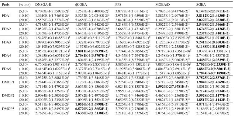
TABLE III
MEAN AND STANDARD DEVIATION VALUES OFIGDMETRIC OBTAINED BY FIVE ALGORITHMS
Prob. (τt, nt) DNSGA-II dCOEA PPS MOEA/D SGEA
(5,10) 6.4053E-1(9.8895E-2)‡ 6.3686E-2(1.1610E-2)‡ 2.0885E-1(8.4104E-2)‡ 3.5649E-1(4.9023E-2)‡ 3.4182E-2(8.0969E-3)
FDA1 (10,10) 5.8213E-2(3.8909E-3)‡ 4.1342E-2(6.5605E-3)‡ 4.2736E-2(1.9486E-2)‡ 1.2112E-1(1.1879E-2)‡ 1.4809E-2(2.0621E-3)
(20,10) 4.1464E-2(4.2405E-3)‡ 2.3984E-2(2.2878E-3)‡ 1.6218E-2(7.9450E-3)‡ 4.0424E-2(2.2617E-3)‡ 7.5500E-3(1.4897E-3)
(5,10) 2.8517E-2(2.4351E-3)‡ 7.2853E-2(3.8658E-2)‡ 8.1301E-2(3.0399E-2)‡ 8.4088E-2(1.3585E-2)‡ 1.5004E-2(1.6826E-3)
FDA2 (10,10) 1.0805E-2(9.0279E-4)‡ 4.7325E-2(3.3605E-2)‡ 6.3561E-2(1.0647E-2)‡ 3.3894E-2(8.8878E-3)‡ 9.1174E-3(6.3334E-4)
(20,10) 6.5124E-3(5.2611E-4)† 3.2472E-2(4.6061E-2)‡ 6.2768E-2(9.0724E-3)‡ 1.6459E-2(4.9937E-3)‡ 6.3268E-3(4.0710E-4)
(5,10) 2.6346E-1(6.0463E-2)‡ 2.6371E-1(3.5505E-2)‡ 4.4378E-1(1.1102E-1)‡ 2.4764E-1(2.3050E-2)‡ 6.2525E-2(3.8414E-2)
FDA3 (10,10) 1.0821E-1(3.3153E-2)‡ 1.9526E-1(3.2807E-2)‡ 2.1946E-1(1.8132E-2)‡ 1.3090E-1(2.5891E-2)‡ 4.0371E-2(2.9061E-2)
(20,10) 9.0365E-2(2.8703E-3)‡ 1.2625E-1(3.1398E-2)‡ 1.9259E-1(2.4153E-2)‡ 5.4535E-2(8.3567E-3)‡ 3.5293E-2(2.9668E-2)
(5,10) 1.4906E+0(1.2669E-1)‡ 1.6224E-1(6.1969E-3) 3.0719E-1(1.9145E-2)‡ 1.3602E+0(1.6118E-1)‡ 4.6085E-1(6.6670E-2) FDA4 (10,10) 7.6342E-1(4.4885E-2)‡ 1.2450E-1(4.5799E-3) 2.1151E-1(2.0215E-2)‡ 5.7713E-1(5.4877E-2)‡ 1.8302E-1(6.6613E-3) (20,10) 2.6255E-1(1.6817E-2)‡ 1.0303E-1(1.7584E-3) 1.7909E-1(3.0438E-3)‡ 2.2277E-1(1.3352E-2)‡ 1.2684E-1(1.5029E-3) (5,10) 1.7611E+0(1.0707E-1)‡ 4.3378E-1(4.6953E-2) 6.5562E-1(3.1705E-2)‡ 1.5704E+0(1.3189E-1)‡ 5.2338E-1(3.3442E-2) FDA5 (10,10) 1.0239E+0(5.4901E-2)‡ 3.6283E-1(4.0631E-2)† 4.8031E-1(3.5207E-2)‡ 8.1980E-1(6.0501E-2)‡ 3.6260E-1(8.5854E-3) (20,10) 4.8890E-1(1.2544E-2)‡ 3.1016E-1(2.7499E-2)† 3.7195E-1(1.2431E-2)‡ 4.0732E-1(1.4768E-2)‡ 3.0953E-1(2.2283E-3)
(5,10) 1.3135E-1(1.1037E-2)‡ 6.9595E-2(1.4007E-2)‡ 4.1528E-1(7.4997E-1)‡ 1.3604E-2(9.0549E-3)‡ 1.1207E-2(8.1627E-3)
dMOP1 (10,10) 8.8338E-3(5.0638E-3)‡ 3.9362E-2(6.2467E-3)‡ 5.0918E-2(9.3741E-2)‡ 9.3916E-3(4.3151E-3)‡ 8.2424E-3(5.3626E-3) (20,10) 7.3907E-3(3.2736E-3)‡ 1.8848E-2(2.3214E-3)‡ 4.3965E-2(8.4779E-2)‡ 7.1797E-3(2.7117E-3)‡ 6.5411E-3(3.0256E-3)
(5,10) 6.8741E-1(7.5422E-2)‡ 1.2043E-1(2.0546E-2)‡ 1.5635E-1(1.8877E-2)‡ 4.9102E-1(4.1828E-2)‡ 3.0254E-2(3.4200E-3)
dMOP2 (10,10) 1.1864E-1(9.4674E-3)‡ 7.3299E-2(8.9931E-3)‡ 4.2819E-1(1.7367E-2)‡ 1.8898E-1(1.9146E-2)‡ 1.2148E-2(5.7205E-4) (20,10) 1.5741E-1(6.7003E-4)‡ 3.4622E-2(4.3234E-3)‡ 2.0207E-2(2.4955E-3)‡ 5.6301E-2(3.9135E-3)‡ 6.3230E-3(1.7401E-4)
(5,10) 5.6244E-1(3.9864E-2)‡ 4.9556E-2(4.8079E-3) 1.7617E-1(8.0705E-2)† 3.4211E-1(1.9264E-2)‡ 1.8143E-1(9.6531E-2) dMOP3 (10,10) 2.0009E-1(1.5091E-2)‡ 2.9589E-2(2.4806E-3) 1.1367E-1(1.2092E-2) 1.6853E-1(1.0496E-2)‡ 1.3248E-1(1.3627E-2) (20,10) 1.0780E-1(8.5053E-3)‡ 1.6366E-2(1.7152E-3) 8.9901E-2(6.7418E-3)† 6.2795E-2(4.3764E-3) 8.1563E-2(1.2540E-2) ‡and†indicate SGEA performs significantly better than and equivalently to the corresponding algorithm, respectively.
the population diversity can decrease dramatically. The results of MS show that, for FDA3, SGEA can maintain a good coverage of the POF when the other algorithms perform poorly. However, this is not the case for dMOP3, where only dCOEA and PPS are able to distribute their obtained solutions widely on the POF. This means that the change response mechanisms in DNSGA-II, MOEA/D, and SGEA may face big
challenges when dynamisms drastically aggravate population diversity.
Since the IGD metric mainly depends on the closeness, distribution, and coverage of an approximation to the true POF, we can use IGD together with SP and MS to deeply and extensively reveal the algorithms’ performance on the test instances. Table III clearly shows that, SGEA performs the
TABLE IV
MEAN AND STANDARD DEVIATION VALUES OFHVDMETRIC OBTAINED BY FIVE ALGORITHMS
Prob. (τt, nt) DNSGA-II dCOEA PPS MOEA/D SGEA
(5,10) 8.7093E-1(7.5592E-2)‡ 1.2585E-1(2.4080E-2)‡ 3.8772E-1(1.0116E-1)‡ 7.7026E-1(9.4376E-2)‡ 8.1493E-2(2.0911E-2) FDA1 (10,10) 1.3610E-1(1.7463E-2)‡ 8.5252E-2(2.0248E-2)‡ 2.9712E-1(1.6596E-2)‡ 2.8825E-1(2.9076E-2)‡ 3.8112E-2(1.4430E-2)
(20,10) 3.5539E-2(1.3774E-2)‡ 5.4656E-2(1.6343E-2)‡ 2.8401E-1(1.5220E-2)‡ 1.3478E-1(9.2613E-3)‡ 2.0270E-2(1.2830E-2) (5,10) 4.7185E-2(1.4726E-2)‡ 1.8564E-1(6.4420E-2)‡ 3.2184E-1(6.7336E-2)‡ 1.3022E-1(2.5946E-2)‡ 2.5498E-2(1.3466E-2) FDA2 (10,10) 2.0598E-2(1.4744E-2)‡ 1.2486E-1(4.6708E-2)‡ 2.6663E-1(1.4716E-2)‡ 6.2906E-2(1.8881E-2)‡ 1.6745E-2(1.4126E-2)
(20,10) 1.3369E-2(1.4735E-2)‡ 8.6455E-2(7.0196E-2)‡ 2.5527E-1(9.4754E-3)‡ 3.2497E-2(1.4799E-2)‡ 1.2377E-2(1.4101E-2) (5,10) 1.5478E+0(1.6485E-1)‡ 1.4594E+0(8.5119E-2)‡ 1.7549E+0(1.8461E-1)‡ 1.6606E+0(7.8359E-2)‡ 9.8045E-1(1.0710E-1) FDA3 (10,10) 1.0970E+0(9.9053E-2)‡ 1.3223E+0(7.7970E-2)‡ 1.1626E+0(4.6925E-2)‡ 1.1225E+0(9.3170E-2)‡ 9.2413E-1(8.2603E-2)
(20,10) 1.0419E+0(7.9293E-2)‡ 1.1578E+0(6.6326E-2)‡ 1.0365E+0(7.4288E-2)‡ 9.4755E-1(2.2550E-2)‡ 9.1188E-1(8.1889E-2) (5,10) 2.0595E+0(2.0121E-1)‡ 3.8011E-1(2.6939E-2) 7.7744E-1(6.8856E-2)‡ 3.9719E+0(1.6351E+0)‡ 1.0379E+0(1.3381E-1) FDA4 (10,10) 1.5893E+0(6.6551E-2)‡ 2.7081E-1(3.5707E-2)† 4.3455E-1(7.2947E-2)‡ 1.2458E+0(1.3708E-1)‡ 2.7403E-1(2.4337E-2)
(20,10) 5.4876E-1(5.7277E-2)‡ 1.8048E-1(2.4395E-2)‡ 3.3435E-1(8.3758E-3)‡ 4.3462E-1(5.0662E-2)‡ 1.4480E-1(2.0339E-2) (5,10) 6.7506E+0(1.9848E-1)‡ 2.7667E+0(2.8579E-1)‡ 3.8869E+0(3.1382E-1)‡ 7.0876E+0(1.0641E+0)‡ 2.7020E+0(2.2339E-1) FDA5 (10,10) 5.4164E+0(1.6223E-1)‡ 2.3772E+0(2.7316E-1)‡ 2.1995E+0(3.9061E-1)‡ 4.8043E+0(2.6911E-1)‡ 1.8867E+0(9.3801E-2)
(20,10) 2.6454E+0(1.1158E-1)‡ 2.0207E+0(1.8696E-1)‡ 1.0481E+0(1.1778E-1) 2.1517E+0(1.0853E-1)‡ 1.7874E+0(7.1890E-2) (5,10) 3.9375E-2(3.8881E-2)† 1.7307E-1(3.3448E-2)‡ 2.8629E-1(3.6238E-1)‡ 4.6453E-2(3.6865E-2)‡ 3.7523E-2(2.5376E-2)
DMOP1 (10,10) 2.2844E-2(2.0365E-2)‡ 1.1236E-1(2.0863E-2)‡ 9.2754E-2(1.3906E-1)‡ 2.5712E-2(1.5458E-2)‡ 1.9048E-2(1.4569E-2)
(20,10) 1.7194E-2(1.4792E-2)† 5.6555E-2(8.1366E-3)‡ 6.0241E-2(8.1387E-2)‡ 1.5920E-2(7.9781E-3) 1.8012E-2(1.3010E-2) (5,10) 8.0662E-1(1.1259E-1)‡ 3.0338E-1(4.9212E-2)‡ 3.9550E-1(3.9842E-2)‡ 9.0438E-1(7.3270E-2)‡ 8.7174E-2(1.9234E-2) DMOP2 (10,10) 2.9084E-1(2.5036E-2)‡ 2.0782E-1(2.4976E-2)‡ 1.1778E-1(4.3469E-2)‡ 4.4678E-1(4.2568E-2)‡ 3.5928E-2(1.1177E-2)
(20,10) 4.5002E-2(1.2356E-2)‡ 1.0906E-1(1.5524E-2)‡ 5.6596E-2(6.2322E-3)‡ 1.9824E-1(1.4847E-2)‡ 1.8517E-2(1.1142E-2) (5,10) 9.5131E-1(3.4052E-2)‡ 1.0526E-1(1.6998E-2) 4.2264E-1(1.5786E-2)† 7.6163E-1(5.3913E-2)† 4.0715E-1(2.4743E-2) DMOP3 (10,10) 4.7415E-1(2.8497E-2)‡ 6.5770E-2(1.3652E-2) 2.7970E-1(2.7200E-2) 4.5433E-1(2.8194E-2)‡ 3.1866E-1(2.9555E-2) (20,10) 2.7629E-1(2.5543E-2)‡ 3.6360E-2(1.3138E-2) 2.2118E-1(1.5326E-2)† 2.8764E-1(2.0740E-2)‡ 2.1541E-1(3.0679E-2) ‡and†indicate SGEA performs significantly better than and equivalently to the corresponding algorithm, respectively.
best on the majority of the test instances and mainly loses on FDA4 and dMOP3, where dCOEA is the best performer, in terms of the IGD metric. Clearly, the uncompetitive dis-tribution (i.e., slightly large SP metric) and poor coverage (i.e., relatively small MS metric) of obtained approximations are the main reasons for the low performance of SGEA on FDA4 and dMOP3, respectively. However, good SP and MS values do not necessarily result in satisfying IGD metric, and this can be particularly observed from the case of DNSGA-II on FDA2, suggesting that DNSGA-II converges worse than SGEA although it provides the best SP and MS metrics on this problem. For PPS and MOEA/D, the IGD performance is not competitive in spite of their good spread performance for most of the test instances, and this may be caused by their poor solution distribution, as indicated by their large SP values.
Table IV presents the HVD metric obtained by five algo-rithms on the FDA and dMOP problems. The obtained HVD values are roughly consistent with the IGD ones illustrated in Table III. Clearly, SGEA is more promising than the other algorithms to solve most FDA and dMOP instances, but it is outperformed by dCOEA on FDA4 and DMOP3. Besides, the steady-state MOEA/D also shows some appealing results on FDA3 and DMOP1 whenτtequals 20, implying its
steady-state update method may be helpful for handling slow-changing environments.
It can also be observed from the results of the three used metrics that, the frequency of change has a significant effect on algorithms’ performance, and the effect decreases when environmental changes become slow. For two three-objective problems, i.e., FDA4 and FDA5, DNSGA-II and MOEA/D are most influenced by frequent changes and struggle to push their populations toward the POF, as indicated by their large IGD
and HVD values in Tables III and IV, respectively. Overall, dCOEA and SGEA seems less sensitive to the frequency of change, as can be seen from their gradual improvement on three metrics when τt increases from 5 to 20. On the
other hand, with the variation of frequency, there are drastic improvements on DNSGA-II, PPS, and MOEA/D in most of the test instances.
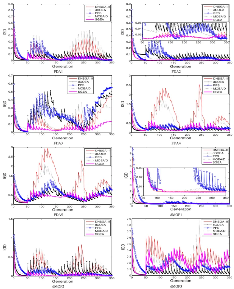
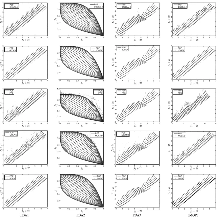
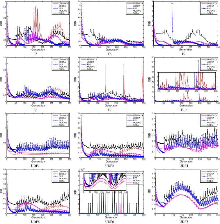
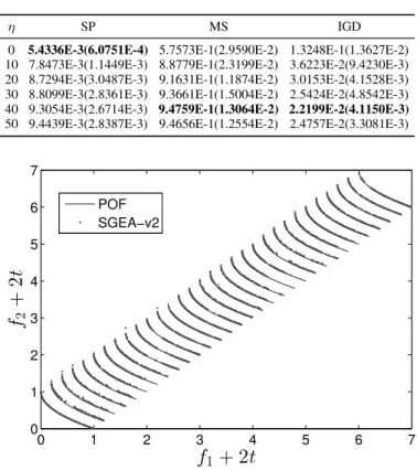
Apart from tabular presentation, we provide evolution curves of the average IGD values on the test instances in Fig. 1. It can be clearly seen that, compared with the other algorithms, SGEA responds to changes more stably and recovers faster for most of the test problems, thereby obtaining higher con-vergence performance. The only exception is dMOP3, where dCOEA performs the best, and due to the lack of population diversity (indicated by poor MS values) when a change oc-curs, the IGD values obtained by SGEA fluctuate widely on this problem. Despite that, SGEA performs similarly to PPS and better than DNSGA-II and MOEA/D on dMOP3. For a graphical view of algorithms’ tracking ability, we also plot their obtained POFs of FDA1, FDA2, FDA3 and dMOP3 over 31 time windows, which are shown in Fig. 2. Fig. 2 evidently shows that SGEA is very capable of tracking environmental changes, but may be of limited coverage if there is a significant diversity loss (e.g., on dMOP3) in dynamic environments.
B. Results on ZJZ and UDF Problems
Unlike the FDA and dMOP test suites, the ZJZ (F5-F10) [54] and UDF [4] test problems have nonlinear linkages between decision variables. Also, the ZJZ and UDF test suites introduces a number of new dynamic features which are not included in FDA and dMOP. Table V reports the HVD values obtained by five algorithms for these challenging problems
0 50 100 150 200 250 300 350 0 0.1 0.2 0.3 0.4 0.5 0.6 0.7 0.8 0.9 Generation IGD DNSGA−II dCOEA PPS MOEA/D SGEA 0 50 100 150 200 250 300 350 0 0.1 0.2 0.3 0.4 0.5 0.6 0.7 0.8 0.9 Generation IGD DNSGA−II dCOEA PPS MOEA/D SGEA 50 100 150 200 250 300 350 0 0.02 0.04 0.06 FDA1 FDA2 0 50 100 150 200 250 300 350 0 0.1 0.2 0.3 0.4 0.5 0.6 0.7 Generation IGD DNSGA−II dCOEA PPS MOEA/D SGEA 0 50 100 150 200 250 300 350 0 0.5 1 1.5 2 2.5 3 Generation IGD DNSGA−II dCOEA PPS MOEA/D SGEA FDA3 FDA4 0 50 100 150 200 250 300 350 0 0.5 1 1.5 2 2.5 3 Generation IGD DNSGA−II dCOEA PPS MOEA/D SGEA 0 50 100 150 200 250 300 350 0 1 2 3 4 5 6 7 8 9 Generation IGD DNSGA−II dCOEA PPS MOEA/D SGEA 50 100 150 200 250 300 350 0 0.01 0.02 0.03 FDA5 dMOP1 0 50 100 150 200 250 300 350 0 0.5 1 1.5 Generation IGD DNSGA−II dCOEA PPS MOEA/D SGEA 0 50 100 150 200 250 300 350 0 0.1 0.2 0.3 0.4 0.5 0.6 0.7 0.8 0.9 Generation IGD DNSGA−II dCOEA PPS MOEA/D SGEA dMOP2 dMOP3
Fig. 1. Evolution curves of averageIGDvalues for eight problems withτt= 10andnt= 10.
with (τt, nt) = (10,10), and the obtained SP, MS, and IGD
metric values can be found in the supplementary material. Compared with the average HVD values on FDA and dMOP problems given in Section IV-A, the average HVD
values obtained on ZJZ and UDF problems are generally much higher, implying that the optimization difficulties are increased in the ZJZ and UDF problems. Table V clearly shows that SGEA and PPS are top performers on these
0 1 2 3 4 5 6 7 0 1 2 3 4 5 6 7 f1+ 2t f1 + 2 t POF DNSGA−II 0 0.2 0.4 0.6 0.8 1 0 0.2 0.4 0.6 0.8 1 f1 f2 POF DNSGA−II 0 1 2 3 4 5 6 7 0 1 2 3 4 5 6 7 8 f1+ 2t f1 + 2 t POF DNSGA−II 0 1 2 3 4 5 6 7 0 1 2 3 4 5 6 7 f1+ 2t f2 + 2 t POF DNSGA−II 0 1 2 3 4 5 6 7 0 1 2 3 4 5 6 7 f1+ 2t f2 + 2 t POF dCOEA 0 0.2 0.4 0.6 0.8 1 0 0.2 0.4 0.6 0.8 1 f1 f2 POF dCOEA 0 1 2 3 4 5 6 7 0 1 2 3 4 5 6 7 8 f1+ 2t f1 + 2 t POF dCOEA 0 1 2 3 4 5 6 7 0 1 2 3 4 5 6 7 f1+ 2t f2 + 2 t POF dCOEA 0 1 2 3 4 5 6 7 0 1 2 3 4 5 6 7 f1+ 2t f2 + 2 t POF PPS 0 0.2 0.4 0.6 0.8 1 0 0.2 0.4 0.6 0.8 1 1.2 f1 f2 POF PPS 0 1 2 3 4 5 6 7 0 1 2 3 4 5 6 7 8 f1+ 2t f2 + 2 t POF PPS 0 2 4 6 8 0 1 2 3 4 5 6 7 8 f1+ 2t f2 + 2 t POF PPS 0 1 2 3 4 5 6 7 0 1 2 3 4 5 6 7 f1+ 2t f2 + 2 t POF MOEA/D 0 0.2 0.4 0.6 0.8 1 0 0.2 0.4 0.6 0.8 1 f1 f2 POF MOEA/D 0 1 2 3 4 5 6 7 0 1 2 3 4 5 6 7 8 f1+ 2t f2 + 2 t POF MOEA/D 0 1 2 3 4 5 6 7 0 1 2 3 4 5 6 7 f1+ 2t f2 + 2 t POF MOEA/D 0 1 2 3 4 5 6 7 0 1 2 3 4 5 6 7 f1+ 2t f2 + 2 t POF SGEA 0 0.2 0.4 0.6 0.8 1 0 0.2 0.4 0.6 0.8 1 f1 f2 POF SGEA 0 1 2 3 4 5 6 7 0 1 2 3 4 5 6 7 8 f1+ 2t f1 + 2 t POF SGEA 0 1 2 3 4 5 6 7 0 1 2 3 4 5 6 7 f1+ 2t f2 + 2 t POF SGEA
FDA1 FDA2 FDA3 dMOP3
Fig. 2. Obtained POFs for four problems withτt= 10andnt= 10.
difficult problems. SGEA obtains the best HVD values on some problems while PPS wins on others. SGEA performs significantly better than DNSGA-II on problems F5-F10, but this superiority disappears when they are compared on the UDF problems, and there is no much difference between them. This means SGEA has no much advantage in dealing with difficult variable-linkage UDF problems. PPS, which is not impressive for solving FDA and dMOP problems, shows very promising performance on some ZJZ and UDF problems. This is because PPS employs an estimation of distribution algorithm [53] as its reproduction operator. This operator can exploit problem specific knowledge, and hence is very helpful for solving variable-linkage problems. With the aid of such a
powerful operator, it is natural that PPS can obtain competitive results on these variable-linkage DMOPs. In contrast to PPS, dCOEA faces dramatic difficulties to handle the ZJZ and UDF problems, although it has previously shown good performance on FDA and dMOP problems.
Table V also shows that almost all the tested algorithms are struggling for three-objective problems, i.e., F8 and UDF7, and disconnected problems, i.e., UDF3 and UDF6, as indicated by their relatively high HVD values. This is understandable be-cause the increase of the number of objectives and disconnec-tivity are themselves very challenging in static optimization, let alone in dynamic optimization.
evo-TABLE V
MEAN AND STANDARD DEVIATION VALUES OFHVDMETRIC OBTAINED BY FIVE ALGORITHMS ONZJZANDUDFPROBLEMS
Prob. DNSGA-II dCOEA PPS MOEA/D SGEA
F5 1.2584E+0(2.5806E-2)‡ 1.1019E+0(1.6678E-1)‡ 4.0198E-1(9.9177E-2) 1.1908E+0(2.9956E-2)‡ 7.1648E-1(8.2355E-2) F6 4.7654E-1(3.7611E-2)‡ 9.2223E-1(1.0246E-1)‡ 4.9294E-1(1.5074E-1)‡ 5.7587E-1(7.5659E-2)‡ 3.6068E-1(2.5674E-2)
F7 6.4963E-1(1.0867E-2)‡ 1.2297E+0(1.5928E-1)‡ 4.4905E-1(1.4280E-1) 6.5075E-1(2.8591E-2)‡ 6.0586E-1(1.5195E-2) F8 1.0626E+0(4.6244E-2)‡ 8.8580E-1(1.2482E-1)‡ 1.3462E+0(1.0652E-1)‡ 1.0615E+0(6.6784E-2)‡ 4.5728E-1(3.2881E-2)
F9 8.8751E-1(3.4535E-2)‡ 1.0741E+0(1.9861E-1)‡ 6.8857E-1(7.7943E-2)‡ 8.5809E-1(4.6913E-2)‡ 5.7634E-1(7.0349E-2) F10 1.2217E+0(5.0091E-2)‡ 8.5883E-1(8.8251E-2)‡ 5.3839E-1(1.2028E-1)† 1.0590E+0(5.9197E-2)‡ 5.7721E-1(2.3204E-2) UDF1 5.1409E-1(3.2724E-2)† 7.4761E-1(3.8905E-2)‡ 7.9775E-1(5.2094E-2)‡ 6.1209E-1(9.4226E-2)‡ 5.1825E-1(5.0120E-2) UDF2 5.5156E-1(2.4931E-2)‡ 6.1354E-1(2.8689E-2)‡ 4.3230E-1(1.9124E-2) 5.4236E-1(1.7627E-2)‡ 5.1049E-1(2.5728E-2) UDF3 1.2217E+0(1.9063E-3)† 1.2314E+0(7.0157E-2)† 1.7374E+0(3.1733E-4)‡ 1.2266E+0(2.4696E-3)† 1.2212E+0(2.4181E-3)
UDF4 3.4766E-1(8.3674E-2)† 5.0624E-1(3.7884E-2)‡ 3.7727E-1(2.1791E-2)‡ 6.4101E-1(1.9436E-1)‡ 3.3216E-1(7.1516E-2)
UDF5 2.7870E-1(2.5461E-2)† 3.9877E-1(3.3025E-2)‡ 2.7052E-1(1.5772E-2)† 3.6585E-1(2.7331E-2)‡ 2.7251E-1(1.8914E-2) UDF6 9.3426E-1(1.5483E-1) 1.2681E+0(7.2900E-2)‡ 1.8374E+0(1.0066E-2)‡ 1.2118E+0(1.4935E-1) 9.7707E-1(2.0394E-1) UDF7 2.4041E+0(7.4722E-2)‡ 1.9125E+0(1.7349E-1)† 2.0607E+0(5.4338E-2)† 2.3287E+0(2.4253E-1)‡ 2.0625E+0(1.2304E-1) ‡and†indicate SGEA performs significantly better than and equivalently to the corresponding algorithm, respectively.
lution curve of the average IGD metric values over 30 in-dependent runs. We can see from the figure that, SGEA is able to respond to environmental changes fast and stably in most cases. DNSGA-II and MOEA/D roughly have similar evolution curves on the majority of cases. PPS recovers from environmental changes fast on some problems, e.g., F6, F9, UDF2, and UDF5, but recovers slowly on other problems like F8 and UDF1. dCOEA seems struggling on these variable-linkage DMOPs.
It is worth noting that, the tested algorithms do not react to changes stably on a few problems, e.g., F5, F9, and F10. The IGD values vary widely on these problems because they involves more severe changes in POS than the other ZJZ problems. Clearly, the severe POS movement in F5 degrades the performance of SGEA, hence it is outperformed by PPS.
V. DISCUSSIONS
A. Influence of Severity of Change
To examine the effect of severity levels on algorithms’ performance, experiments were carried out on FDA and dMOP problems withτtfixed to10, andntset to 5, 10, and 20, which
represent severe, moderate, and slight environmental changes, respectively. Experimental results of five algorithms on the HVD metric are given in Table VI. For the inspection of the values of the SP, MS, and IGD metrics, the interested readers can be referred to the supplementary material.
It can be observed from the table that, all the algorithms are very sensitive to the severity of change, as can be seen from the improvement of the metrics when increasing the value of nt.
For different severity levels, SGEA is able to produce impres-sive performance and wins on the majority of the instances, and this algorithm is mainly exceeded by dCOEA on only two problems, i.e., FDA4 and dMOP3. However, for the problem dMOP3, the HVD metric of SGEA deteriorates with the decrease of the severity level. One possible explanation is that, on dMOP3, the degree of diversity loss is roughly the same for different severity levels, but for different severity levels, SGEA reacts to changes differently, with a large movement step-size for severe changes (nt= 5) and a small movement step-size
for slight ones (nt = 20). A larger movement step-size is
likely to increase more population diversity than a smaller one. Therefore, the increase ofntmay negatively affect population
diversity, which in turn leads to the deterioration of the HVD metric. Such impact suggests that SGEA may need diversity increase techniques to deal with problems like dMOP3.
B. Study of Different Components of SGEA
This subsection is devoted to studying the effect of different components of SGEA. SGEA has three key components, i.e., the “guided” reinitialization for change response, the steady-state population update, and the generational environmental selection. To deeply examine the role that each component plays in dynamic optimization, we adapt the original SGEA into three variants. The first variant (SGEA-S1) does not use the the part of “guided” change response. Instead, it re-evaluates all current population members in the event of environmental changes. The second variant (SGEA-S2) discards the steady-state upadate part of SGEA. In other words, SGEA-S2 generationally detects and reacts to changes, and reproduces offspring. SGEA-S3 is another modification of SGEA, in which environmental selection at the end of every generation is conducted by preserving a population of individuals with good fitness. This means, SGEA-S3 prefers well-converged solutions regardless of their diversity. These three variants are compared with the original SGEA on four problems with the setting of (τt, nt) = (10,10). Table VII
presents the average and standard deviation values of four metrics obtained by different SGEA variants. The Wilcoxon signed-rank test [46] is carried out at the 0.05 significance level to indicate statistically significant difference between SGEA and the other variants.
In Table VII, SGEA performs significantly better than the three variants on FDA1 in terms of four metrics, implying all the three key components are crucial to the high performance of SGEA on this problem. For dMOP1, S1, SGEA-S2, and SGEA obtain considerably small IGD and HVD values, indicating they can solve this problem very well. In contrast, SGEA-S3 seems incapable of solving dMOP1, as indicated by the inferior four metrics. The poor performance of SGEA-S3 on dMOP1 is mainly due to the lack of diversity
0 50 100 150 200 250 300 350 0 0.5 1 1.5 2 2.5 3 3.5 4 Generation IGD DNSGA−II dCOEA PPS MOEA/D SGEA 0 50 100 150 200 250 300 350 0 0.5 1 1.5 2 2.5 3 3.5 4 4.5 5 5.5 Generation IGD DNSGA−II dCOEA PPS MOEA/D SGEA 0 50 100 150 200 250 300 350 0 1 2 3 4 5 6 7 8 9 Generation IGD DNSGA−II dCOEA PPS MOEA/D SGEA F5 F6 F7 0 50 100 150 200 250 300 350 0 0.5 1 1.5 2 2.5 3 3.5 Generation IGD DNSGA−II dCOEA PPS MOEA/D SGEA 0 50 100 150 200 250 300 350 0 1 2 3 4 5 6 7 8 9 Generation IGD DNSGA−II dCOEA PPS MOEA/D SGEA 0 50 100 150 200 250 300 350 0 10 20 30 40 50 60 70 80 90 Generation IGD DNSGA−II dCOEA PPS MOEA/D SGEA 50 100 150 200 250 300 350 0 2 4 6 8 F8 F9 F10 0 50 100 150 200 250 300 350 0 0.5 1 1.5 Generation IGD DNSGA−II dCOEA PPS MOEA/D SGEA 0 50 100 150 200 250 300 350 0 0.1 0.2 0.3 0.4 0.5 0.6 0.7 0.8 0.9 Generation IGD DNSGA−II dCOEA PPS MOEA/D SGEA 0 50 100 150 200 250 300 350 0 0.1 0.2 0.3 0.4 0.5 0.6 0.7 0.8 Generation IGD DNSGA−II dCOEA PPS MOEA/D SGEA
UDF1 UDF2 UDF4
0 50 100 150 200 250 300 350 0 0.1 0.2 0.3 0.4 0.5 0.6 0.7 0.8 0.9 Generation IGD DNSGA−II dCOEA PPS MOEA/D SGEA 0 50 100 150 200 250 300 350 0 1 2 3 4 5 6 7 8 9x 10 27 Generation IGD DNSGA−II dCOEA PPS MOEA/D SGEA 0 50 100 150 200 250 300 350 0 0.5 1 0 50 100 150 200 250 300 350 0 0.2 0.4 0.6 0.8 1 1.2 1.4 1.6 1.8 2 Generation IGD DNSGA−II dCOEA PPS MOEA/D SGEA
UDF5 UDF6 UDF7
Fig. 3. Evolution curves of averageIGDvalues for eight variable-linkage problems withτt= 10andnt= 10.
maintenance, particularly when excessive nondominated solu-tions are obtained. This case clearly illustrates the importance of generational environmental selection to SGEA. For F5, there is notable difference between SGEA-S2 and the other algorithms in terms of the metrics. SGEA-S2 obtains the worst SP, IGD, and HVD values, although it has better coverage (MS) than the others. The results of SGEA-S2 on F5 obviously suggest that the use of steady-state population update can significantly improve the performance of SGEA. Besides, the difference between SGEA-V1 and SGEA on F5, in terms of the IGD and HVD metrics, also validates the effectiveness of the proposed “guided” population reinitialization for handling
environmental changes. The results of four algorithms on UDF1 show that SGEA is significantly better than SGEA-S1 and SGEA-S3. This observation further confirms the benefit of the “guided” population reinitialization and generational selection used in SGEA for dynamic optimization.
It is not difficult to understand that, as a combination of three key components, SGEA generally outperforms the other compared variants. The above observations clearly exhibit the importance of each component in dealing with dynamic environments. Here, we would like to give more explanations for the role of each component. The “guided” population reinitialization exploits the information of new environments