ORIGINAL ARTICLE
Coordinate Control, Motion
Optimization and Sea Experiment of a Fleet
of Petrel-II Gliders
Dong‑Yang Xue
1,2, Zhi‑Liang Wu
1,2, Yan‑Hui Wang
1,2,3*and Shu‑Xin Wang
1,2,3Abstract
The formation of hybrid underwater gliders has advantages in sustained ocean observation with high resolution and more adaptation for complicated ocean tasks. However, the current work mostly focused on the traditional gliders and AUVs. The research on control strategy and energy consumption minimization for the hybrid gliders is necessary both in methodology and experiment. A multi‑layer coordinate control strategy is developed for the fleet of hybrid underwater gliders to control the gliders’ motion and formation geometry with optimized energy consumption. The inner layer integrated in the onboard controller and the outer layer integrated in the ground control center or the deck controller are designed. A coordinate control model is proposed based on multibody theory through adoption of artificial potential fields. Considering the existence of ocean flow, a hybrid motion energy consumption model is constructed and an optimization method is designed to obtain the heading angle, net buoyancy, gliding angle and the rotate speed of screw propeller to minimize the motion energy with consideration of the ocean flow. The feasi‑ bility of the coordinate control system and motion optimization method has been verified both by simulation and sea trials. Simulation results show the regularity of energy consumption with the control variables. The fleet of three Petrel‑II gliders developed by Tianjin University is deployed in the South China Sea. The trajectory error of each glider is less than 2.5 km, the formation shape error between each glider is less than 2 km, and the difference between actual energy consumption and the simulated energy consumption is less than 24% actual energy. The results of simulation and the sea trial prove the feasibility of the proposed coordinate control strategy and energy optimization method. In conclusion, a coordinate control system and a motion optimization method is studied, which can be used for reference in theoretical research and practical fleet operation for both the traditional gliders and hybrid gliders. Keywords: Underwater glider, Petrel‑II, Coordinate control, Path planning, Artificial potential fields (APFs), Energy consumption
© The Author(s) 2018. This article is distributed under the terms of the Creative Commons Attribution 4.0 International License (http://creativecommons.org/licenses/by/4.0/), which permits unrestricted use, distribution, and reproduction in any medium, provided you give appropriate credit to the original author(s) and the source, provide a link to the Creative Commons license, and indicate if changes were made.
1 Introduction
Nowadays, deployment of autonomous mobile vehi-cles or platforms has become the mainstream method in ocean observation. Autonomous underwater glider [1–3] (AUG) is a type of autonomous underwater vehi-cle (AUV), which is distinguished from scientists by its unique gliding mode. AUG shows more competitiveness than other unmanned vehicles (e.g., typical AUVs [4],
ROVs [5], and Mobile Buoy [6, 7]) in ocean observing and monitoring tasks due to its high endurance and low cost. On the basis of traditional AUG, the hybrid underwater glider [8–12] (HUG) is developed with the combination of AUG’s gliding motion and AUV’s propulsion motion, and thus has more advantages in maneuverability and adaptation under severe ocean conditions. Cooperation and coordination of multiple gliders can improve task quality both in providing more complete spatiotempo-ral data [13] of the object and minimizing observer error by adaptive task control strategy. Advantages of multiple gliders have been proved in several sea trails including
Open Access
*Correspondence: [email protected]
1 Key Laboratory of Mechanism Theory and Equipment Design of Ministry of Education, Tianjin University, Tianjin 300072, China
ASAP field experiment [14], bloom tracking [15], and ocean currents mapping [16, 17], etc.
Coordinate control of the fleet both in real-time opera-tion and theoretical research has become a hot topic as the application of the formation increases. Paley et al. [18] designed a glider coordinated control system (GCCS) which is an automated control system that per-forms feedback control at the level of the fleet designed for AOSN [19]. Leonard et al. [14] presented a coordi-nated adaptive sampling method for ASAP experiment based on GCCS. The experiment in Monterey Bay, Cali-fornia proved the coordinate adaptive motion control capability for ocean sampling. Das et al. [20] discussed the coordination of a AUVs’ team with communication constrains based on the leader-follower method and the CLONAL selection algorithm is applied to plan the formation leader motion utilizing the triangular sensor-based grid coverage technique. A distributed control method [21] based on artificial potential fields (APFs) and virtual leaders was introduced for a group of under-water vehicles to coordinate motion and construct geom-etry. Combination of the APFs method and the Kane’s method was researched by Yang et al. [22] to achieve coordinate motion planning for Multi-HUG formation in an environment with obstacles. Ren et al. [23] pro-posed an approach based on fuzzy concept to solve coor-dination problems of multiple gliders, which considers influence of the surrounding environment. Qi et al. [24] developed a practical design method for path following and coordinated control of AUVs by modeling each AUV as a system with time-varying parameters, unknown nonlinear dynamics and unknown disturbance. It is nec-essary to make efforts on the coordinate control of HUG formation for its superiority in operation and control, while most researches on coordinate control strategy of fleet focused on the traditional gliders and AUVs.
Energy saving, utilization and recycling are always con-cerned in practical engineering technology, especially in remoted mobile vehicles [25, 26]. Since the glider is required long voyage in most task, the endurance which is mainly determined by the onboard battery capacity, motion control strategy and ocean environment plays an important role in the glider operation. The
question-naire survey [27] carried out among the GROOM
(Glid-ers for Research, Ocean Observation and Management) members shows that the battery and power failure is the second highest reason leading to the failure of glider mis-sion. Several researches to achieve energy saving and optimal control have been reported in literature. The Rapidly-Exploring Random Trees (RRTs) method was utilized in the glider path planning for lower energy con-sumption in ocean current [28]. Yu et al. [29] developed a computational method to extend glider endurance by
optimizing gliding motion parameters and sensor sched-uling based on an energy consumption model. Zhou et al.
[30] presented an optimal energy consumption method
with adjustable speed of glider to achieve path planning. The energy consumption model and analysis focused on traditional glider form literature, the model of HUG is urge to research.
To meet the objective of coordinate motion, energy effi-ciency with consideration of the ocean environment, this paper develops a multi-layer coordinate control strategy to control the fleet of gliders. The control strategy within each control layer is integrated in the off-board controller and on-board controller respectively. Compared with the method in GCCS, different types of APFs are constructed in the path planning model and an energy consumption model of hybrid underwater glider is established based on the concept of Refs. [29, 30] to optimize motion effi-ciency. The existence of ocean flow is taken into consid-eration in the coordinate control system.
In this research, a hybrid underwater glider (HUG), the Petrel-II glider is taken as the object of study. Nonethe-less, the methods might be used in the coordinate control of Multi-HUG formation or Multi-AUG formation with other types of underwater gliders. The paper is organized as follows. In Section 2, the specifications and the work-ing principle of Petrel-II glider are introduced as back-ground of the research. Then in Section 3, a coordinate control system for multi-HUG formation is described. Consequently, the primary sea trail is deployed in the South China Sea to test the method and experiment results are presented in Section 4, followed by conclu-sions in Section 5.
2 Background of Petrel‑II Glider
2.1 Structure and Main Parameters of Petrel‑II
Petrel-II glider, shown in Figure 1, is a hybrid underwa-ter glider (HUG) developed by Tianjin University, China [10, 11]. It expands the capability of traditional underwa-ter glider by the combination of gliding mode and screw propeller driven mode, which is more adaptive in harsh ocean environment and more suitable for complex task. Petrel-II glider has successfully completed numerous sea trials in the South China Sea and has been proved reliable for ocean observation. It has achieved high performance of 1108.4 km for non-stop sailing without any fault and 1514.2 m diving depth in the project acceptance of 863 High-tech Program. The main specifications of Petrel-II are listed in Table 1.
package, meanwhile supplying power for glider), elec-tronic part (glider on-board controller for motion con-trol, state monitoring and data obtaining), payload part
(scientific sensors), GPS and communication module
(wireless modem and Iridium satellite/Beidou
satel-lite modem) and screw propeller. More details can be
obtained in Refs. [11, 31].
2.2 Motion Control of Single Glider
A typical glider motion is shown in Figure 2, where the dash line represents the actual glider trajectory and the black arrow line represents the trajectory in the hori-zontal plane. In general, the underwater glider is always required to move along a preset trajectory or an adaptive reset local trajectory in the horizontal plane, meanwhile diving to the desired depth during the motion. A series of waypoints can be chosen along the required trajectory (horizontal plane) as a series of desired local positions. A simple PID controller [32] can be used to control the related subsystems to reach the desired motion param-eters which can further control the glider to move to the waypoint by calculating the distance between the current position and the preset waypoint.
The heading angle of the glider is adjusted during the gliding to minimize the moving distance. As shown in Fig-ure 3, the direction of dash glider represents the current attitude when the glider surfaces. The heading angle of the glider is required in the same direction with the connection between the current position and the waypoint, i.e., the direction of yellow glider in Figure 3. A PID controller [32] is also used to control the rotation of the battery package to regulate the heading angle during glider motion.
3 Coordinate Control System of Multi‑HUG
The coordinate control system introduced here can fulfill three goals: (1) to plan the optimal trajectory and mean-while shape the formation under preset configuration with given the desired position of the task, even when obstacles exiting. (2) to control each glider to move to
Figure 1 Photos of Petrel‑II glider
Table 1 Main parameters of design and motion of Petrel‑II glider
Main parameters Value
Hull diameter D/mm 220
Hull length l/m 1.8
Wing span L/m 1.2
Weight M/kg 65
Payload weight m/kg 10
Battery range S/km 1500
Maximum diving depth d/m 1500
Maximum gliding speed vg/(m/s) 0.82
Maximum propulsion speed vP/(m/s) 1.73
Surface
Underwater Longitude
Depth
x y
z
1
W W2
Figure 2 Trajectory tracking and motion control of glider. W1, W2: Waypoints on the desired glider trajectory
N
S
W E
N
S
W E
Attitude adjusting to Attitude adjusting
to
x
y
2 W 1
W
1
W W2
the desired position with optimized parameters to save energy. (3) to estimate the interference velocity of ocean current and make decision to move to the desired goal.
3.1 Overall Architecture
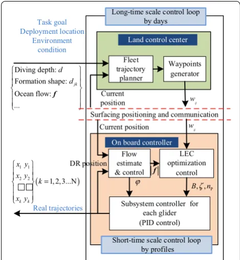
The coordinate of the HUG formation can be achieved by a multi-layer coordinate control system as shown in Figure 4. There are totally two control layers which are under control loop with different time scales. This con-trol system is not based on the dynamics of the glider.
The outer layer with long-time scale loop is integrated in the ground control center or the deck controller which can only work during communication when the glider surfaces. The function of outer layer is to plan the fleet trajectory and generate waypoints for each glider. The control software of Petrel-II can manipulate up to 10 glid-ers at the same time in one computer. Since each glider has sailing error and may be influenced by the ocean environment, the trajectory is re-planned every time loop for about 48/72 h by updating the current glider positions and the fresh task requirement (for adaptive glider sam-pling based on ocean model, the forecast period is 48/72 h [32]). The waypoints are updated to each glider by sur-facing communication. On the outer control layer, glid-ers update working status every profile and receive new command every long-time loop.
The inner layer with short time scale loop is integrated in the onboard controller inside each glider. This layer
receives the command waypoints from the outer layer and control the glider to move to the desired waypoints. Since endurance of the glider is very important for the long-term marine observation, a LEC (least energy con-sumption) algorithm is designed to minimize the energy cost in the glider motion. The distance between neighbor waypoints is calculated as the input of LEC and the opti-mal control variables are generated as the optimization output. The influence of ocean flow is considered by the controller. The glider gets its position every time it sur-faces and estimates the flow velocity by comparing the position with the dead-reckoned position (DK position) or that of the desired waypoint. The controller makes decision to decrease the influence of the flow by deter-mining the heading angle of the glider and outputs the flow speed into the LEC to obtain optimal control vari-ables. The onboard subsystem controller based on PID control will achieve the motion control under the optimal command. This control cycle loops every profile, so the inner layer is under a short-time loop by profiles.
3.2 Fleet Trajectory Planner
3.2.1 Multibody System Model Based on Kane’s Equation
The goal of the trajectory planning of multi-HUG is to generate optimal trajectories for each glider and mean-while shape the whole formation under given motion conditions (initial position, motion goal and obstacle location) and desired formation configuration (formation geometry). Artificial potential fields (APFs) method is adopted in the planner for its capabilities in steering the motion along the trajectory of global minimum potential energy. The multi-HUG formation is regarded as a vir-tual multibody system and for simplicity, the individual agent in the fleet is treated as a particle and is virtually connected with other agents in the multibody system. Motion simulation results of a three-glider fleet motion controlled by this method has been achieved in our early work (more details see Refs. [22, 33]).
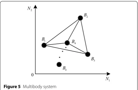
Kinematics: this study assumes it as a two-dimensional question since the desired trajectories of the gliders are only in horizontal plane. As an N-body system shown in Figure 5, the gliders are regarded as particles with full actuation. Bk represents the kth agent and all the bod-ies are fixed in the Cartesian reference frame which is denoted by the unit vector (N1, N2). Each body has two
degrees of freedom and the system has 2 N degrees of
freedom.
The position coordinates of the bodies can be chosen as the generalized coordinate, which is given by
where xkn (k = 1,…, N, n = 1, 2) represents the position coordinates of the kth body with respect to the inertial
(1)
ql=(x11,x12,. . .,xk1,xk2,. . .),
( )
1 1
2 2 1,2,3...N
k k
x y x y k
x y
=
Long-time scale control loop by days
Fleet trajectory
planner
Real trajectories
Land control center
Task goal Deployment location
Environment condition
On board controller Diving depth:
Formation shape: Ocean flow: ...
jk
d d
f
Waypoints generator
Subsystem controller for each glider (PID control)
LEC optimization
control Flow
estimate & control
Surfacing positioning and communication
Short-time scale control loop by profiles
ij
w
Current position
P , ,
Bζ n ϕ
ij
w
Current position
DR position
f
frame and n denotes the two axes of reference frame. The generalized speed can be expressed by
where x˙kn is the time derivative of xkn.
The partial velocity array is adopted to describe the kinematic characteristics of the multibody system, which can be obtained by
where vk is the velocity of the kth body in the inertial sys-tem, l = 1,…, 2 N represents the number of elements in the generalized coordinate, n, m = 1, 2 represent the two axes of the coordinate system, and is the velocity compo-nent of the agents.
Kinetics: The APFs are constructed for particular mis-sion requirement, ocean environment, and formation geometry. Attractive potential field [21] between the glid-ers and the task target can guide the formation to the goal area. Interactive potential field [34] between gliders can shape and maintain the formation geometry by pulling together or pushing away the neighboring vehicles when they are apart from each other or toward each other by a control distance. Repulsive potential field [35] between gliders and ocean obstacles is also necessary to avoid col-lision in the ocean environment. The three types of APFs are expressed by the following equations:
(2)
˙
ql=(x˙11,x˙12,. . .,x˙k1,x˙k2,. . .),
(3)
vklm= ∂vk ∂q˙l
=
∂ 2
n=1
˙ xknNn
∂q˙l ,
(4) Uattk =
0 0<
Rgk ≤dgoal, 1
2kaR2gk Rgk ≤dgoal,
(5) UI =
kI(12r2ij−d021n(rij)) 0<rij<d1, kI(12d12−d021n(d1)) rij≥d1,
(6) Urepk =
1
2kr(R1ok − 1 dobs)
2 0<R
ok≤dobs,
0 Rok>dobs,
where i, j, k are the ith, jth, kth bodies, i, j, k = 1…N, N is the total number of bodies, ka is the scalar attractive con-trol gain, kI is the scaling interactive control gain, kr is the scalar repulsive control gain, Rgk is the distance between the kth body and goal, Rok is the distance between the kth body and the effective obstacle, rij is the distance between the ith and jth bodies, d0 is the constant denoting the critical point between attraction and repulsion, d1 is the limited distance of interaction, dgoal is the equivalent radius of the attractive area, dobs is the distance of influence by the obstacles.
The potential forces generated by APFs are the negative gradients of potential fields:
where FAPF is the potential force and U is the artificial potential field. More derivation process of formulas can be obtained in Ref. [21]. Dissipative force is applied to individuals of the formation to achieve asymptotic stabil-ity at desired velocstabil-ity:
where FdissK is the dissipative force on the kth body, kdiss is
the scalar control gain, vd is the desired velocity of each glider.
Kane’s equation: The Kane’s equation has advantages in the construction of the dynamic equation with mini-mal sets of coordinates and complexity. The principle of Kane’s equation is that the sum of the generalized active force and the generalized inertia force equals to zero:
where Fl is the generalized active force and Fl∗ is the gen-eralized inertia force. Fl in the multi-HUG formation is the sum of the generalized active force corresponding to APFs force and dissipative force:
where Fal, Frl, FIl, and Fdisl is the generalized active force constructed by the attractive potential field, the repul-sion potential field, the interaction potential field and the dissipative control term, expressed in Eqs. (4)‒(8), respectively. See Ref. [36] for more details about the con-struction of Kane’s equation.
3.2.2 Waypoints Generator
The waypoints are chosen to steer each glider’s motion to the trajectory planned by the method presented in Section 3.2.1. There are two principles for converting trajectory to waypoints [18]. One is to space waypoints uniformly in time and the other is to let the waypoints subject to a maximum spacing constrain. Considering the practical operation, the second method is adopted to set a maximum space between two waypoints, which is
(7) FAPF = −∇U,
(8) FdissK = −kdiss(vk−vd),
(9)
Fl+Fl∗=0, l=1, 2,. . ., 2N,
(10) Fl =Fal+Frl+FIl+Fdisl, l=1, 2,. . ., 2N,
0
1
N
2
N
1
B
2
B
4
B
3
B
k
B
an optimization problem obtaining optimal points on the curve to minimize the distance function.
Let wki denotes the ith waypoint position of the kth body, k = 1,…, N and i = 1,…, p, p is the total number of the waypoints. The problem can be express as
where xkj is the jth calculated position on the planned trajectory of the kth body, j = 1,…, q, q is the number of the calculated position which is much larger than p, and
dr is the required distance between neighbor waypoints.
3.3 Optimal Onboard Control Based on LEC 3.3.1 Least Energy Consumption Algorithm (LEC)
Model: since the Petrel-II glider is an under actuated system with the compound motion in horizontal plane, it is difficult to analyze the energy consumption of the
system based on the motion dynamic model [37]. The
method [29, 30, 38] that finds the relationship between the motion parameters (gliding angle, diving depth, etc.) and the energy cost of the subsystem by analyzing the glider operation principle and control flow, can simplify the complication of the question and give a practical expression. In this article, based on the main concept in the Refs. [29, 30, 38], an energy consumption model of the screw propeller driven hybrid underwater glider is established under the following assumptions:
(1) The question is assumed only in the vertical plane for the vertical motion (diving and rising) of glider cost the major power.
(2) The energy cost is considered under the steady glid-ing motion. It is assumed under the force balance condi-tion with drag force D, lift force L, net buoyancy force B
and screw propeller driven force P (exiting under hybrid motion condition) acted on the glider.
The force diagram of the glider under steady gliding balance is shown in Figure 6. Let the scalars D, L, B and P represent the magnitude of the force D, L, B and P, respectively. When considering the propulsion force P, the attack angle α is simplified to be zero, and the balance equations of the system can be given by
where α and ζ are the attack angle and the gliding angle of
the glider, respectively, and ε is the condition coefficient
given by
The drag force and lift force are related to the gliding speed V and the attack angle α. The propulsion of screw
(11) minf(xkj)= ||xkj−wk(i−1)||2 −dr,
(12)
L=Bcosζ,
D=Bsinζ +εP,
(13) ε=
0, under gliding mode, 1, under hybird mode.
propeller is related to its rotate speed nP, its diameter DP and the seawater density ρ. The three forces can be expressed by
where the KD0, KD, KL0, and KL, are the coefficients of drag force and lift force, respectively. KP is coefficient of the pro-pulsion which can be obtained by the screw propeller atlas. The gliding speed is a function of the variables B, nP and ζ .
And the motion time of the distance S between neighbor waypoints can be obtained by
The energy consumed during the glider motion can be divided into two classes [38]: the energy cost by the con-tinuous working units (the control unit, part of sensors and screw propeller), which is related to gliding time,
symbolled by Et and the energy consumed by motion
driven units which is related to the number of working profiles, symbolled by En.
where Et = Pt·t, En=n·(Eh+Em),Pt is the total power
of the continuous working units, n is the number of the gliding profiles.
And Eh is energy cost by buoyancy driven unit, which is considered as the consumption of the hydraulic system when glider dives and rises. Em is the energy cost by the attitude adjusting unit, which is considered as the con-sumption of the motor driving the battery movement.
where Pv is the power of the magnetic valve, Pp0 and kp are coefficients of the hydraulic pump which are related to its working depth (i.e., diving depth) d, g is the accel-eration of gravity, qv and qp are the fluxes of the magnetic
(14)
D=�
KD0+KDα2
�
V2,
L=(KL0+KLα)V2, P=KPρDP4n2P,
(15)
t= S
Vcosζ.
(16) E =Et+En,
(17) Eh=n·VB·Ph=n·
2B ρg ·(
Pv qv
+Pp0+kpd
qp ),
(18) Em=n·
4Pmr vm
,
α θ
ζ
y B
D L
P
v
x
valve and hydraulic pump, respectively. ρ is the seawater
density which is related to the temperature, pressure and salinity at the related position and depth undersea, and it is taken as a constant for simplicity in this study. Pm is the power of the attitude adjusting motor, vm is the speed of the moving package and r is the movement of the pack-age from the equilibrium position, which is determined by the pitch angle:
where pitch angle is assumed to be equal to the gliding angle for the attack angle is small. M and m are masses of glider and moving package respectively, and h is the metacentric height.
Algorithm: the total energy consumption is obtained by Eqs. (16)‒(19), from which we can analyze the relation-ship between the energy, the motion parameters and the control variables. The time-related energy is determined by the required distance between neighbor waypoints S, the gliding angle ζ and the gliding speed V which is
fur-ther determined by the net buoyancy B and the rotate
rate of the screw propeller nP. The profile-related energy is determined by the gliding angle ζ, the number of pro-files n, the diving depth d and the net buoyancy B. Thus, the total energy consumption function can be expressed by
Endurance is important for the glider to achieve long term ocean observation. The question is how to make the battery on the glider sustain as long as possible. A low energy cost optimization can be designed to choose the optimal variables to minimize the total energy cost based on the energy consumption function when given the required conditions S and d. Thus, the optimization problem can be expressed by
where Bo, ζo and nPo are the optimal variables, Bmin and Bmax represent the ability of the net buoyancy deter-mined by the design volume of oil tank, and ζmin, and
ζmax are the minimum value and maximum value of the
gliding angle which is determined by the intersection of the design attitude adjusting range and the stable gliding
(19) r= M·h
m ·tanζ,
(20) E =f(S,d,B,nP,n,ζ ).
(21)
minf(S,d,B,nP,n,ζ ),
s.t.Bmin ≤B ≤Bmax,
ζmin ≤ ζ ≤ζmax, nPmin ≤ nP ≤nPmax,
n= �
S·tanζ
2d �
,
condition. nPmin and nPmax are the rotate speed extreme values of normally glider operation. ⌈•⌉ is to round up
the value to make sure that the glider can arrive at the desired surfacing position.
3.3.2 Flow Estimate and Motion Correction
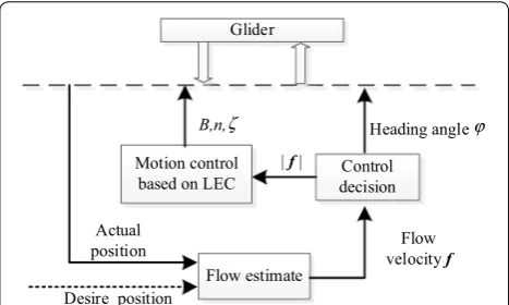
The existence of ocean flow (ocean current) always influ-ences the trajectory of the glider since the speed of the glider in horizontal plane is generally less than 0.4 m/s which has the same magnitude with the speed of the flow. A control scenario is designed to control the glider motion with the existence of ocean flow, shown in Figure 7.
The controller first estimates the velocity of ocean flow by the actual position and the desired position during every time the glider surfaces. Then the controller makes decision to determine the heading angle of the next motion and outputs the estimated speed into the LEC module. The optimal control variables can be obtained with the existence of ocean flow.
Flow estimate: The actual and the desired horizontal positions of glider at current surfacing time t are denoted by r(t) and r′(t), respectively. The average flow velocity of the last profile can be estimated by
where t is the motion period of the last profile and the
surfacing time is assumed to be contained in the period. Compared with the ocean model based forecast, this method is much easier and does not need larger amount of precise sensor data. It is suitable to integrate into the onboard control system.
Heading angle determination: In order to keep the glider moving to the next waypoint, the direction of the resultant velocity of the desired glider velocity and the flow velocity should be on the connection of the current position and the next waypoint. When the glider is capa-ble to move along the desired direction, the heading angle should be set same with the angle of the desired glider velocity. Otherwise, when the ocean flow is too strong for the glider to move on the resultant velocity direction, the heading angle should be set opposite to that of the ocean
(22) ft=
r(t)−r(t)
�t ,
flow velocity. The criteria that tests whether the glider can move along desired direction is presented in Ref. [39].
LEC with ocean flow: Since ocean flow influences the speed of the glider, the motion time in the energy con-sumption model is changed by flow speed. The glider velocity relative to ground is the vector sum of the flow velocity and the water–referenced velocity [29].
The motion time of the distance S between neighbor
waypoints can be obtained by
4 Simulation and Primary Sea Experiment
In order to verify the availability of the coordinate control algorithm, an actual deployment of three Petrel-II glid-ers has been carried out in the South China Sea. In this section, a simulation test of optimal control base on LEC (see Section 3.3.1) is also presented to show the necessity of the method.
4.1 Simulation Test of Optimal Control Based on LEC
The Petrel-II glider is taken as the simulation object. The energy consumption model expressed by Eqs. (16)‒(19) is programmed in MATLAB to implement the simula-tion. The hydrodynamic coefficients and the subsystem parameters of Petrel-II involving in the model are listed in Table 2. For simplicity, the depth density value of 1000 m is taken as a constant seawater density, which is obtained by fitting the experiments data [40] of Petrel-II deployed in the South China Sea.
The distance between neighbor waypoints is set to be 6 km in the simulation. Figure 8 shows the regularity of
the energy consumption with the net buoyancy B,
div-ing depth d and the number of profiles n. The energy cost increases along with the increase of the diving depth as shown in Figure 8. The energy cost by one-profile glid-ing is lower than two-profile glidglid-ing, and the one-profile energy cost increases faster than the two-profiles energy cost with the increase of the diving depth, which illus-trates that the number of the profiles should be less in the practical glider operation. And the energy cost decreases to a minimum value then increases along with the increase of the net buoyancy. This implies that the LEC method is necessary to obtain an optimal net buoyancy which minimize the energy consumption.
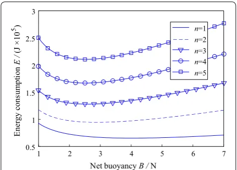
There are maximally five profiles calculated by the LEC constrained by the gliding angle range by setting the desired diving depth to 1000 m and the waypoints dis-tance to 6 km. The results are shown in Figure 9, and the comparison of five different numbers of gliding profiles
(23)
V′=f +Vglider.
(24)
t= S
||V′||cosζ.
Flow estimate
Control decision Motion control
based on LEC
Actual position
Desire position
Flow velocity f
| f|
ϕ B,n,
Glider
Heading angle ζ
shows the optimal net buoyancy locating on the curve of one-profile gliding.
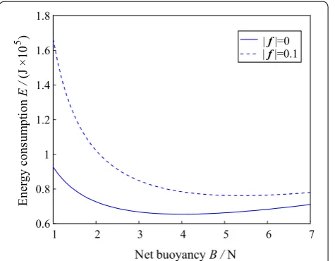
Figure 10 shows the energy consumed without and
with the existence of the ocean flow by setting the dis-tance to 6 km and the diving depth 1000 m under one-profile gliding, respectively. The blue solid line represents the regulation without ocean flow and the blue dash line represents the result with a flow at speed of 0.1 m/s. It shows that the optimal net buoyancy value and the energy value get bigger when ocean flow exists. The value of the optimal net buoyancy and minimum energy can be obtained by the Algorithm 1. The optimal net buoyancy
is 4.0 N and 5.4 N respectively. And the corresponding minimum energy is 6.5440 × 10⁴ J and 7.6193 × 10⁴ J. This illustrates that it costs more for glider to move to the desired waypoint when ocean flow existing and it also implies that the high net buoyancy regulating ability is important in the glider system designed to operate under ocean flow.
Figure 11 shows the energy consumption under the
hybrid motion mode with the same motion conditions of S and d. The result shows that one-profile motion costs more energy than two-profile motion. The regula-tion is influenced by the existence of the propeller pro-pulsion compared with Figures 8‒10. The energy cost by hybrid motion is much larger than in the unmixed glid-ing, which illustrates that the major energy is consumed by the motor of screw propeller and in order to ensure long term task, the hybrid mode should be applied only when fast motion is necessary. Based on LEC, the opti-mal rotate speed is 1000 r/min, the optiopti-mal net buoyancy is 7 N and the minimum energy is 3.2877 × 10⁵ J .
4.2 Actual Deployment in the South China Sea
A fleet of three Petrel gliders, referred to as EG03, EG04 and EG05, was deployed in the South China Sea in Sep-tember 2014. The goal of the experiment was to test the coordinate control algorithms delivered in Section 3.
Figure 12 shows the mission area where the three glid-ers move as a triangle to two targets in order. The yellow dash line around targets is the effective area with a radius of 5 km. The two target positions of EG03, as a leader of the fleet, are:
T1(18◦11′N, 111◦50′E),
T2(18◦10′N, 111◦58′E). Table 2 Parameters and augments of Petrel‑II
Parameter Value
Lift coefficient KL0, KL − 0.5, 381.73
Drag coefficient KD0, KD 7.65, 357.97
Mass of Petrel‑II M/kg 65
Mass of battery package m/kg 18
Metacentric height h/m 0.04
Diameter of screw propeller DP/m 0.08
Seawater density ρ /(kg/m3) 1030
Power of pitch motor Pm/W 10
Power of magnetic valve Pv/W 5
Power of pump (surface) Pp0/W 22.4
Coefficient of pump power k/(W·m) 0.032
Coefficient of screw propulsion kP 0.023
Flux of pump qp/(m3/s) 1.3 × 10⁻⁶
Flux of magnetic valve qv/(m3/s) 2 × 10⁻⁵
Net buoyancy range B/N [1, 7]
Gliding angle range ζ /(°) [10, 60]
Rotate rate of screw propeller nP/(r/min) [200, 1000]
4 8 6
1000 8
6 10
4 12
500 2
0 0
5 6 7 8 9 10 11
n=2
n=1
En
er
gy cons
um
pt
ion
Net buoyan cy B / N
E
/
(J
×
)
4
10
Figure 8 Regularity of the energy consumption with the net buoy‑
ancy B, diving depth d and the number of profiles n
1 2 3 4 5 6 7
Net buoyancy B / N
0.5 1 1.5 2 2.5 3
n=1
n=2
n=3
n=4
n=5
5
En
er
gy cons
um
pt
ion
E
/
(J
×
10
)
The start position of EG03, EG04 and EG05 are:
The geometry of the formation is constrained by the interactive distance between EG03 and EG04, EG03 and EG05, EG04 and EG05 which are 10 km, 7 km and 10 km, respectively.
The trajectories of the gliders were generated by the fleet trajectory planner which shaped the desire forma-tion geometry and achieved the sailing goals. Generally,
P1
18◦18′59′′N, 111◦35′26′′E
,
P2
18◦23′19′′N, 111◦31′55′′E
,
P318◦18′54′′N, 111◦31′42′′E.
1 2 3 4 5 6 7
0.6 0.8 1 1.2 1.4 1.6 1.8
| f |=0
Net buoyancy B / N
5
En
er
gy cons
um
pt
ion
E
/
(J
×
10
)
| f|=0.1
Figure 10 Energy consumption of 1000 m diving depth under ocean flow
P
n
2 8
4 200
6
6 8
400 10 12
4 14
600 16
2 800
0 1000
4 5 6 7 8 9 10 11 12 13 14
En
er
gy cons
um
pt
ion
E
/
(J
×
)
5
10 n=2
n=1
1
r min⋅ −
Figure 11 Energy consumption of 1000 m diving depth under hybrid motion mode
Figure 12 Mission area of the sea trial
550 560 570 580 590 600 605 2000
2005 2010 2015 2020 2025 2030 2035 2040
EG03 EG04 EG05
Position coordinate x / km
Po
si
tion
co
or
di
na
te
y
/
km
Figure 13 Trajectory of the formation generated by the fleet trajec‑ tory planner
111.5 111.6 111.7 111.8 111.9 112
Latitude Lat / ( ° N)
18.1 18.15
18.2 18.25
18.3 18.35
18.4 18.45
EG03 EG04 EG05
Longi
tu
de
Lo
n
/
( °
E)
0 10 0
200 400 600 800
0 10
0 200 400 600 800
0 10
0 200 400 600 800
900 900 900
17 17 17
Di
vi
ng de
pt
h of
EG
03
d
/
m
The ordinal of profiles n The ordinal of profiles n The ordinal of profiles n
Di
vi
ng de
pt
h of
EG
04
d
/
m
Di
vi
ng de
pt
h of
EG
05
d
/
m
a
b
c
Figure 15 Diving depth of each glider
0 10
0 1 2 3 4 5 6
0 10
0 1 2 3 4 5 6
0 10
0 1 2 3 4 5 6
17 17 17
Ne
t buoyancy of
EG
03
B
/
N
The ordinal of profiles n
Ne
t buoyancy of
EG
04
B
/
N
Ne
t buoyancy of
EG
05
B
/
N
The ordinal of profiles n The ordinal of profiles n
a
b
c
Figure 16 Net buoyancy of each glider
10 0
20 40 60 80 100 120 140
10 0
20 40 60 80 100 120
10 0
20 40 60 80 100 120 140
17 7
1 7
1 The ordinal of profiles n
He
adi
ng angl
e of
EG
04
/
(°
)
H
eadi
ng angl
e of
EG
05
/
(°
)
ζ ζ
The ordinal of profiles n The ordinal of profiles n
He
adi
ng angl
e of
EG
03
/
(°
)
ζ
a
b
c
the trajectories are renewed every two or three days by updating current position of the glider, the environment information and current task arrangement. As this exper-iment was a short-term test for only three days, the tra-jectories were calculated once when the task began. The
planned trajectories are shown in Figure 13, in which the coordinates of the gliders are converted to the earth coordinates from the latitude–longitude coordinates. The glider was commanded to dive to average depth of 800 m every profile. The waypoints of the leader glider EG03 were chosen by the waypoints generator by giving the desired distance d equal to 3 km with a truncation error of 0.3 km. The waypoints of EG04 and EG05 were set by the position related to the corresponding moment of every EG03 waypoint. The waypoints near the two desire positions were alternated by the latter. The small red cycle, red * and red × in Figure 13 represent the planned waypoints of EG03, EG04 and EG05, respectively.
The total number of profiles, the net buoyancy of every profile and the heading angle after every surfacing was determined by the onboard controller considering the energy consumption and the ocean flow environ-ment. In this case, each glider was desired to run 15 pro-files during the mission. Specifically, an addition profile before the desired motion is necessary to test the status of each components onboard and calibrate the control coefficients referenced by the sea environment, which is always set to dive less than 100 m. The actual fleet trajec-tory is shown in Figure 14. Compared with the planned trajectory shown in Figure 13, the actual fleet trajectory keeps the path shape and formation geometry basically. The surface locations of each glider float around the pre-set waypoints. The position errors are mainly caused by the uncertainties of ocean environment, the errors of the flow estimation, the errors of the GPS location, the laten-cies of communication and the errors of control system.
Figure 15 records the moving process of each glider in vertical plane. The diving depth of each glider is detected by the onboard pressure sensor. The total number of
0 5 10 15 17
The ordinal of profiles n
0 5 10
0 5 10 15
The ordinal of profiles n
22 23 24
0 5 10 15 17
The ordinal of profiles n
0 5 10
0 5 10 15
The ordinal of profiles n
22 23 24
0 5 10 15 17
0 5 10
0 5 10 15
22 f c Es Ea Es Ea Es Ea 23 24 EG
04 ene. con.
E / ( J × ) 4 10
The ordinal of profiles n The ordinal of profiles n
d a
e b
EG
03 ene. con.
E / ( J × ) 4 10 EG
05 ene. con.
E / ( J × ) 4 10 Di ff er ence / (% ) ε Di ff er ence / (% ) ε Di ff er ence / (% ) ε
Figure 18 Comparison of simulated energy consumption and actual energy consumption of each glider
0 5 10 15
0 0.5 1 1.5 2 2.5
0 5 10 15
0.2 0.4 0.6 0.8 1 1.2 1.4 1.6
0 5 10 15
0.2 0.4 0.6 0.8 1 1.2 1.4 1.6 1.8 2
The ordinal of profiles n The ordinal of profiles n The ordinal of profiles n
Tr aj ect or y er ro r of EG 05
/ kme
d Tr aj ec to ry e rro r of EG 04
/ kme
d Tr aj ec to ry e rro r of EG 03
/ kme
d
a
b
c
diving profiles is 16 with an additional test profile at the depth of 50 m. And the depth of other profiles is mainly 800 m with an error range of [− 10, 10] m. The average net buoyancy of each profile is calculated by the records of the residual oil volume in the inner ballast, as shown in Figure 16, which is larger than the optimal value shown in Figures 9, 10. This is caused by the existence of ocean flow and the errors of the onboard control system. The actual control heading angle is shown in Figure 17. The sharp changes of the heading angle happened in the inflection points of the trajectory and the area that the flow speed might be higher than the through-water speed of the glider.
The minimum energy consumption of each profile was calculated by choosing optimal control variables before each diving. The actual energy consumption was obtained by the real-time onboard records of the battery volt-age and current. Figure 18 gives a comparison between the simulation results and actual energy consumption. In Figures 18(a)‒(c), the yellow bar and blue bar repre-sent the actual profile energy cost Ea and the simulated energy cost Es. The average simulated energy cost of EG03, EG04 and EG05 is 6.6852 × 10⁴ J, 6.6880 × 10⁴ J and 6.6862 × 10⁴ J. The corresponding actual energy con-sumption of each glider is 8.6718 × 10⁴ J, 8.6716 × 10⁴ J and 8.6525 × 10⁴ J.
Figures 18(d)‒(f) shows the percentage difference
between the two quantities, which is in the range of [22%, 24%] basically. The difference in Figure 18 is mainly caused by the limitation of calculation model which con-sidered only vertical motion consumption and the errors of onboard control.
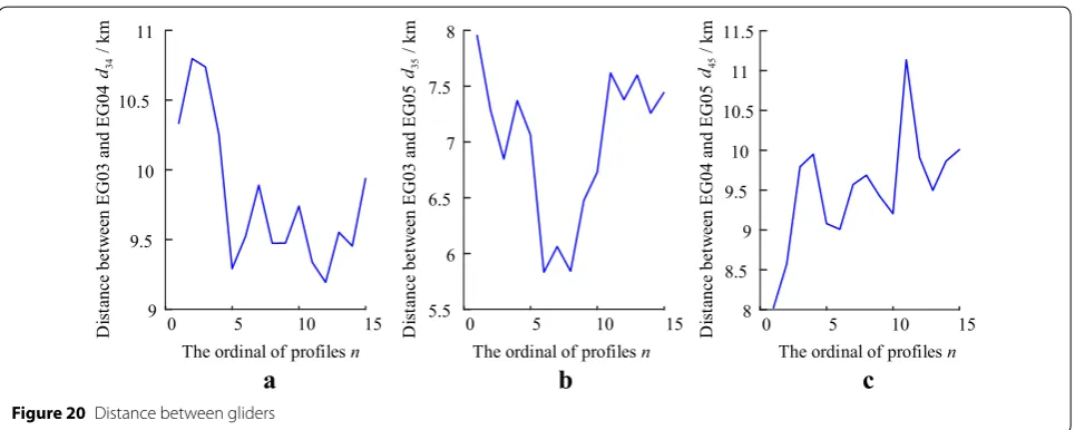
Trajectory error of each glider and the distance between gliders are adopted to evaluate the performance of the fleet controlled by the method presented in this
paper. The results are shown in Figures 19, 20. The tra-jectory error of each profile is defined by the distance between the desired position and the actual surfacing position. The maximum error of each glider is 2.41 km, 1.3 km, 1.9 km respectively, as shown in Figure 19. The distance between gliders at each surfacing can help to evaluate the geometry maintaining performance of the formation. As shown in Figure 20, the distance fluctuates around the desired distance with a floating range of less than 2 km. The results prove that the fleet can basically move along the desire trajectory and keep the desired formation shape during the sea experiment. The higher trajectory error might be caused by the low estimate pre-cision of the ocean flow, low control accuracy and uncer-tainty error. This implies that the regional ocean model which can forecast the ocean environment might be nec-essary in the coordinate control of multi-HUG formation.
5 Conclusions
(1) A multi-layer coordinate control strategy is pro-posed to achieve the coordinate control, motion optimization of Multi–HUG formation.
(2) An energy consumption model is constructed for HUGs with the consideration of hybrid motion. The Least Energy Consumption (LEC) algorithm is proposed to minimize the motion energy cost with consideration of ocean flow existence.
(3) The regularities of HUG energy consumption with motion variables is studied by simulation. The results show that the number of profiles is better to be less to extant endurance and the energy con-sumption under ocean flow is larger than the situ-ation without flow existence, which need larger net buoyancy. It also suggests the propeller costs much more energy than other components under
0 5 10 15
9 9.5
10 10.5
11
0 5 10 15
5.5 6 6.5
7 7.5
8
0 5 10 15
8 8.5
9 9.5
10 10.5
11 11.5
The ordinal of profiles n The ordinal of profiles n The ordinal of profiles n
Di
st
ance be
tw
een
EG
03 and
EG
04
/ km
Di
st
ance be
tw
een
EG
03 and
EG
05
/ km
Di
st
ance be
tw
een
EG
04 and
EG
05
/ km
a
b
c
34
d d35 d45
hybrid motion which need the largest net buoy-ancy to save energy.
(4) A primary sea experiment of three Petrel-II gliders is achieved in the South China Sea. The actual fleet trajectory is similar with the planned path and the formation geometry fits the shape request. The tra-jectory error is less than 2.5 km and the formation shape error is less than 2 km which meet the preset task request. The results verify the feasibility of the multi-layer control strategy and the effect of LEC algorithm.
(5) The modeled energy consumption is about 76%‒78% of the actual energy consumption of each glider. This implies the model can basically describe the energy cost of HUG. The future work could be drawn in more precise model considering three-dimensional motion.
Authors’ contributions
DYX carried out the dynamic modeling studies, and drafted the manuscript. ZLW carried out the control system design. YHW carried out the sea trials of the Petrel underwater gliders, participated in the analyzing of the test data and the design of the Petrel underwater glider. SXW carried out the design of the Petrel underwater glider, participated in the analyzing of the test data. All authors read and approved the final manuscript.
Author details
1 Key Laboratory of Mechanism Theory and Equipment Design of Ministry of Education, Tianjin University, Tianjin 300072, China. 2 School of Mechanical Engineering, Tianjin University, Tianjin 300072, China. 3 The Joint Laboratory of Ocean Observing and Detecting, Qingdao National Laboratory for Marine Science and Technology, Qingdao 266237, China.
Authors’ Information
Dong‑Yang Xue, born in 1987, is currently a PhD candidate at School of Mechanical Engineering, Tianjin University, China. She received her master degree from Northeastern University, China, in 2011. She received her bachelor degree from Northeastern University, China, in 2009. Her research interests include autonomous underwater vehicle and multiple agents control.
Zhi‑Liang Wu is currently an associate professor at School of Mechanical Engineering, Tianjin University, China. Her research interests focus on coordina‑ tion of mobile autonomous agents.
Yan‑Hui Wang born in 1979, received his bachelor, master and PhD degrees on mechanical engineering from Tianjin University, China, where he is currently a professor at School of Mechanical Engineering. He has been involved in the research of various underwater vehicles.
Shu‑Xin Wang born in 1966, received his bachelor degree on mechanical engineering from Hebei University of Technology, China, in 1987 and master and PhD degrees on mechanical engineering from Tianjin University, China. He is currently a professor at Tianjin University, China and has been active in various aspects of the research and design of ocean vehicles since 2000.
Acknowledgements
Supported by National Key R&D Plan of China (Grant No. 2016YFC0301100), National Natural Science Foundation of China (Grant Nos. 51475319, 51575736, 41527901), and Aoshan Talents Program of Qingdao National Labo‑ ratory for Marine Science and Technology, China.
Competing interests
The authors declare that they have no competing interests.
Ethics approval and consent to participate Not applicable.
Publisher’s Note
Springer Nature remains neutral with regard to jurisdictional claims in pub‑ lished maps and institutional affiliations.
Received: 11 March 2016 Accepted: 14 January 2018
References
1. C C Eriksen, T J Osse, R D Light, et al. Seaglider: a long‑range autonomous underwater vehicle for oceanographic research. IEEE Journal of Oceanic Engineering, 2001, 26(4): 424–436.
2. D C Webb, P J Simonetti, C P Jones. SLOCUM: an underwater glider pro‑ pelled by environmental energy. IEEE Journal of Oceanic Engineering, 2001, 26(4): 447–452.
3. J Sherman, R E Davis, W B Owens, et al. The autonomous underwater glider “Spray”. IEEE Journal of Oceanic Engineering, 2001, 26(4): 437–446. 4. G Marani, S K Choi, J Yuh. Underwater autonomous manipulation for
intervention missions AUVs. Ocean Engineering, 2009, 36(1): 15–23. 5. D L Orange, J Yun, N Maher, et al. Tracking California seafloor seeps with
bathymetry, backscatter and ROVs. Continental Shelf Research, 2002, 22(16): 2273–2290.
6. Z J Yu, Z Q Zheng, X G Yang, et al. Dynamic analysis of propulsion mecha‑ nism directly driven by wave energy for marine mobile buoy. Chinese Journal of Mechanical Engineering, 2016, 29(4): 710–715.
7. X Q Zhu, W S Yoo. Numerical modeling of a spherical buoy moored by a cable in three dimensions. Chinese Journal of Mechanical Engineering, 2016, 29(3): 588–597.
8. B Claus, R Bachmayer, C D Williams. Development of an auxiliary propul‑ sion module for an autonomous underwater glider. Journal of Engineering for the Maritime Environment, 2010, 224(4): 255–266.
9. A Alvarez, A Caffaz, A Caiti, et al. Folaga: a low‑cost autonomous under‑ water vehicle combining glider and AUV capabilities. Ocean Engineering, 2009, 36(1): 24–38.
10. F Liu, Y H Wang, S X Wang. Development of the hybrid underwater glider Petrel‑II. Sea Technology, 2014, 55(4): 51–54.
11. S X Wang, F Liu, S Shao, et al. Dynamic modeling of hybrid underwater glider based on the theory of differential geometry and sea trails. Journal of Mechanical Engineering, 2014, 50(2): 19–27. (in Chinese).
12. Z E Chen, J C Yu, A Q Zhang, et al. Design and analysis of folding propul‑ sion mechanism for hybrid‑driven underwater gliders. Ocean Engineering, 2016, 119: 125–134.
13. M P Stephanie. Autonomous & adaptive oceanographic feature tracking on board autonomous underwater vehicles. American: MIT and WHOI Doctor, 2015.
14. N E Leonard, D A Paley, R E Davis, et al. Coordinated control of an under‑ water glider fleet in an adaptive ocean sampling field experiment in Monterey bay. Journal of Field Robotics, 2010, 27(6): 718–740.
15. J Zhao, C M Hu, J M Lenes, et al. Three‑dimensional structure of a Karenia brevis bloom: observations from gliders, satellites, and field measure‑ ments. Harmful Algae, 2013, 29(4): 22–30.
16. A Alvarez, J Chiggiato, K Schroeder. Mapping sub‑surface geostrophic currents from altimetry and a fleet of gliders. Deep‑Sea Research Part I‑Oceanographic Research Papers, 2013, 74: 115–129.
17. X L Liang, W C Wu, D S Chang, et al. Real‑time modelling of tidal current for navigating underwater glider sensing networks. 3rd International Con-ference on Ambient Systems, Networks and Technologies/9th International Conference on Mobile Web Information Systems. Niagara Falls, CANADA, August 27–29, 2012. Procedia Computer Science, 2012, 10: 1121–1126. 18. D A Paley, F M Zhang, N E Leonard. Cooperative control for ocean sam‑ pling: the glider coordinated control system. IEEE Transactions on Control Systems Technology, 2008, 16(4): 735–744.
19. T B Curtin, J G Bellingham, J Catipovic, et al. Autonomous oceanographic sampling networks. Oceanography, 1993, 6(3): 86–94.
20. B Das, B Subudhi, B B Pati. Cooperative control coordination of a team of underwater vehicles with communication constraints. Transactions of the Institute of Measurement and Control, 2016, 38(4): 463–481.
Orlando, Florida, December 04‑07, 2001. IEEE Conference on Decision and Control–Proceedings, 2001: 2968–2974.
22. Y Yang, S X Wang, Z L Wu, et al. Motion planning for multi‑hug formation in an environment with obstacles. Ocean Engineering, 2011, 38(17–18): 2262–2269.
23. S X Ren, Y Zhang, C Z Chen. Negotiation of the multi‑underwater glider system. First international conference on innovative computing, information and control, Beijing, China, August 30–September 01, 2006. ICICIC 2006, 2006, 2: 138–141.
24. X Qi, L J Zhang, J M Zhao. Adaptive path following and coordinated con‑ trol of autonomous underwater vehicles. Proceedings of the 33rd Chinese Control Conference, Nanjing, China, July 28–30, 2014. USA: Piscataway, NJ, IEEE, 2014: 2127–2132.
25. D B Tang, M Dai. Energy‑efficient approach to minimizing the energy consumption in an extended job‑shop scheduling problem. Chinese Journal of Mechanical Engineering, 2015, 28(5): 1048–1055.
26. Z S Ma, Y H Wang, S X Wang, et al. Ocean thermal energy harvesting with phase change material for underwater glider. Applied Energy, 2016, 178: 557–566.
27. M Brito, D Smeed. Underwater glider reliability and implications for sur‑ vey design. Journal of Atmospheric and Oceanic Technology, 2014, 31(12): 2858–2870.
28. D Rao, S B Williams. Large‑scale path planning for underwater gliders in ocean current. Australasian Conference on Robotics and Automation(ACRA), Sydney, Australia, December 2–4, 2009. Australia: Australian Robotics and Automation Association Inc., 2009: 1–8.
29. J C Yu, F M Zhang, A Q Zhang, et al. Motion parameter optimization and sensor scheduling for the sea‑wing underwater glider. IEEE Journal of Oceanic Engineering, 2013, 38(2): 243–254.
30. Y J Zhou, J C Yu, X H Wang. Path planning method of underwater glider based on energy consumption model in current environment. Intelligent
Robotics and Applications. 7th International Conference, Guangzhou, China, December 17–20, 2014. Switzerland: Springer International Publishing, 2014: 142–152.
31. F Liu. System design and motion behavior analysis of the hybrid underwater glider. Tianjin: Tianjin University, 2014. (in Chinese).
32. J D Han, Z Q Zhu, Z Y Jiang, et al. Simple PID parameter turning method based on outputs of the closed loop system. Chinese Journal of Mechani-cal Engineering, 2016, 29(3): 465–474.
33. B Mourre, A Alvarez. Benefit assessment of glider adaptive sampling in Ligurian Sea. Deep‑Sea Research Part I‑Oceanographic Research Papers, 2012, 68(5): 68–78.
34. P Bhatta, E Fiorelli, F Lekien, et al. Coordination of an underwater glider fleet for adaptive ocean sampling. Proceedings IARP International Work-shop on Underwater Robotics, Genova, Italy, 2005: 61–69.
35. S S Ge, Y J Cui. Dynamic motion planning for mobile robots using poten‑ tial field method. Autonomous Robots, 2002, 13(3): 207–222.
36. D Y Xue, Z L Wu, S X Wang. Dynamical analysis of autonomous underwa‑ ter glider formation with environmental uncertainties. IUTAM Symposium on Dynamical Analysis of Multibody Systems with Design Uncertainties, Stuttgart, GERMANY, June 10–13, 2014. Netherlands: Elsevier B.V., 2015, 13: 108–117.
37. S X Wang, X J Sun, Y H Wang, et al. Dynamic modeling and motion simulation for a winged hybrid‑driven underwater glider. China Ocean Engineering, 2011, 25(1): 97–112.
38. X K Zhu. Methods research of underwater gliders for ocean sampling. Shen‑ yang: Chinese Academy of Sciences, 2011. (in Chinese).
39. D Chang, F M Zhang, C R Edwards. Real‑time guidance of underwater gliders assisted by predictive ocean models. Journal of Atmospheric and Oceanic Technology, 2015, 32(2): 562–578.