R E S E A R C H
Open Access
An evolutionary feature synthesis approach for
content-based audio retrieval
Toni Mäkinen
*, Serkan Kiranyaz, Jenni Raitoharju and Moncef Gabbouj
Abstract
A vast amount of audio features have been proposed in the literature to characterize thecontentof audio signals. In order to overcome specific problems related to the existing features (such as lack of discriminative power), as well as to reduce the need for manual feature selection, in this article, we propose an evolutionary featuresynthesis
technique with abuilt-infeature selection scheme. The proposed synthesis process searches for optimal linear/ nonlinearoperatorsand featureweightsfrom a pre-defined multi-dimensional search space to generate a highly discriminative set of new (artificial) features. The evolutionary search process is based on a stochastic optimization approach in which a multi-dimensionalparticle swarm optimizationalgorithm, along withfractional global best formationand heterogeneous particle behavior techniques, is applied. Unlike many existing feature generation approaches, the dimensionality of the synthesized feature vector is also searched and optimized within a set range in order to better meet the varying requirements set by many practical applications and classifiers. The new features generated by the proposed synthesis approach are compared with typical low-level audio features in several classification and retrieval tasks. The results demonstrate a clear improvement of up to 15–20% in average retrieval performance. Moreover, the proposed synthesis technique surpasses the synthesis performance of evolutionaryartificial neural networks, exhibiting a considerable capability to accurately distinguish among different audio classes.
Keywords:Content-based retrieval, Evolutionary computation, Particle swarm optimization, Feature selection, Feature generation
Introduction
Due to the drastically increased amount of multimedia data available in the Internet and in various public and personal databases, the development of efficient index-ing and retrieval methods for large multimedia databases has become a widely studied research topic. Scientific fields, such as digital signal processing (DSP) and com-puter science (particularlymachine learning), provide ef-ficient and mathematically well-defined methods for data mining and knowledge discovery from specific observations or databases [1]. One of the major research foci in the field is concentrated around content-based classification using supervised learning methods. In these, a dataset together with its perceived class labels, known as“ground truth,” is used to train a classifier, so that it can learn to discriminate among the individual
classes in the training dataset. This enables the classifier to classify new, previously unseen data items with a cer-tain degree of accuracy. Once successful such methods can be applied to several application areas, such as advanced database browsing, query-by-example retrieval, highlight-spotting from movies and/or sport events, speaker recognition, and so on.
In general, whenever machine learning techniques are to be applied to data classification or clustering tasks, certainfeaturesneed to be extracted from the data. The features can be numerical or nominal scalars or vectors describing specific characteristics of the data such as, in the case of audio signals, tonality or fundamental fre-quency (FF). Because the data classification and mining methods are strongly dependent on the extracted fea-tures, their quality and discriminative capability have an obvious influence on overall classification performance. Unfortunately, despite the enormous number of different audio feature extraction methods available in the * Correspondence:[email protected]
Department of Signal Processing, Tampere University of Technology, P.O. Box 553, Tampere, Finland
literature, the features have limitations and drawbacks in describing the data content, so that the current audio classifiers cannot really compete with the human auditory perception system. As will be shortly reviewed, such a lack of semantic representation, the “semantic gap,” has led to developing several promising techniques to obtain more power of discrimination from the extracted low-level features. The related work in this field is presented in the following section, which focuses on the two most important feature enhancement methods in the literature, feature selectionandfeature synthesis(also known as fea-turegeneration/construction/transformation).
Related work
Generally in machine learning, it is desirable to work with low-dimensional feature vectors (FVs) to reduce computational complexity, and also to avoid the so-called curse of dimensionality phenomenon [2], which basically states that in high-dimensional representations the available data become too sparse for any decent stat-istical or structural analysis. In a feature selection scheme, the FV dimensionality is lowered by selectively choosing an expressive and compact set of features among a possibly much larger original set. Evolutionary algorithms, such asgenetic algorithms(GAs) [3] and gen-etic programming (GP) [4], are encountered in several feature selection approaches in the literature (see, e.g., [5,6]). Recently, another population-based stochastic optimization algorithm, particle swarm optimization (PSO) [7], was used by Ramadan and Abdel-Kader [8]. They applied PSO to features extracted by discrete cosine transform and discrete wavelet transform. The face-recognition results were comparable to GA-based feature selection but with the benefit of fewer features. Another PSO-based feature selection approach was presented by Chuang et al. [9] in which an improved binaryparticle swarm optimization was applied to a set of gene expression data classification problems. The highest classification accuracy was obtained in 9 out of the 11 tested gene expression problems. It was also reported that the average classification accuracy obtained by aK-nearest neighbor classifier was increased by 2.85% when compared to the previously published methods. Other types of classifiers, such as support vec-tor machines (SVM) [10,11] and back-propagation net-works[12], have also been tested with PSO-based feature selection in varying types of classification problems. Fi-nally, in [13], a survey of several other feature selection methods was presented, leading the authors to conclude that “applying first a method of automatic feature con-struction yields improved performance and a more com-pact set of features.” Hence, research for generating completely new (or modified) features has gained more attention during the past few years.
To date, several feature generation approaches have been proposed [14], which have shown improvements over many types of classification problems. In one of the pioneer works, Markovitch and Rosenstein [15] pro-posed a framework for feature generation based on a grammar consisting of feature construction functions (such as arithmetic and logic operators). In their re-search, new features were iteratively constructed using decision trees, while the evaluation of the framework was done using the Irvine repository of (symbolic) classi-fication problems. Improved classiclassi-fication results were obtained with several tested classifiers when applying them with the original and constructed feature sets (FS). However, such grammar-based methods lack the ability to generalize across more concrete and realistic cases, where, instead of symbols, the input data consists of raw signals. The challenge with signals is that there are no “universally good” features available; rather one has to manually choose and extract a specific set of features among the huge amount of existing possibilities. Thus, it can never be guaranteed that the selected features truly represent the optimal set of features for the problem at stake. To address the issue, a fascinating and rather re-cent idea of automatic feature generationhas proven to be a promising approach, as it allows going beyond the limitations of human imagination in producing new transformations and (artificial) features.
corresponded to a single composite operator (consisting of several primitive operators). The operator selection was tuned using a Bayesian classifier, and the operator yielding the best classification accuracy was used in syn-thesizing new FVs for each image in the database. Improved classification accuracy with fewer features was obtained compared to results obtained using the original set of primitive features in the expression recognition task. The work was expanded in [20], where co-evolu-tionaryprocessing was added to the approach to enable using several sub-populations in the GP algorithm. In this case, the final FVs were formed by combining the composite features synthesized by each individual sub-population. The obtained classification results for synthetic aperture radar images showed occasional improvements compared to the primitive features; as before, fewer features were required to obtain compar-able recognition rates. However, the authors also conclude that “. . . it is still very important to design effective primitive features. We cannot entirely rely on CGP (co-evolutionary GP) to generate good features.”
Probably the firstaudiofeature generation system was one proposed by Pachet and Zils [21]. Their approach uses GP as the core feature generation algorithm in an extractor discovery system (EDS) framework, to explore large operator function space and to automatically dis-cover new high-level audio features. The search is guided by specific heuristics, which enable applying knowledge representation schemes about signal proces-sing functions as part of the feature generation process. More recently, Pachet and Roy [22] applied the same EDS framework, where analytical features (AF) were also introduced. These represent a large subset of all possible audio DSP functions, and are expressed as a functional term consisting of basic operators. The main idea in [22] is to apply genetic transformations in order to improve the current population of the (first random) AFs, while the fitness of each AF is evaluated using an SVM classifier. The idea of EDS bears some similarities to the framework proposed in [15] and some other fea-ture generation approaches, but differs in providing op-erator knowledge (such as function patterns and heuristics) within the process. As a result, improved clas-sification results compared to common audio features were obtained with the AFs in several challenging classi-fication tasks. The authors also participated to the re-search made in [23] with AFs proposing a method to improve search performance involved in feature gener-ation tasks. The applied algorithm is a variant of simu-lated annealing, guided by the so-called spin patterns, which are statistical properties of the feature space. Three audio classification problems were evaluated using the generated features, and significant improvements in execution time were reported when the results were
compared to those obtained with features searched using GA, as described in [22].
Generally in audio signal processing, ad hoc domain-specific features have also gained considerable attention during the past few years, mainly applied to specific audio classification problems. For example, Mörchen et al. [24] constructed a large set of features by applying cross productsbetween several existing short- and long-term (obtained by several aggregation methods) feature functions, resulting in approximately 40,000 audio fea-tures in total. It was shown that some of the constructed features could indeed improve music classification per-formance relative to conventional features. Another such example was presented by Mierswa and Morik [25], where method trees consisting of ad hoc features for a given audio signal were introduced. The trees were auto-matically generated with GP by combining elementary feature extraction methods. To do this, an additional complexity constraint was applied to keep the computa-tional processing feasible. Improvements were reported in music genre classification accuracy over approaches with traditional audio features. Furthermore, in [26] the same approach was applied to speech emotion recogni-tion with comparable results.
dedicated techniques for converging towards the global optimum of the parameter search space. The EDS frame-work applied and discussed in [22] uses severalheuristics as a vital component to guide the search. These may complicate the system implementation and, in some cases, cause additional uncertainty or fuzziness (due to stochastic behavior) to the process. Considering the com-bined feature selection and feature generation methods proposed so far, a separate feature selection scheme is generally required as a part of the main system topology, whereas the approach proposed in this article provides feature selection as a built-in property within the under-lying PSO algorithm. This makes the overall design and implementation of the method easier, and possibly decreases the number of adjustable parameters. Finally, in some cases (e.g., in [20] or in [24] with most of the cases), it was demonstrated that the generated features cannot always improve the final classification results, which is an issue worth taking into a deeper discussion in order to discover valid reasoning for such synthesis behav-ior. It could be that the search for the optimal synthesis parameters in a high-dimensional solution space gets trapped into a local optimum, ultimately yielding deficient synthesis results. Another reason could be that the evalu-ation of the feature quality does not correlate with the ac-tual performance obtained using the features. The problem might also relate to the manually selected di-mension for the synthesized FV, which may serve as an apparent source of sub-optimality. Nonetheless, in the previously proposed feature generation approaches, the dimensionality issue is only rarely considered and dis-cussed. In [22,27], separate classification experiments with different FS dimensions are performed and compared. Automatic, simultaneous, and on-going search and optimization regarding to output FV dimensionality, how-ever, is a novel property provided by the synthesis tech-nique proposed in this article.
The proposed feature synthesis technique
In this article, we aim to overcome the mentioned pro-blems by proposing an evolutionary feature synthesis (EFS) technique based on PSO. The technique is applied
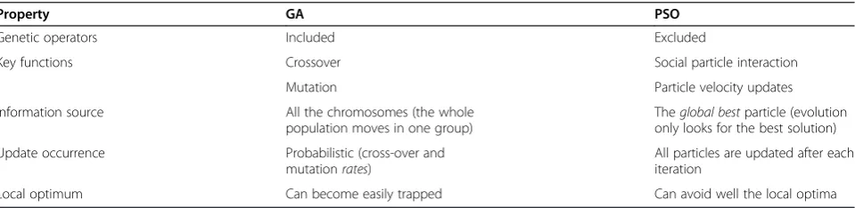
for audio feature selection and synthesis. The main mo-tivation for the work is to provide improved content-based audio classification and retrieval performance. To motivate the selection of PSO instead of the generally applied GA (or its derivatives), a comparison of the two algorithms, based on [9], is provided in Table 1. In short, the main advantage of PSO over GAs is that the algo-rithm provides more profound intelligent background [28], and it can be performed more easily than GAs [28]. Also, the computation time of PSO is usually less than for GAs, because all the particles in PSO tend to con-verge to the best solution rather quickly [29]. The syn-thesis approach presented in this article provides the ability to apply any fitness measure found appropriate for the final feature task at hand (such as classification). Furthermore, we apply amulti-dimensional extension of the basic PSO algorithm (MD PSO, [30]) to allow dy-namic output FV dimensions. This avoids the need of fixing the dimension of the solution space (correspond-ing to the dimensionality of the synthesized vector) in advance, which is a property not considered in the audio feature generation methods published before.
In order to better avoid the problem ofpremature con-vergence related to the traditional PSO, a recent tech-nique, the fractional global best formation (FGBF) suggested in [31], is also adopted within the proposed synthesis approach. A preliminary work was presented in [32], in which the performance improvement pro-vided by the approach was tentatively verified in the context of images. Furthermore, in this article, a hetero-geneous particle behavior approach, recently proposed by Engelbrecht [33], is considered. The approach pro-vides further assistance for the particle swarm to con-verge to the global optimum of the search space by altering the particle velocity update rules. Hence, finally, as a combination of all the PSO extensions, in this study we propose applying an MD PSO algorithm with FGBF and heterogeneous particle behaviors for audio feature synthesis. To the best of the authors’knowledge, we are not aware that such an approach (or PSO in general) should have been proposed earlier in the audio feature generation field.
Table 1 Comparison of GA and PSO as search algorithms
Property GA PSO
Genetic operators Included Excluded
Key functions Crossover Social particle interaction
Mutation Particle velocity updates
Information source All the chromosomes (the whole population moves in one group)
Theglobal bestparticle (evolution only looks for the best solution)
Update occurrence Probabilistic (cross-over and mutationrates)
All particles are updated after each iteration
The rest of the article is organized as follows. The low-level audio features considered in this research are described in“Low-level audio features”section, whereas in “Evolutionary optimization techniques” section, the underlying evolutionary optimization technique, the MD PSO, is introduced in detail.“EFS and selection”section presents an overview and technical details of the pro-posed feature synthesis approach, and the experimental results with comparative evaluations are shown and dis-cussed in “Experimental results” section. Finally, “ Con-clusion” section concludes the article and discusses topics for future research.
Low-level audio features
In order to provide some important background infor-mation for the ultimate goal of this study, i.e., improving the audio retrieval performance, we start by introducing the applied original (low-level) audio features and the extraction procedures preceding the actual feature syn-thesis process. As mentioned in “Introduction” section, audio features play an essential role in content-based classification and retrieval tasks, so that selecting and extracting the“correct”features for the problem at hand is of utmost importance. Thus, the major focus is on synthesizing new features from the low-level audio fea-tures most typically used in the literature. This provides us a solid “baseline” FSs and allows us to demonstrate the effectiveness of the proposed synthesis technique.
Two separate audio feature extraction approaches are used to evaluate the performance of the feature synthesis with different types of features. In order to detect specific temporal signal characteristics, the considered audio clips are processed in short time frames of 40-ms duration. The first approach extractssegment-basedfeatures, while the second one is based on the so-called “bag-of-frames” approach [34], where the features are extracted directly from the short-time frames. The details of the extraction methods are provided in the following sections.
Segment features
The segment features are extracted based on the method introduced in [35]. Theenergy levelsof the audio frames are computed, and then compared to the average energy level of the whole audio signal to detect and discard si-lent audio frames. In the second phase, seven audio FSs (specified on the left column of Table 2) are extracted from the non-silent frames, and consecutive non-silent frames are merged to form distinct audio segments. Hence, theoretically, an audio signal with no silent sec-tions would be considered as a single segment. However, due to some background noise or environmental acous-tics, occasional non-silent frames may occur in the mid-dle of a silent section. To filter out such noisy frames in the process, an empirically determined threshold of five
consecutive frames was set as a minimum duration for a signal segment. Finally, the actual audio segment fea-tures are formed by computing themean(μ) and stand-ard deviation(σ) statistics of eachFS (including also the STAT features, i.e., means of means, etc.) over the formed segments. Thus, as an example, an audio signal consisting of four separate segments is represented by four corresponding segment FVs of each FS. For a more detailed description of the segment feature extraction, the reader is referred to [35].
Key-frame features
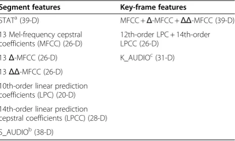
In the second feature extraction approach, the features are extracted directly from the short time frames. Due to this, the frames are first Hamming-windowed to avoid sharp discontinuities at the frame edges. Because there are many frames already in a single audio clip, a specific key-frame extraction method, proposed in [36], is ap-plied to reduce the mostredundantframes. Such redun-dancy occurs because many audio classes, such as music or speech, contain similar and almost identical sounds (such as common vowels or same notes of an instru-ment). In short, the main idea in the frame reduction ap-proach is to partition the extracted frame features into distinct clusters (based on their similarity/distance be-tween each other) and to select only one or few key -frames from each cluster to represent its corresponding sound. For this, aminimum spanning tree clustering al-gorithm is applied, which is detailed in [36]. As an out-come of the procedure, the overall amount of frames is Table 2 The extracted low-level audio features
Segment features Key-frame features
STATa(39-D) MFCC +Δ-MFCC +ΔΔ-MFCC (39-D)
13 Mel-frequency cepstral coefficients (MFCC) (26-D)
12th-order LPC + 14th-order LPCC (26-D)
13Δ-MFCC (26-D) K_AUDIOc(31-D)
13ΔΔ-MFCC (26-D)
10th-order linear prediction coefficients (LPC) (20-D)
14th-order linear prediction cepstral coefficients (LPCC) (28-D)
S_AUDIOb(38-D)
aSTAT includes the mean (μ) and standard deviation (σ) values of signal
statistical features, both in time and frequency domain: mean, variance, standard deviation, average deviation, skewness, kurtosis, andalsothe followingsegmentfeatures (μ,σ): band-energy ratio (BER), spectral centroid, transition rate, FF, irregularity (2 versions), flatness (both in linear and decibel scale), and tonality.
b
S_AUDIO includes the followingsegmentfeatures (μ,σ): tristimulus,
smoothness, spectral spread, spectral roll-off, RMS amplitude, inharmonicity, spectral crest, loudness, noisiness, power, odd-to-even ratio, and sub-band powers of six frequency bands.
c
significantly decreased, whereas most of the feature de-scription power is still maintained. The three frame-level FSs used in this study are listed on the right column of Table 2.
The extracted features of Table 2 represent an inclu-sive set of common audio features found from the litera-ture. The feature implementations are based on a publicly available“LibXtract”library [37], although some of the segment features, such as dominant BER and seg-ment FF, are extracted as described in [35]. The dimen-sions of the extracted FSs/vectors are also given in parenthesis for all sets in Table 2. For example, taking the mean and standard deviation of the 13th-order seg-ment MFCC features results to a 26-dimensional FV. The feature values of each segment/key-frame—as well as their corresponding ground truth class labels and clip indices (describing from which audio file a particular FV is extracted from)—are stored in a single plain text file, so that the actual audio files are not needed anymore after the feature extraction phase. For specific definitions and formulas for the extracted features, the reader is re-ferred to the audio signal processing literature (see, e.g., [38-40]).
Evolutionary optimization techniques
In this section, the PSO algorithm, its multi-dimensional extension, and the FGBF technique are introduced. The adaptation of heterogeneous particle behaviors within the MD PSO process is discussed in detail at the end of the section.
MD PSO
PSO was first introduced by Kennedy and Eberhart [7]. The PSO algorithm is a population-based optimization technique, in which a swarm of particles propagates in a pre-defined search space. Each individual particle, p, of the swarm represents a potential solution to an under-lying optimization problem, in which the particles are evaluated using a properfitness function,F½ p. The PSO algorithm is specifically designed for solving nonlinear optimization problems. Due to the diversity associated with randomly distributed particles, the algorithm is capable of searching the best solution among several local minima. After the initialization phase of the algo-rithm, where the particle randomization is performed, the particles are evaluated and moved iteratively in the search space. In order to eventually converge to the
global optimum of the search space, each particle p holds in its memory both social and cognitive terms, where the former corresponds to the best position found so far by the entire swarm (the global best) and the latter stands for the best position found by the particlepitself (personal best). As will be shortly seen, both the social and cognitive terms contribute in astochastic mannerto the particle position at the next iteration round.
An MD PSO algorithm was proposed in [30]. The al-gorithm allows the particles to make inter-dimensional jumps and visit any dimension, d, within a given range, d2½Dmin;Dmax. Thus, in order to provide improved fitness scores, the MD PSO searches for the global best solution among several search spaces with different dimensions. The particle navigation among the dimen-sions is controlled by a separate dimensional PSO process, which is interleaved with the regular positional update process. For this, each particle keeps also track of its personal (and the global) best dimension (from which the best fitness value so far has been achieved).
In a MD PSO process, the components of each par-ticlepat iteration roundtin a swarm ofP particles are presented as,
dpð Þt:dimensionof particlep,
xdpð Þt
p;j ð Þt :j th
element of thepositionof particlepin dimensiondp(t),
vdpð Þt
p;j ð Þt:j th
element of thevelocityof particlepin dimensiondp(t),
ydpð Þt
p;j ð Þt:j th
element of thepersonal best positionof particlepin dimensiondp(t),
vdpð Þt :dimensional velocityof particlep,
ydpð Þt :personal best dimensionof particlep,
^ yd
jð Þt :j th
element of theglobal best positionof the whole swarm in dimensiond, j,2[1,d]
^
ydðtÞ:global best dimensionof the whole swarm,
where (if not stated otherwise) j 2{1,. . .,dp(t)}. The
par-ticle fitness values are only evaluated within its current
di-mension, meaning that thepositionalPSO components in
all other dimensions remain the same for the next
iter-ation round t+ 1, that is, xd
pðtþ1Þ ¼xdpð Þt ; vdpðtþ1Þ ¼
vd
pð Þt ;ydpðtþ1Þ ¼ydpð Þt ;8d2½Dmin;Dmax∧d 6¼dpð Þt :
After computing the fitness score of each particle position
with the applied fitness function , the following update
equations are used for the personal best position and
ydppðtþ1Þðtþ1Þ ¼ y
dpðtþ1Þ
p ð Þt; if F xdppðtþ1Þðtþ1Þ
h i
>F ydppðtþ1Þð Þt
h i
xpdpðtþ1Þðtþ1Þ; else; ð1Þ
dimension of particlepfor iterationt+ 1: and
ydpðtþ1Þ ¼ ydpð Þt; if F x dpðtþ1Þ
p ðtþ1Þ
h i
>F yydpp ð Þtð Þt
h i
dpðtþ1Þ; else: (
ð2Þ
Furthermore, for each dimension d2½Dmin;Dmax, the global best particle position is updated as
^ydðtþ1Þ¼
(
^ydð Þt ;if min
p F y
d pðtþ1Þ
h i
≥F^ydð Þt
argmin
yd pðtþ1Þ
Fhydpðtþ1Þi
;else;
ð3Þ
and, finally, the global best dimension is updated as
^yd tð þ1Þ¼
(
^
y d tð Þ;if min
p F y
ydpðtþ1Þ
p ðtþ1Þ
h i
≥Fh^y^yd tð Þð Þt i
argmin ydpðtþ1Þ
Fhyydpp ðtþ1Þðtþ1Þi
;else;
ð4Þ
where, in both (3) and (4),p2½1;P.
The particle positions within the current dimension dp(t) are updated after each iteration as shown in (5), where w(t) is a so-called inertia weight, c1 and c2 are pre-determined constants,r1 andr2 are vectors of uni-formly distributed random variables, that is r1;j;r2;j
Uð0;1Þ;8j2 1;dpð Þt
, and∁z; Z
min;Zmax
½
ð Þworks as a
clamping operator that limits the elements of vector z between the specified values Zmin and Zmax. Typical PSO parameters [41] were used in this study, that is, the inertia weight was linearly decreased from 0.9 to 0.4, and c1 and c2 were both set to 2. The limiting values for the particle position, velocity, and dimen-sional velocity,X,V, andVD, respectively, were empiric-ally set into proper values, as will be discussed later in “Experimental results” section. Note that the new par-ticle position, xdpp ð Þtðtþ1Þ; remains in the current
di-mension dpð Þt after the positional update, whereas the
dimension may change afterwards in the dimension update process defined in (6), which is performed at the end of each iteration round. The b•c operator in (6) stands for a floor function, and r1 and r2 are now scalar uniformly distributed random variables; otherwise the update is performed similarly to the positional updates. For an interested reader, the pseudo-code and further details of the MD PSO are provided in [30].
vpdp;jð Þt ðtþ1Þ ¼w tð Þvdpp;jð Þt ð Þ þt c1r1;jð Þt ydpt
ð Þ
p;j ð Þt
xdpp;jð Þt ð Þt þc2r2;jð Þt ^ydpt
ð Þ
j ð Þ t x
dpð Þt p;j ð Þt
p;jdpð Þt
x ðtþ1Þ ¼xdpp;jð Þtð Þ þt ∁ v dpð Þt
p;j ðtþ1Þ;½Vmin;Vmax
xpdp;jð Þt ðtþ1Þ ∁ xdpp;jð Þtðtþ1Þ;½Xmin;Xmax
ð5Þ
vdpðtþ1Þ ¼ bvdpð Þ þt c1r1ð Þt ydpð Þ t dpð Þt
þc2r2ð Þðt ^yd tð Þ dpð ÞÞct
dpðtþ1Þ ¼dpð Þ þt ∁ vdpðtþ1Þ;½VDmin;VDmax
dpðtþ1Þ ∁ dpðtþ1Þ;½Dmin;Dmax
ð6Þ
FGBF algorithm
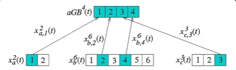
In some cases, the (MD) PSO algorithm suffers from the so-called premature convergence problem, meaning that the global best particle traps into a local minimum in the search space. This is especially true in high-dimensional and multi-modal search spaces, which are often encoun-tered in real-world applications. The problem is mainly caused by the loss of diversity, meaning that all the parti-cles are clamped too close to each other in the search space. A recent method called FGBF [31] has been pro-posed to tackle this problem by exploiting the potential of individual particleelementsof each particle position. The idea in the technique is to evaluate a separate fitness score for each particle element, in order to form an artifi-cial global best(aGB) particle by combining the best ele-ments found from the entire swarm. The formed aGB particle is then applied whenever it surpasses in fitness the regular global best particle, ^ydð Þt , of the swarm. For MD PSO, this means that a separate aGB particle needs to be assigned for each search space dimension, d2½Dmin;Dmax. However, in this case the aGB particle of a particular dimension can be also formed by combin-ing particle elements from dimensionsotherthan the cur-rent one. This is demonstrated in Figure 1, where elements from three different particles from separate dimensions,
xdpp;jð Þt ð Þt , are combined to form theaGBparticle. Such an approach increases the probability of finding an aGB par-ticle with a higher fitness score than the existing^ydð Þt so-lution for the dimensiondat stake. For the sake of clarity, pseudo-code for the FGBF approach within the MD PSO algorithm is shown in Algorithm 1.
Algorithm 1 Pseudo-code of the FGBF algorithm in MD PSO
Let½ ¼j arg minp2½1;PF x
dpð Þt p;j ð Þt
h i
, then
1. Select the best particle indices for each element,b[j], wherej2[1,Dmax], among all the particles,p2[1,P].
2. For (d2[Dmin,Dmax]) do:
a. Assign the best elements into theaGBsolution:
aGBd jð Þ ¼t x
db j½ ð Þt
b j½ ;j ;j2½1;d:
b. IfFaGBdð Þt <F^ydð Þt , then
^
ydð Þ ¼t aGBdð Þt :
3. Re-evaluate:^yd tð Þ ¼ arg mindF^ydð Þt :
Heterogeneous particle behaviors
As proposed recently by Engelbrecht [33], variation of the particlebehaviors, i.e., the velocity update rules, is another efficient way to enhance the convergence ability of the swarm in highly multi-modal problems. In addition to the particle velocity update equations (5) and (6), four other update models are introduced in this section. The models are extended to be used with the MD PSO approach so that the corresponding dimensional update rules are changed accordingly. Whenever a particle seems to get stuck into a local optimum, a new behavior model is assigned to it in a random manner. As well, the initial behaviors are chosen randomly for each particle.
Cognitive-only MD PSO model
In the cognitive-only MD PSO model [42], as the name suggests, thesocialterms^yjdpð Þtð Þt and^yd tð Þof the
parti-cles (i.e., the latter terms of (5) and (6) with thec2 coeffi-cients) are removed from the velocity update equations. This leads to broader particle exploration as interaction among particles ceases. This, instead, causes every par-ticle to become anindependenthill-climber in the search space. Thus, whenever the particle position is updated using this model, the (artificial) global best particle pos-ition is not considered in the update process.
Social-only MD PSO model
Like the previous model, in the social-only velocity rules [42], thecognitivetermsypdp;jð Þtð Þt andydpð Þt of the particles
(i.e., the former terms of (5) and (6) with the c1coefficients) are removed from the velocity update equations. Such a behavior provides faster particle exploitation, as now the entire swarm becomes a singlestochastichill-climber.
Barebones MD PSO
The Barebones PSO was suggested in [43], and in this model the velocity update rule is replaced by
vdpp;jð Þt ðtþ1Þ N y
dpð Þt p;j ð Þ þt ^y
dpð Þt
j ð Þt
2 ;σ
0 B @
1 C
A; ð7Þ
where σ ¼ ypdp;jð Þtð Þ t ^ydpð Þt
j ð Þt
: The position update
changes to xdpp;jð Þtðtþ1Þ ¼vdpp;jð Þtðtþ1Þ, so that the vel-ocity ends up being the new position of the particle, sampled from the described Gaussian distribution N . Similarly, for the particle dimensional velocity, the fol-lowing equation is applied
vdpðtþ1Þ N
ydpð Þ þt ^yd tð Þ
2 ;σ
; ð8Þ
where σ¼ydpð Þ t ^yd tð Þ. Again, the dimension
vel-ocity is considered as the actual new dimension, i.e., dpðtþ1Þ ¼vdpðtþ1Þ. Note that the clamping operation
is still applied to the obtained positions, so that the set limiting values are not exceeded.
In the positional point of view, the Barebones MD PSO facilitates aninitial exploration, because at first the personal best positions are far away from the global best solution, causing large deviations to the Gaussian distri-bution. However, as more iterations are performed, the deviation approaches to zero, causing the behavior to focus on exploitation of the average of the personal best and global best positions.
Modified barebones MD PSO
A modified version of the Barebones, also suggested in [43], is defined as
vdpp;jð Þt ðtþ1Þ ¼
ydpp;jð Þt ð Þt ; ifUð0;1Þ<0:5
N y
dpð Þt p;j ð Þ þt ^y
dpð Þt
j ð Þt
2 ;σ
0 B @
1 C A; else 8
> > > < > > > :
ð9Þ
and for dimensional update, similarly, as,
vdpðtþ1Þ ¼
ydpð Þt ; ifUð0;1Þ<0:5
N ydpð Þ þt 2 ^yd tð Þ;σ
; else: 8
< :
ð10Þ
regular Barebones), as now 50% of the time the focus is on the personal best solutions. As the process converges, the behavior will turn to exploitation, when all of the personal best solutions converge towards the global best solution.
As mentioned, each particle obtains its starting behav-ior randomly among the introduced models (including the regular one), after which the behavior is changed whenever a particle cannot improve its fitness score for the lasttenconsecutive iteration rounds. The whole idea here is that a new behavior model may help the particle to step out from a possible local optimum, and hence eventually provide improvements to the particle fitness score.
EFS and selection
As earlier discussed, the motivation behind proposing the EFS technique is to obtain enhanced audio features, so that audio classification and retrieval performance can be improved. In this section, we will describe the proposed feature selection and synthesis technique in detail. It will be shown that, with a proper encoding scheme (encapsulating several linear/nonlinear operators and the selected original features with their weights), the MD PSO particles can perform an evolutionary search towards finding the optimal synthesis parameters and output vector dimension. For this, a proper fitness meas-ure is to be designed, which maximizes the overall clas-sification (or retrieval) performance. The fitness functions applied in this study for evaluating the particle swarm performance during the synthesis procedure are introduced at the end of the section.
Definition of the main objectives
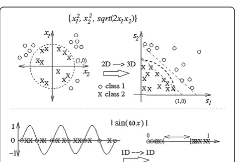
In an ideal case, a feature synthesis system, also called here as afeature synthesizer, receives as its input a spe-cific set of (low-level) audio features, selects the most representative and appropriate subset among them, combines and modifies the features by applying a proper set of transformation operators and feature weights, and finally produces a set of new and descriptive features in an optimal dimension with respect to the fitness func-tion assigned for the problem. Such an ideal feature syn-thesis operation (for the purpose of clustering) is demonstrated in Figure 2, where two-dimensional fea-tures of a 3-class dataset are successfully synthesized into clearly distinct clusters, enabling a much easier clas-sification and/or retrieval task compared to the original feature distribution. Note that, unlike in the figure, the proposed feature synthesis approach allows the output dimension to differ from the original dimension.
Changing the output dimensionality makes the ap-proach somewhat similar to SVM, which attempt to transform the original features into a higher dimension
to enable linear separation. However, a drawback with SVMs is their high dependency on the applied kernel function and the corresponding internal parameters, which may not fit to the problem at hand properly. This phenomenon is demonstrated in Figure 3, where two successful sample feature synthesizers are presented for a two-class classification problem. The upper case corre-sponds to an SVM with apolynomial kernel in a quad-ratic form. It is indeed capable of performing a proper transformation from 2D to 3D, enabling thus a linear separation between the two classes. However, in the lower case, a sinusoid with a proper angular frequency,
ω, needs to be applied instead for satisfactory class dis-crimination. Hence, it can be seen that searching for the correct transformation (instead of applying a fixed ker-nel) is of paramount importance, and this is actually considered as one of the main motivations for designing the feature synthesis scheme proposed in this article.
In light of the above discussion, the main objectives of the proposed EFS technique are to
perform a properfeature selectionamong the
original features,
Figure 3Two examples of feature synthesis (or transform) performed on 2D (upper case) and 1D (lower case) feature spaces using SVM.Depending on the original data distributions, different transformation functions are needed for successful feature separation.
search for the optimaloperatorsandfeature weights
for the synthesis process, and
search for the optimal output FV dimension among
a defined dimension range.
Overview of the proposed feature synthesis system To meet the aforementioned objectives, an evolutionary search procedure is performed. For each new synthe-sized feature (meaning a specific single feature in the generated output FV), the system, with a specified synthesis depthvalueK,
1. selectsK+ 1 original featuresf0,. . .,fK, ,
2 scales the selected features with proper weights
w0;. . .;wK ,
3. selectsKoperators,θ1;. . .;θK , to be applied over
the selected and scaled features, and
4. bounds the output with a nonlinear operator (here
tangent hyperbolicis applied).
Now, suppose that θnðfa;fbÞ, where n2½1;K, stands
for performing a specific operatorθnover the featuresfa and fb. Then, a formula for synthesizing a new feature sj can be defined as
sj¼tanh½θKðθK1ð. . .θ2ðθ1ðw0f0;w1f1Þ;w2f2Þ;. . .Þ;wKfKÞ;
ð11Þ
that is, first the operator θ1 is applied to the weighted features f0and f1, after which the operator θ2is applied to theresultof the first operation and the weighted fea-ture f2, and so on. Finally, the operator θK is applied to the result of all the previous operations and the weighted featurefK. With the details provided in“ Encod-ing of the particles” section, the dimension of the synthesized FV,s , along with the rest of the parameters in (11) are simultaneously optimized within the applied MD PSO search process.
In this article, the term “evolutionary” refers both to the underlying computing technique, the MD PSO, as well as to the nature of the feature synthesis process it-self, which can be performed in one or severalruns. The idea here is that each new run can further synthesize the features generated at the previous run and, hopefully,
further increase their discrimination power. A block diagram of the overall synthesis process is illustrated in Figure 4, where R synthesis runs are performed. The total number of runs,R, can either be determined in ad-vance oradaptively, in which case the fitness evaluation results are monitored after each run, and the process is stopped after no significant improvement is obtained anymore. Whether there should be more than a single set of features to be synthesized, an individual feature synthesizer will be evolved for eachFS. This is done in order to decrease the computational time needed for the overall processing, as this enables synthesizing the FSs in parallelby separate processes.
In a sense, the proposed EFS technique can be seen as a generalized form of artificial neural networks (ANN). Considering the four system steps listed above, a single-layer perceptron (SLP) classifier performs only steps 2 and 4, as neither feature nor operator selection is involved in the process. Instead, SLP does add a bias value to its weighted features, which can be mimicked also in our approach by inserting an additional constant value of 1 at the end of each original input FV (which the synthesizer can then select and scale among the other selected features). However, as no notable per-formance gain was witnessed by performing such an ac-tion, in the end the bias encoding is not considered in the proposed EFS technique. For further comparison, note that in the SLP topology the output layer dimen-sion is fixed, whereas in the EFS the output dimendimen-sion is (as mentioned) optimized within the set range. Also no-tice that performing several consecutive EFS runs corre-sponds to a multi-layer perceptron (MLP), or, in fact, any feed-forward ANN type. Similarly to SLP, the MLP does not include feature selection, and it also performs with fixed operator and output dimension. An important difference between the MLP and EFS approaches is that in the EFS technique the fitness of the synthesized FV is evaluated aftereach run, whereas in MLPs only thefinal fitness score in the output layer is considered, as the intermediate network layers are“hidden.”
Encoding of the particles
Recalling the PSO definitions introduced in “MD PSO” section, the position of a dp(t)-dimensional particlepat
time t, xdpp ð Þtð Þt , represents a potential solution on how
to perform the synthesis operation over the original fea-tures, that is, a potential synthesizer. The search space dimension, dpð Þt , corresponds to the number of features
synthesized into the output FV, that is, the output FV di-mension. Each particle position encapsulates a complete set of synthesis parameters: the indices of the selected features, the feature weights, and the selected feature operators. Accordingly, eachpositional elementof a par-ticle p, xdpp;jð Þt ð Þt , where j2 1;dpð Þt
, corresponds to a way of synthesizing the jth feature of the output FV. Thus, referring to the previously introduced four system steps, each such element must contain the following: K+ 1 indices for selecting the original features,K+ 1 fea-ture weights, and K operators in an encoded form to synthesize the corresponding output feature. For this, the positional elements of each particle in the particle swarm are encoded in avector formof length 2K+ 1, in-cluding K+ 1 “A-type” and K “B-type” components. These define the corresponding synthesis parameters as follows:
fn¼bAnc þ1;n2f0;Kg;
wn¼AnbAnc;n2f0;Kg;
θn¼dBne;n2f1;Kg;
ð12Þ
where the b•c and d•e operators correspond to the floor and ceiling mathematical integer functions, respectively. The value ranges for the components can be defined based on theinputFV dimension,F, and the total number
of operators available, Θ, as An2½0;F½andBn20;Θ.
The weight values are limited to 0≤wn<1.
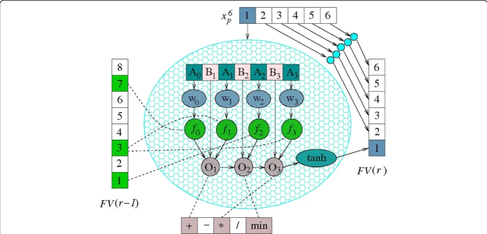
To give an example of the particle encoding scheme, Figure 5 presents a 6D particlepwith the corresponding synthesis process. Note that only the synthesis process of the first element of the output FV at run r, FV(r), is shown in detail, although a similar process is performed for all the output vector elements. For simplicity, the synthesis depth value, K, is set to 3, meaning that only K+ 1 = 4 features,f0,. . .,f3, are selected from input FV(r– 1). Thus, as demonstrated in the figure, each of the par-ticle elements includes 2K+ 1 = 7 encoded synthesis components, A0,. . .,A3 and B1,. . .,B3. The dimension of the input FV (which may either refer to the original FV consisting of a specific set of low-level features, or to an output FV from a previous EFS run, r – 1) is F= 8. As the total number of operators is set to Θ= 5, the value ranges for the two component types can be defined as An2½0;8 and½ Bn20;5. In Figure 5, the selected features
obtained by the underlying MD PSO process are the 7th, 3rd, 1st, and again the 3rd element of the input FV, while the corresponding operators are selected as ‘+’,‘min’, and ‘’Thus, performing the synthesis process as given in (11), the first element of the output FV is obtained by
s1¼ tanh min w0f½ 7 þw1f½ 3
;w2f½ 1
w3f½ 3
;
ð13Þ
wheref½ n stands for thenth element of the input FV.
Considering again the similarities of the EFS technique and an SLP classifier, it can be noticed that by setting
K+ 1 =F, discarding the feature selection as fn¼f½ n, and
setting each operator θn to ‘+’, the two approaches be-come identical. Similarly, by performing several runs with such synthesis parameters corresponds to an MLP approach with a one-to-one analogy between the num-ber of hidden layers and the numnum-ber of runs performed. In this sense, it can be stated that a regular feed-forward ANN is aspecial caseof the proposed EFS approach.
The fitness measures
Proper designing of the applied fitness measure plays an essential role in the feature synthesis process. The design is dependent on the intended use of the features, as the measured fitness value should highly relate to the object-ive of the synthesis process. Traditionally in content-based classification and retrieval scheme, specificsimilarity mea-sures, such as Euclidean distance, are applied to measure the distances between the FVs of a classified (or queried) item and each item belonging to the database. In a re-trieval case, the performance can be evaluated using the average precision (AP) metric, or the so-called average normalized modified retrieval rank (ANMMR), which is defined in the MPEG-7 standard [44].
As the main goal of the research is to improve audio retrieval performance by the means of feature synthesis, an intuitive approach for constructing a proper fitness function [] for the task would involve computing ei-ther the average retrieval precision (AP) or theANMMR values. However, neither option would be computation-ally feasible for large databases, as they both require conducting a separate batch query (i.e., selecting each item in the database as a query item one by one, per-forming a separate query for each of them, and finally taking the mean of the obtained retrieval results) for every fitness evaluation during the synthesis process. Therefore, in this article, we concentrate on obtaining a maximal discrimination between the features of differ-ent database classes, which should in turn result in improved retrieval performance. To achieve this we propose two alternative ways to form the fitness func-tion, described in the following sections.
Discrimination measure
First, a measure for evaluating the discrimination capabil-ity provided by the synthesized features is proposed. The measure is based on two widely used criteria in clustering:
Compactness: the database items of one cluster should be similar and close to each other in the feature space, and
Separation: different clusters and their centroids should be distinct and well separated from each other.
Suppose the different labels of anL-class database are denoted asl0;. . .;lL1, and the corresponding class cen-troids asμ0;. . .;μL1. Then, the followingdiscrimination
measure (DM) can be defined over a set of synthesized FVs,S= {s},
DM½ ¼S FPð Þ þS δmeanð Þln =δminðln;lmÞ;
where
δmeanð Þ ¼ln
1 L
XL1
n¼0 X
8s2lnkμnsk
ln
j j ;
δminðln;lmÞ ¼ minn6¼mðkμnμmkÞ:
ð14Þ
The terms of (14) are defined as follows: FP(S) stands for the number of false positive FVs occurring among the synthesized FVs S, meaning that those FVs are actu-ally located in closer proximity to some other class cen-troid than their own, δmeanð Þln is the average intra-class
distance, and δminðln;lmÞ corresponds to the minimum
centroid distance among all the classes. Thus, the dis-crimination measure, DM[S], strives for minimizing the intra-cluster distance, while maximizing the shortest inter-cluster distance. Ideally, each synthesized feature is in the closest proximity of its own class centroid, thus leading to a high discrimination among classes as illu-strated in Figure 2. However, minimizing the DM does not always lead to improved retrieval results. This is due to the fact that query items located at the outskirt of their own classes may be actually situated in closer prox-imity to some other FV located on the outskirt of its corresponding (wrong) class. Thus, in order to improve not only the feature discrimination in the feature space, but also the audio retrieval performance, next we propose applying a similar methodology that is utilized in feed-forward ANNs.
Target vector assignment
In the second approach, the idea is to assign a binary synthesizer target vector for each class, and let the underlying optimization algorithm to search for the proper synthesis parameters producing the desired out-put. The actual fitness value is then obtained by compar-ing the obtained and desired output vectors in a mean square error (MSE) sense. However, as the output di-mension of the EFS is not fixed in advance, a separate target vector is generated for each dimension d2
Dmin;Dmax
½ , resulting to a complete target matrix. For producing the matrix, a so-called error correcting output code[45] analogy is applied, which suggests two criteria for generating proper binary target matrices:
Column separation: Also the columns of the target matrix should be well separated from each other in the terms of Hamming distance.
Large row separation allows the synthesized vectors to differ somewhat from the actual target vectors with-out losing the discrimination between different classes. The reasoning for large column separation follows from the fact that each column in the target matrix can be seen as an individual binary classification task (between the classes having a value 1 and the classes having a value −1 in a specific column). Because of the varying similarity between two arbitrary audio classes, some of such binary classifications are likely to become much easier than others. Hence, as the same target vectors are nonetheless applied to any given in-put classes, it is also beneficial to keep the binary clas-sification tasks as different as possible by maximizing the column separation.
To generate a binary matrix with maximal row and column separation, the following matrix generation pro-cedure is used:
1. Compute the minimum number of bits,bmin, needed
to represent the total number of classes,L, in the database.
2. Form an empty matrix withLrows.
3. For each row, assign a binary representation of the row numbern2½0;L1as the first/nextbmin
target vector values.
4. Move the first row of the matrix to the bottom and shift the other rows up by one.
5. Repeat the steps 3 and 4 untilDmaxtarget vector
values have been assigned.
6. Replace the firstLvalues of each target vector with a 1-of-Lcoded [46] section.
The procedure generates new columns until the matrix is rotated back to its original order, resulting into a high column separation. Simultaneously, the row sep-aration is greatly increased compared to the regular 1-of-Lcoding section. However, in practice it was observed that for distinct classes it is often easiest to find a synthesizer that discriminates a certain single class from the others, and, therefore, sparing the 1-of-Lcoding sec-tion at the beginning of the matrix generally improves the synthesis results. For the vector dimensionsd<Dmax, only the firstdelements of the target vectors are consid-ered. This yields identical target vector elements be-tween the vectors of different length, allowing the FGBF algorithm to combine particle position elements from different dimensions (refer to FGBF algorithm).
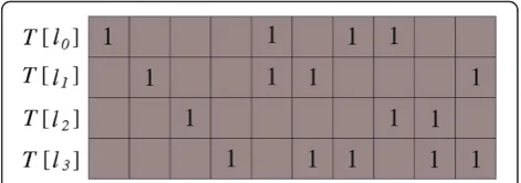
For clarification of the procedure, a target matrix for a 4-class database is demonstrated in Figure 6, where the
maximum dimension is set to Dmax= 10, and the mini-mum number of bits needed to represent the L= 4 classes is bmin= 2. The empty entries of the matrix cor-respond to values−1, andT l½ n stands for a target vector
for classln. As illustrated in this example, the generated matrix follows the provided algorithm with its 1-of-L coding section for the first L elements, followed by the elements created by the shifted rows of 2-bit row num-ber representations.
By applying the definitions given above, the fitness value for thejth elements of all the synthesized FVs, Sj, can be computed as
Fj Sj ¼
XL1
n¼0 X
8s2ln
T l½ njsj
2
; ð15Þ
whereT l½ njdenotes the jth element of the target vector
of class ln, and sj is the jth element of a single synthe-sized output vector belonging to classln. The overall fit-ness score F½ S can then be formed by adding the fractional fitness scores Fj Sj together and applying
normalization with respect to the number of dimensions. However, due to an observation that the first L vector elements, having the 1-of-L encoding, are usually the easiest ones to synthesize (and thus mainly favored in the dimension search by the MD PSO algorithm), the first L vector elements are handled separately in the summation process. Thus, for the dimensionsd>L, the normalizing divisor is strengthenedby an additional power parameter α> 1, which is to moderately increase the probability of converging into higher output vector dimensions whenever found beneficial. As a result, the overall fitness functionF½ S can be formulated as
F½ ¼S 1 L
XL
j¼1 XL1
n¼0 X
8s2ln
T l½ njsj
2
þ 1
dL
ð Þα
Xd
j¼Lþ1 XL1
n¼0 X
8s2ln
T l½ njsj
2
; ð16Þ
in which it is assumed thatDmin>L.
Experimental results
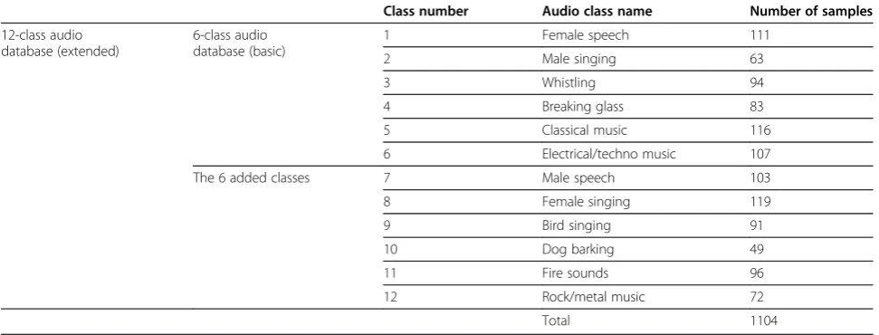
The EFS technique proposed in this article was tested with several audio classification and retrieval experi-ments using two separate audio databases. The first database consists of six distinct classes, while the second one was created by adding another six classes to the first database to form a more challenging 12-class database. The contents of the two databases are shown in Table 3, where the class numbers ranging from 1 to 6 belong to the basic database of 6 classes, and the extended data-base with 12 classes includes also the class numbers ran-ging from 7 to 12. The audio class samples are collected from a few different data sources; the speech classes (class nos. 1 and 7) are derived from the TIMITa data-base, the music classes (class nos. 5, 6, and 12) are from the RWC Music Databaseband another music collection at Tampere University of Technology (TUT), the “ gen-eral”audio sounds (class nos. 4, 9, 10, and 11) were pur-chased from the StockMusic.com webpage,c and, finally, the singing and whistling samples (class nos. 2, 3, and 8) are self-recorded and produced at TUT. The reasoning for two separate databases is to evaluate the scalability of the proposed feature synthesis system to more com-plex and difficult classification and retrieval tasks (i.e., to those cases where good features are truly needed).
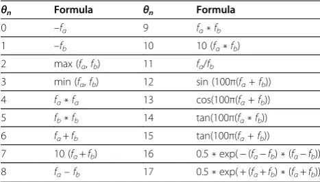
In the experiments shown in this section, unless stated otherwise, the following parameters and settings were used for the EFS: the depth of the synthesis was set to K= 7, meaning that 7 operators and K+ 1 = 8 features were chosen for the synthesis process of each output vector element, and the total number of operators, listed in Table 4 for featuresfaandfb, was set toΘ= 18. Simi-larly, the parameters for the MD PSO algorithm were set as follows: the swarm size was set to P =600 particles, 1,500 iterations were used, the dimension ranges for the basic and extended databases were set as ½Dmin;Dmax ¼
7;45
½ and ½Dmin;Dmax ¼½13;45, respectively, and the dimensional velocity range was experimentally deter-mined as ½VDmin;VDmax ¼ ½ 6;6 . Finally, the param-eterα> 1 used in (16) was determined separately for the key-frame and segment features as α=1.15 and α=1.3, respectively, as these values were found out to yield the best trade-off between the computational cost caused by higher dimensionality and the possible lack of perform-ance caused by reduction of the synthesized FV dimension.
In this study, separate “training sets” were considered for both databases. The training sets were formed by random selection, such that 45% of the audio clips of each class from both databases were included to them. Analogous to supervised machine learning, extracted features of these training sets were then used in search-ing the most suitable synthesis parameters for the corre-sponding databases, after which the found parameters were applied in synthesizing the features of the whole data. Thus, after the parameter search process, the resulting EFS system may synthesize new features for the rest of the (unseen) data without further optimization processes. The final obtained synthesized features were tested with multiple evaluations, demon-strating their enhanced discrimination capabilities over the original FSs.
Performance evaluations on feature discrimination We will first concentrate on evaluating the feature DM of the original and synthesized FSs. The DM was given in (14), and the obtained results for the original and synthesized segment- and key-frame-level audio features of low-level audio features are shown in Table 5. Recall that the higher the DM value, the more the features are mixed up with each other in the feature space (indicating less discrimination). As
Table 3 The contents of the two audio databases
Class number Audio class name Number of samples
12-class audio database (extended)
6-class audio database (basic)
1 Female speech 111
2 Male singing 63
3 Whistling 94
4 Breaking glass 83
5 Classical music 116
6 Electrical/techno music 107
The 6 added classes 7 Male speech 103
8 Female singing 119
9 Bird singing 91
10 Dog barking 49
11 Fire sounds 96
12 Rock/metal music 72
expected, it can be seen that discriminating the fea-tures of the extended 12-class database is significantly more challenging than those with the basic database. However, after performing the feature synthesis pro-cedure with the found synthesis parameters, substan-tial DM improvements were obtained for all the FSs. Note that, due to the stochastic nature of the under-lying optimization approach, ten separate EFS evalua-tions were performed for all the FSs, and the obtained mean (μ) and standard deviation (σ) values are also reported. The rest of the synthesis results presented in this section conform to the same protocol.
As the DM as such is not an intuitive measure of fitness for the FSs, we will concentrate on demon-strating the audio retrieval performances obtained with different FSs. Recall, however, that in general the usage of new synthesized features is not by any means restricted to merely retrieval purposes. Instead, as long as a proper fitness function can be designed, the EFS technique can be applied to basically any task requiring feature improvement. To show an example,
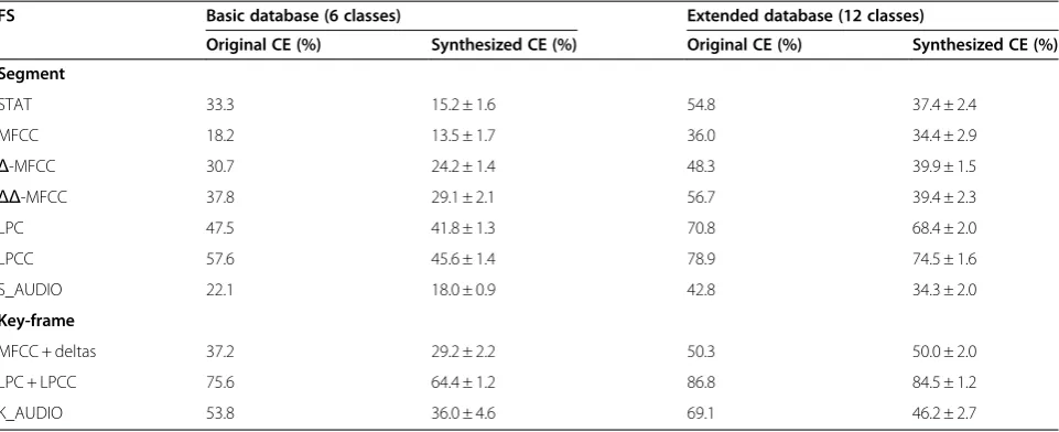
a rather obvious application is demonstrated, in which a K-means classifier is applied. The algorithm was first run with the formed training sets to compute the class centroids, after which the unseen (55%) test data samples were classified according to their closest class centroid. The classification error (CE) results obtained with the synthesized features for the both databases were compared to the errors associated with the original FSs. The results, shown in Table 6, indicate clearly improved classification performance obtained by the new synthesized features.
Performance evaluations on audio retrievals
For evaluating the audio retrieval performance, the metrics, ANMRR and AP, introduced in “The fitness measures” section were applied. In our approach, we first compute (using Euclidean distance) the distances between the first FV of a query item and all the FVs of a particular database item from which we take the mini-mum distance (normalized by the vector length) and store it. Second, we take the next FV of the query item and continue similarly with all the query item FVs. Fi-nally, before moving to the next database item, we take thesumof all the obtained minimum distances to obtain a single distance value between the queried item and the database item (which is used to rank that query item). In order to provide some baseline results, the ANMRR and AP values obtained by using a batch query and the ori-ginally extracted audio features are shown in Table 7. As expected, for both the segment- and the key-frame-based FSs, the retrieval performance deteriorates considerably as the database size increases from the basic 6-class database to the extended 12-class database. Like in the results shown in Tables 5 and 6, the segment MFCC features seem to provide the best performance among the original FSs.
Table 5 The DM statistics of ten separate EFS evaluations for the original and synthesized features
FS Basic database (6 classes) Extended database (12 classes)
Original DM Synthesized DM (μ±σ) Original DM Synthesized DM (μ±σ)
Segment
STAT 500.5 43.6 ± 6.7 1793 406.3 ± 47.6
MFCC 333.4 61.5 ± 8.5 1141 361.0 ± 22.4
Δ-MFCC 515.7 130.5 ± 7.9 1865 620.1 ± 27.1
ΔΔ-MFCC 622.6 140.9 ± 11.5 2072 532.7 ± 23.6
LPC 1114 270.3 ± 8.9 4520 1204 ± 29.1
LPCC 1638 310.3 ± 12.8 10830 1395 ± 26.5
S_AUDIO 342.6 56.0 ± 4.1 1365 382.8 ± 15.2
Key-frame
MFCC + deltas 2627 820.6 ± 53.6 7113 3093 ± 138
LPC + LPCC 6951 2143 ± 39.4 23 900 6378 ± 157
K_AUDIO 3150 782.7 ± 50.5 10 140 2774 ± 154
Table 4 The list of operators used in the feature synthesis process for featuresfaandfb
θn Formula θn Formula
0 –fα 9 fα*fb
1 –fb 10 10 (fα*fb)
2 max (fα,fb) 11 fα/fb
3 min (fα,fb) 12 sin (100π(fα+fb))
4 fα*fα 13 cos(100π(fα+fb))
5 fb*fb 14 tan(100π(fα*fb))
6 fα+fb 15 tan(100π(fα+fb))
7 10 (fα+fb) 16 0.5 * exp(−(fα−fb) * (fα−fb))
Next, a standard SLP classifier was trained with the MD PSO approach (by the methods described in [30]), in order to compare the proposed EFS technique with neural network-based approaches. Similar to EFS, an SLP can be treated as a feature synthesizer, in which case the original audio features are propagated through the network and the output layer dimensionality is set equal to the total number of classes, L. We call the resulting output vector a class vector, as it indicates the class designated for a particular input FV. The corresponding ANMRR and AP values obtained with these vectors are shown in Table 8. Compared to the values obtained with the original features, a clear improvement can be observed with nearly all the FSs, excluding some of the segment features of the extended database. As
mentioned in “Low-level audio features” section, this is most probably due to the fact that, because of the nature of the segment-based features, the total number of FVs per an audio clip is considerably less for segment fea-tures than for key-frame feafea-tures. Hence, because the FV dimensionality is highly decreased during the SLP synthesis process (to L), the extended database is ex-tremely complicated for an SLP classifier to learn with such a limited amount of data. In contrast, the basic database is well learned by the SLP, as an AP of nearly 90% is achieved with the segment-based MFCC features.
We will now demonstrate the significance of the add-itional properties associated with the EFS technique Table 6 CE of a K-means classifier over the original and synthesized features
FS Basic database (6 classes) Extended database (12 classes)
Original CE (%) Synthesized CE (%) Original CE (%) Synthesized CE (%)
Segment
STAT 33.3 15.2 ± 1.6 54.8 37.4 ± 2.4
MFCC 18.2 13.5 ± 1.7 36.0 34.4 ± 2.9
Δ-MFCC 30.7 24.2 ± 1.4 48.3 39.9 ± 1.5
ΔΔ-MFCC 37.8 29.1 ± 2.1 56.7 39.4 ± 2.3
LPC 47.5 41.8 ± 1.3 70.8 68.4 ± 2.0
LPCC 57.6 45.6 ± 1.4 78.9 74.5 ± 1.6
S_AUDIO 22.1 18.0 ± 0.9 42.8 34.3 ± 2.0
Key-frame
MFCC + deltas 37.2 29.2 ± 2.2 50.3 50.0 ± 2.0
LPC + LPCC 75.6 64.4 ± 1.2 86.8 84.5 ± 1.2
K_AUDIO 53.8 36.0 ± 4.6 69.1 46.2 ± 2.7
Table 7 The retrieval performances obtained with the original features for both audio databases
FS Basic database
(6 classes)
Extended database (12 classes)
ANMRR AP (%) ANMRR AP (%)
Segment
STAT 0.358 61.0 0.514 45.9
MFCC 0.228 73.8 0.367 60.2
Δ-MFCC 0.351 62.2 0.507 46.6
ΔΔ-MFCC 0.379 59.5 0.531 44.4
LPC 0.549 43.1 0.686 29.8
LPCC 0.569 41.1 0.717 26.9
S_AUDIO 0.263 71.0 0.450 52.3
Key-frame
MFCC + deltas 0.460 51.4 0.568 41.0
LPC + LPCC 0.637 34.8 0.787 20.4
K_AUDIO 0.375 59.5 0.524 44.9
Table 8 The retrieval performances obtained with the class vectors of an MD PSO-trained SLP classifier for both audio databases
FS Basic database
(6 classes)
Extended database (12 classes)
ANMRR AP (%) ANMRR AP (%)
Segment
STAT 0.238 75.0 0.626 36.4
MFCC 0.101 89.2 0.518 47.3
Δ-MFCC 0.339 64.7 0.581 40.0
ΔΔ-MFCC 0.290 70.1 0.585 40.1
LPC 0.491 49.7 0.673 31.3
LPCC 0.564 42.3 0.714 27.4
S_AUDIO 0.229 75.7 0.578 41.2
Key-frame
MFCC + deltas 0.279 70.2 0.414 56.5
LPC + LPCC 0.669 32.1 0.794 19.7
germane to SLPs. In the first demonstration, the feature selection property is enabled and applied to the input FVs, so that only K+ 1 = 8 original features are included into the actual synthesis process. The output FV dimen-sionality is fixed toL, and only the‘+’and ‘–‘operators are included in the synthesis process in order to mimic the behavior of typical neural networks (the subtraction operation is also needed to compensate with SLP weights, which are limited to [−1,1]). Such arrangements make the EFS similar to an SLP classifier (with the ex-ception of additional feature selectivity). The retrieval performance obtained with these settings is shown in Table 9, from where it can be seen that, excluding the MFCC features, the results are fairly comparable to those obtained with the SLP classifier. This is a result worth noting as onlyeight features were selected among the original input FVs. Such a reduction in the number of original features (without significant performance loss) suggests that at least some of them may not be es-sential to attain optimal discrimination capability.
In the next phase, the fixed output dimensionality of the synthesis method was changed so that the optimal dimensionality found using the underlying MD PSO al-gorithm was used in the synthesis process. All the opera-tors shown in Table 4 were included to the process to provide the synthesizer more possibilities for modifying the features. After the changes, a significant improve-ment in the retrieval performance was obtained, as shown in Table 10. Hence, optimizing the output FV dimension (and applying several operators in the synthesis process) significantly enhances the retrieval
performance. However, it should be noted that retrieval performance obtained with the original segment-based MFCC features of the extended database could not be improved either by the SLP classifiers or by the EFS experiments made so far. We believe this indicates that the MFCC features need to be treated as a whole and that selecting only few of them may decrease the overall retrieval performance. However, in this instance the per-formance drop is limited and clear perper-formance improvements relative to key-frame-based MFCC tures are still achieved. Also key-frame LPC + LPCC fea-tures show only minor improvements in AP values, which implies that certain audio features are not as synthesizable as others or that different types of arith-metic or logic operators may be required to achieve sig-nificant improvements in discrimination performance.
Finally, several consecutive EFS runs were performed to see whether the obtained synthesis results can be fur-ther improved (see Figure 4 in “Overview of the pro-posed feature synthesis system” section). Retrieval performance associated with certain synthesized FSs improved over several runs (<25), whereas some other features could not be enhanced notably. More generally, the segment-based features were more suitable for con-secutive EFS runs, as retrieval performance of the key-frame features remained rather stable during the runs. A graphical presentation of the experiments is shown in Figure 7, where the evolution of both the AP results and the synthesized FV dimensions over 25 synthesis runs are shown for several FSs and for both databases (L= 6/ L= 12). For simplicity, those FSs unable to demonstrate
Table 9 The retrieval performance statistics obtained using the EFS technique with fixed output dimension and only two operators
FS Basic database
(6 classes)
Extended database (12 classes)
ANMRR (μ±σ)
AP (%) (μ±σ)
ANMRR (μ±σ)
AP (%) (μ±σ)
Segment
STAT 0.278 ± 0.016 70.4 ± 1.7 0.534 ± 0.024 44.1 ± 2.4
MFCC 0.280 ± 0.022 69.6 ± 2.1 0.528 ± 0.023 44.9 ± 2.2 Δ-MFCC 0.375 ± 0.016 60.6 ± 1.6 0.574 ± 0.011 40.6 ± 1.0 ΔΔ-MFCC 0.393 ± 0.013 59.0 ± 1.3 0.598 ± 0.020 38.3 ± 2.0 LPC 0.549 ± 0.006 43.8 ± 0.6 0.729 ± 0.013 25.7 ± 1.2
LPCC 0.589 ± 0.015 39.6 ± 1.5 0.740 ± 0.006 24.8 ± 0.5
S_AUDIO 0.236 ± 0.015 74.7 ± 1.6 0.480 ± 0.013 49.9 ± 1.2
Key-frame
MFCC + deltas 0.463 ± 0.024 51.4 ± 2.3 0.629 ± 0.030 35.2 ± 2.8
LPC + LPCC 0.709 ± 0.007 28.4 ± 0.7 0.813 ± 0.003 18.0 ± 0.3
K_AUDIO 0.346 ± 0.016 63.0 ± 1.5 0.532 ± 0.012 44.4 ± 1.2
Table 10 The retrieval performance statistics obtained using the EFS technique with dynamic output dimension and 18 operators
FS Basic database
(6 classes)
Extended database (12 classes)
ANMRR (μ±σ)
AP (%) (μ±σ)
ANMRR (μ±σ)
AP (%) (μ±σ)
Segment
STAT 0.167 ± 0.013 81.7 ± 1.5 0.425 ± 0.012 55.0 ± 1.2
MFCC 0.221 ± 0.021 75.5 ± 2.2 0.398 ± 0.012 57.5 ± 1.2 Δ-MFCC 0.332 ± 0.015 64.7 ± 1.5 0.511 ± 0.096 43.9 ± 3.1 ΔΔ-MFCC 0.313 ± 0.016 66.7 ± 1.6 0.526 ± 0.033 45.0 ± 3.2 LPC 0.524 ± 0.016 46.1 ± 1.5 0.675 ± 0.008 31.1 ± 0.8
LPCC 0.556 ± 0.010 42.8 ± 1.0 0.720 ± 0.017 26.7 ± 1.6
S_AUDIO 0.171 ± 0.011 81.5 ± 1.2 0.442 ± 0.029 53.4 ± 2.9
Key-frame
MFCC + deltas 0.371 ± 0.012 60.3 ± 1.2 0.470 ± 0.012 50.5 ± 1.1
LPC + LPCC 0.634 ± 0.013 35.3 ± 1.2 0.775 ± 0.011 21.6 ± 1.0