R E S E A R C H
Open Access
Aerodynamic web forming: process
simulation and material properties
Simone Gramsch
1, Axel Klar
2, Günter Leugering
3, Nicole Marheineke
3*, Christian Nessler
2,
Christoph Strohmeyer
3and Raimund Wegener
1*Correspondence:
3Department Mathematik, FAU
Erlangen-Nürnberg, Cauerstr. 11, Erlangen, 91058, Germany Full list of author information is available at the end of the article
Abstract
In this paper we present a chain of mathematical models that enables the numerical simulation of the airlay process and the investigation of the resulting nonwoven material by means of virtual tensile strength tests. The models range from a highly turbulent dilute fiber suspension flow to stochastic surrogates for fiber lay-down and web formation and further to Cosserat networks with effective material laws. Crucial is the consistent mathematical mapping between the parameters of the process and the material. We illustrate the applicability of the model chain for an industrial scenario, regarding data from computer tomography and experiments. By this proof of concept we show the feasibility of future simulation-based process design and material optimization which are long-term objectives in the technical textile industry.
MSC: 65Mxx; 74Hxx; 74Kxx; 74Q15; 76T20
Keywords: airlay process; nonwoven material; virtual tensile strength test; fiber suspension flow; fiber lay-down; fiber networks; model chain; stochastic surrogates; homogenization; effective material laws
1 Introduction
Aerodynamic web forming addresses a broad spectrum of applications for the produced nonwoven materials. Airlay fabrics range from insulation and filter materials over automo-tive and mattress felts to medical and hygiene products depending on the type of entering fiber material (e.g., natural (cotton, flax, hemp, etc.), man-made fibers or even reclaimed textile waste). The fibers may have a length up to mm and a weight between and dtex ( dtex = –kg/m). In the airlay process the fibers leave from a rotating drum into a turbulent air flow. Suctioning onto a perforated moving conveyor belt leads to the forming of a random three-dimensional web structure, see Figure and []. The produc-tion of the final fabrics takes place in further post-processing steps. Simulaproduc-tion-based pro-cess design and management are a basis for the prediction and improvement of product properties and an objective in industry. This requires the mathematical modeling of the process which is topic of the paper.
The aerodynamic web forming is a multi-scale two-phase problem whose monolithic handling and direct simulation based on a model of first principles are not possible due to its high complexity. So far, no simulation results exist in literature. In this paper, we establish a consistent, accurate and efficiently evaluable chain of mathematical models
Figure 1 Industrial production of airlay fabrics.From left to right: Airlay machine (Airlay-K12 by machine manufacturer AUTEFA Solutions), aerodynamic web forming, nonwoven material.
towards the simulation of the airlay process and furthermore the investigation of the ma-terial behavior. The models cover the dilute fiber suspension with elastic slender bodies in the turbulent flow, stochastic surrogates for the fiber lay-down and web formation as well as Cosserat networks with effective material laws for tensile strength tests. They are coupled by means of parameter identification. We illustrate the applicability of the model chain for an industrial set-up, regarding computer tomography data and tensile strength experiments of the airlay nonwoven materials.
Table 1 Structure of the paper based on model chain
process simulation
fiber suspension flow dynamics and deposition
Section2
→
microstructure generation
stochastic fiber lay-down model elastic Cosserat network
Section3
→
material investigation
virtual tensile strength test effective material laws
Section4
Structure of the paper. The structure of the paper reflects the three relevant modeling steps concerning the fiber-loaded turbulent flow simulation (Section ), the microstruc-ture generation (Section ) and the effective material description and investigation (Sec-tion ), cf. Table . All models - apart from the surrogate fiber lay-down model - are orig-inated in the framework of fluid dynamics and solid mechanics, describing well-known conservation properties in form of (partial, ordinary, stochastic) differential equations. In spite of the similar background each model by itself is extensive and rich in variables and parameters. To handle the accompanying complexity in notation and to facilitate the readability of the paper, each section is organized in the same way: we present the single model, whereat numerical or algorithmic details are given in separate paragraphs. Em-bedding it into the model chain we explain its coupling with the other models and - as an example - we apply it to the industrial airlay process scenario that is specified in Section . as reference case. Ending with integrated simulation results from process to material we conclude with a discussion on the sensitivity of the parameters and an outlook to future optimization issues in Section .
1.1 Industrial airlay process, reference scenario
A typical airlay process with the rotating card cylinder, the aerodyamic web forming zone and the conveyor belt is sketched in Figure . For the process description we introduce a fixed Cartesian coordinate system{ex, ey, ez}inRwith respect to the machinery, whose origin is centered on the conveyor belt below the fibers’ dropping. We refer to the ma-chine direction (MD) ex and its cross direction (CD) ey, where the conveyor belt lies in the MD-CD plane (z= ). The associated MD and CD cut planes are given byy= const andx= const, respectively. Apart from boundary effects the process properties are homo-geneous in CD. In this paper we consider the industrial airlay plant K by the machine manufacturer AUTEFA Solutions (Figure ) with which the following reference scenario has been studied. As entering fiber material a mixture of % solid PES fibers and % bicomponent fibers whose core is made from PES and whose surface is made from PET at a ratio of : is considered. The mixing ratios refer to the mass. The fibers are homoge-neous with circular cross-sections, their properties are summarized in Table . The airlay machine is run with a mass ratem of . kg/s, the card cylinder rotates with an angular˙ speed vCof s–, and the conveyor belt with a width b of . m moves with a speed vBof . m/s. The produced nonwoven has a base weight W of . kg/mand a height H of . m. In post-processing the nonwoven material is reinforced by thermobonding where the bicomponent fibers have an adhesive effect. The tensile strength experiments are per-formed on the thermobonded nonwoven regarding DIN-norm (GME ). Note that all quantities are given in SI-units in this paper.
Figure 2 Airlay process.Left: Sketch of the process.Right: Illustration of the aerodynamic web forming zone with fiber-loaded flow in the considered K12-plant geometry (MD cut plane). Machine parts, i.e., rotating card cylinder, conveyor belt as well as baffle pipe and pressing roll, are displayed in grey, simulated single fibers are visualized in front of the air flow that is colored by the mean velocity magnitude, cf. Section 2.2.
Table 2 Fiber properties in reference scenario
Property Symbol Unit Bico fiber (PES/PET) Solid fiber (PES)
Line density, titer (ρA) kg/m 4.4·10–7 6.7·10–7
Density ρ kg/m3 1.325·10+3 1.38·10+3
Diameter D m 2.1·10–5 2.5·10–5
Length (straight | crimped) L| m 6.0|5.1·10–2 6.0|5.1·10–2
Crimp number C bow/m 7·10+2 5·10+2
Elasticity modulus E N/m2 3·10+9 3·10+9
Shear modulus G N/m2 1.035·10+9 1.035·10+9
Bending stiffness (EI) Nm2 2.6·10–11 5.6·10–11
Tensile strength S N/(kg/m) 3.3·10+5 3.0·10+5
a Roman font. Sets are denoted by caligraphic letters. We use a tensor calculus with the dot operator·and the tensor product⊗.
2 Process simulation
2.1 Elastic fiber dynamics in turbulent flows
Let⊂Rbe the flow domain with boundary∂,=∪∂. According to the Cosserat theory [] a slender fiber can be asymptotically represented by a time-dependent curve (e.g., its center-line) r :I×R+→with material parameters∈I= [,] and timet∈R+. Its dynamics due to inertia and bending, driven by turbulence can be described for fiber curve, velocity and tangential traction (r, v,N) by the following constrained partial differ-ential equations with multiplicative Gaussian space-time noise [, ]
∂tr= v, ∂sr= , (.a)
(ρA)∂tv=∂s
N∂sr–∂s
(EI)∂ssr
+ f(r, v,∂sr; u) + A(r, v,∂sr; u,k,)·∂stw, (.b)
supplemented with appropriate initial and boundary conditions, where (ρA) and (EI) denote the fiber line density (titer) and bending stiffness. The unknown traction N :
I×R+
→Ris the Lagrange multiplier to the pointwise inextensibility constraint in the Euclidean norm · (.a). The corresponding deterministic system is known as Kirch-hoff beam (or KirchKirch-hoff-Love equations), it results from the Cosserat rod model in the asymptotic limit when the slenderness parameter and the typical Mach number vanish []. Crucial for the dynamic fiber behavior are the aerodynamic drag forces that depend locally on the angle of attack (fiber tangent) and the relative velocity between fluid flow and fiber. Applying the stochastic force model by [], we presuppose an underlying statistic
k-turbulence description that provides the mean flow velocity u :×R+→R. Addi-tionally, it characterizes the turbulent flow fluctuations by the kinetic turbulent energyk
and the dissipation rate, i.e.,k,:×R+→R. The drag forces are composed of the mean f in a parametric dependence on the mean flow velocity u evaluated at (r,t) and of a fluctuating part. The fluctuations are particularly modeled as Gaussian space-time white noise with the vector-valued Wiener process (w :I×R+
→R) and the tensor-valued amplitude A that carries the correlation structure of the turbulence via a parametric de-pendence on the flow quantities u,kand. For details we refer to []. Arising contacts of the fiber with the geometry are realized by means of nonholonomic constraints. Let
⊂∂denote the domain boundary with walls. We introduce a signed distance function
h(·,t)∈C(R,R), satisfyingh= inandh> infor allt≥. Then, the momentum balance (.b) becomes
(ρA)∂tv=· · ·+λ ∇
h
∇h, (λ= ∧h> )∨(λ> ∧h= ) (.c)
with the associated Lagrange multiplierλ. Here,· · ·represents the whole of the right-hand side of (.b). For modeling a fiber’s deposition the contact approach can be combined with a Coulomb friction model (kinetic and dynamic), in whichλacts as normal force according to its physical significance.
Numerical treatment. Fiber-flow computations at industrial scale require a highly effi-cient numerical performance. We use the commercial CFD softwareaANSYS Fluent for the flow and the licensable research softwarebFIDYST for the fiber simulations.
over the control cells [si–/,si+/] are characterized with the indexi, yielding
dri= vidt, sri+/= ,
(ρA) dvi= s–(φi+/–φi–/) + fidt+ s–/Ai·dwt
with flux approximation
φi+/=Ni+/ sri+/– s
(EI) ssr
i+/.
The function values at si+/ =si+ s/ are indicated with the indexi+/. The occur-ring derivatives are approximated with first order finite difference stencils, for example,
sri+/= (ri+– ri)/ s. So, the discretized fiber becomes a polygon line with a fixed geo-metrical spacing for the spatial points associated with the nodes. The aerodynamic force terms are evaluated as fi= (fi–/+ fi+/)/ (analogously for Ai), this has the advantage that the tangents are only needed on the edges; fiber curve and velocity are averaged across the neighboring nodes. The necessary flow data is interpolated at the associated posi-tions. The stochastic differential algebraic system with time-dependent Wiener process wis temporally treated with an implicit Euler-Maruyama method. Although the aerody-namic forces fiin the core (in the fiber tangent and velocity) are implicitly incorporated, the flow data that appears in them is queried with the fiber position of the old time level, such that the resulting large nonlinear equation system can be solved using a Newton method with analytical Jacobi matrix and Armijo step-size control. The corresponding linear systems are treated with a band solver. The method is so well optimized with regard to assembling the Jacobian that the main effort per time step is due to the linear equation solver itself. For existence and convergence results we refer to [].
For the nonholonomic contact constraints a Lagrange parameterλiand a Boolean vari-ableδi∈ {, }are assigned algorithmically to each nodesi. The last characterizes the fiber movement type as either non-contacting (free) (δi= ) or contacting (δi= ),
(ρA) dvi=· · ·+δiλi ∇
hi
∇hi
dt and
λi= , ifδi= ,
hi= , ifδi= .
The equations are solved in dependence onδifor each time steptntotn+. Although the Lagrange multipliers are distributions, this creates no problems for a finite Euler step. If, at the end of the time step, the conditionh(ri,tn+) > for free nodes orλi> for contacting nodes is violated, the Boolean variable is switched to the other value and the entire time step is repeated for all nodes. This procedure is iterated until all fiber points move consis-tently. The required smoothness of the distance functionhis essential for the performance of the Newton method. In practice, geometries in CFD simulations are described as trian-gular meshes implyingh(·,t)∈C. It is smoothed via a linear combination of the triangle plane distance functions that are weighted by radial Gaussian kernels normalized to give a partition of unity. For a new smoothing procedure based on convolutions see [].
2.2 Aerodynamic web forming zone
the rotating card cylinder continuously over time according to the machine’s mass rate (Figure ). Due to their inertia they collide with the baffle pipe before they are suctioned onto the conveyor belt by the downwards directed turbulent air flow. The turbulent flow fluctuations cause the fibers to swirl and to form a random web. We are interested in the fibers’ distribution on the conveyor belt and their characteristic geometrical lay-down properties as starting point for generating the resulting nonwoven material by means of a stochastic surrogate lay-down model. Since the airlay process parameters are constant over time and all characteristic (statistic) properties are homogeneous in CD - apart from negligible boundary effects due to the plant edges - we can use the invariances when de-termining the transition probability of the process.
Consider the fixed Cartesian coordinate system{ex, ey, ez}of the machinery, whose ori-gin is located in the middle of the conveyor belt below the fiber dropping (cf. Section .). Letp:R→Rbe the transition probability that relates the fibers’ dropping distribution densityϕalong the card cylinder and their deposition distribution densityψ on the con-veyor belt over time, i.e.,
ψ(x,y,t) =
Rp(x,y,t;ˇy, ˇ
t)ϕ(yˇ,ˇt) dyˇdˇt.
Here, each fiber is represented by a single fiber point. Because of the process invariances in CD and time we have
p(x,y,t;yˇ,ˇt) =p(x,y–yˇ,t–tˇ; , ) =:p(x,y–yˇ,t–ˇt).
We assume a maximal throwing range and a maximal lay-down time, hence there exist
ymax> andtmax>tmin> such that
p(x,y,t) = for|y|>ymax,t∈/[tmin,tmax].
In the airlay process the fibers’ dropping is equally distributed along the card cylinder with release widthwand over the production timeT, i.e.,ϕ(y,t) = [–w/,w/](y)[,T](t)/(wT) in terms of characteristic functions. This yields a deposition distribution density that is inde-pendent ofyandtin the so-called region of homogeneityH. The existence of this region,
H=∅, is crucial for the production of a homogeneous nonwoven and can be ensured by adequate process settings. We get
ψ(x,y,t) =
wTg(x), g(x) = tmax
tmin ymax
–ymax p
x,y,tdydt (.a)
inH=
(y,t)y∈
–w +ymax,
w
–ymax ,t∈(tmax,T+tmin)
. (.b)
EspeciallyRg(x) dx= is satisfied. We refer tog as probability density function for the lay-down MD positions. In the simulation we obtain the transition probability directly from the computed deposition density when using a Dirac-distributed dropping,
Figure 3 Turbulent flow field in the airlay process.From left to right: Mean velocity magnitudeu, turbulent lengthlT=k3/2/and turbulent timetT=k/. The plant geometry is colored in grey.
Coming to the actual process simulation: in the proposed one-way coupling we perform a stationary two-dimensional computation of the unloaded flow (MD cut plane), where the conveyor belt is realized as porous medium using Darcy’s law. The flow quantities for the reference scenario are visualized in Figure . In addition to the mean velocity magnitude
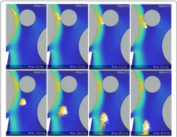
Figure 4 Typical fiber dynamics.Visualization of 100 bicomponent fibers (orange) and 100 solid fibers (white) that enter simultaneously the aerodynamic web forming zone and move over time. In the background the air flow is colored with the velocity magnitude, cf. Figure 3.
Figure 5 Fiber lay-down distribution.Probability distribution functionG(left) and densityg(right) of the lay-down MD position for the two fiber types (cf. (2.2a)),G(x) =–x∞g(x)dx. The MD position is given in the fixed coordinate system of the machinery, it indicates the distance to the card cylinder.
is approximated by the superposition of the point measures,gj(x)≈
n
k=δXjk(x)/nwith Dirac distributionδ, lay-down MD positionsXk
j associated to the fiber typej= , and
3 Virtual microstructure generation
The produced nonwoven consists of millions of fibers. We are interested in its material properties that are determined by the microstructure (Figure ). Since the described sim-ulations of single elastic fibers in the turbulent air flow are computationally expensive and very time-demanding due to the huge amount of physical details, we introduce a surrogate model for the efficient virtual three-dimensional web generation. We describe the ran-dom topology of the microstructure by help of a stochastic lay-down model in the spirit of [, ], whose parameters are calibrated using a representative process simulation (cf. Section .) and computer tomography data. On top of it we model the fiber associated material properties with an elastic Cosserat network. This network provides the basis for our virtual material investigations in Section . For modeling elastic multi-link structures we refer to [], see also [, , ].
3.1 Random fiber web topology
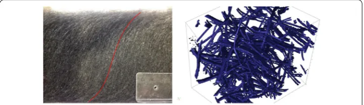
The nonwoven is the deposition image of the fibers. A striking characteristic in the mi-crostructure is a ramp-like contour surface, see Figure for a photo of a nonwoven sample. After the aerodynamic web forming the nonwoven material is thermobonded in a post-processing step. As result of heating the bicomponent fibers melt and glue the random individual fibers together to a solid fiber network which is then explored in material test-ing. Our strategy is to use the contour surface that results from the lay-down probability densities as basis for stochastic modeling the three-dimensional deposition image with crimped fibers. We identify the contact points of the fibers in the random web, specify the adhesive joints and generate the net topology by help of a graph where the adhesive joints are interpreted as nodes and the fibers as edges. The resulting network is equipped with constitutive relations in Section ..
We describe the contour line of the fiber material on the conveyor belt in MD by the graph ofR:R→[, H],
R(x) = H
x
–∞
rxdx, withr(x) =βn,g(x) +βn,g(x),βn,+βn,= , (.)
where H > denotes the height of the nonwoven andris the joined probability density of the deposited material,supp(r) = [xmin,xmax]. In particular,g andgare the MD lay-down density functions of the two different fiber types that are obtained from the process
simulation (cf. Figure and (.a)). The weightsβn,jcan be determined either with respect to the number ratio or the mass ratio of the fiber types. As we have a geometrical surrogate in mind, we use the number ratio that can be expressed by means of the known mass ratio
βm,/βm,, the fiber titers and lengths (Table ), so
βn,j=
βm,j(ρA)iLi
βm,(ρA)L+βm,(ρA)L, j=i,j= , .
Since the nonwoven is homogeneous in CD inH(.b), the contour lineRimplies a con-tour surface in the microstructure (Figure ).
Aiming for the three-dimensional nonwoven microstructure to investigate the material properties, we consider a cubic sample volumeV over the nonwoven height H with base areadthat is associated to the homogeneity regionH. As any fiber that can be partially contained inVlies inVR, i.e.,V= [–d/,d/]×[, H]⊂[–dR/,dR/]×[, H] =VRwith
dR=d+ L,L=maxjLj, we particularly deal with the reference sampleVR with the ex-tended base to avoid boundary effects. The microstructure is formed by the fibers’ falling onto the conveyor belt according to the contour surface (graph ofR) and the process mass ratem, while the belt moves with speed v˙ B. To account for the belt motion we introduce
xB: [,TR]→R,
xB(t) =xmin–
dR
+ vBt, TR=
vB(xmax–xmin+dR),
whereTRis the time needed to produce a nonwoven of the reference size. The total num-ber of finum-bers deposited uniformly in this time is given by
nj=βm,j ˙ m (ρA)jLj
dR bTR
for each typej= , with the mass associated weightsβm,j. The ratiodR/b with belt width b ensures the correct scaling in CD. Certainly, not all these fibers need to contribute to the reference sample VR because of the randomly distributed lay-down MD positions. In the following the index distinguishing the different fiber types is suppressed when not explicitly needed. We identify a deposited fiber with the lay-down timetand MD-CD-coordinates (X,Y) of its end point, i.e., (X,Y,t) withXbeinggj-distributed,Y uni-formly distributed in [–dR/,dR/] andt∈[,TR]. If especiallyX–xB(t)∈[–dR/,dR/] is satisfied, the deposited fiber contributes to the sampleVR. We model the fiber in the three-dimensional web as stochastic process in terms of the curve (e.g., its centerline)
η(X,Y,t):I→VR,
η(X,Ys ,t)= R(X)·ξs+X–xB(t)
ex+Yey+R(X)ez (.a)
with R(X) = +R(X)
I+ +R(X)– ey⊗ey+R(X)(ez⊗ex– ex⊗ez),
R(X)∈SO(), via the stochastic Stratonovich differential system []
dτs= –
B+
s(B)· ∇V(ξs) ds+As(√B)◦dws (.c)
withs(P) =ν1,s⊗ν,s+Pν,s⊗ν,s
withξ= ,τuniformly distributed in the unit circle spanned by exand eyas well as with Iunit tensor. By construction, a fiber end point lies on the contour surface and the main fiber orientation is aligned to it, since the tangential plane in the end point is spanned by ex+R(X)ezand ey. The underlying stochastic process ((ξ,τ) :I→R×S) with unit sphere S ⊂R in (.b)-(.c) is known as a three-dimensional anisotropic lay-down model for fiber position and orientation around the MD-CD plane, [, ]. It presents the path of a deposited fiber as image of an arc-length parameterized curve that is influ-enced by various (airlay) process parameters. Modeling the fiber orientation (tangent)τ, the drift term with the potentialVdescribes the typical coiling behavior of the fibers, i.e.,
V(ξ) =ξ·C–·ξ/ with C =diag(σ
x,σy,σz) regarding the machinery coordinates. In par-ticular,σx,σy≥ denote the standard deviations of the fiber throwing onto the conveyor belt in MD and CD, andσz> assures a height constraint. Accounting for the fluctua-tions in the airlay process, the drift is superposed by a white noise with the vector-valued Wiener process (w:I→R) and the scalar amplitudeA. The parameterB∈[, ] indi-cates the anisotropic behavior with the special local orthonormal right-handed director triad {τ,ν,ν}where ν∈span(ex, ey), i.e., isotropy forB= , asymptotic reduction to two-dimensional planar lay-down [, ] forB= .
On microscale the fibers are characterized by a crimp with crimp number C∈N(bows per unit length, cf. Table ). The crimp can be incorporated in the surrogate lay-down model by introducing a curveγ that describes the crimp structure and usingξ˜instead of
ξ in (.a), e.g.,
˜
ξs=
s
Qξ
s·dγ
ds
sds, γ(s) =sex+csin(Cπs)ey. (.)
The matrix-valued function Qξ : I → SO() represents the local ξ-associated triad {τ,ν,ν}with respect to the fixed coordinate system{ex, ey, ez}of the machinery. The parameterc≥ is implicitly given by the fiber length,
L =
ddγs(s)ds=
+c(Cπ)cos(Cπs) ds.
Superposing bicomponent and solid fibers according to their MD lay-down distribu-tions, number ratio and calibrated model parameters results in a virtual fiber web. To obtain the thermobonded nonwoven toVR, the adhesive joints in the web are detected by help of a contact thresholda≥ and the net topology is set up in terms of a graph. Details to the strategies and algorithms are given in the following subsections.
orientation is taken from computer tomography data (cf. Figure ). The respective image processing and analysis were performed and provided by the Fraunhofer ITWM, Depart-ment Image Processing with the softwarecMAVI.
Consider the discretized fiber data of a dynamical process simulation after deposi-tion on the MD-CD plane, i.e., dki = (rki,αki) with fixed cell size sand orientation an-gleαik∠(ex,∂srik),i= , . . . ,mfor each fiberk= , . . . ,ncorresponding to the same type, d= (dki). The noise amplitudeAis related to the change of orientation in the MD-CD plane. For endless fibers the throwing rangeσx,σyis given by the stationary deposition distribution, cf. ergodicity theorem in []. Using the sample of process simulations (Sec-tion .), we identify the parameters p = (A,σx,σy) as
p=f(d),
f(d) =
maxh∈N
n k= m–h i= (αk
i+h–αik)
n(m–h)h s,
n
k=
((rk– rk m)·ex)
n , n k=
((rk– rk m)·ey)
n
.
The finite length of the staple fibers might affect the result ifσ. In that case we estimate the parameters by the best approximation
p=argmin p∈(R+
)
fdsur(p)–f(d),
wheredsur(p) denotes the corresponding fiber data of the surrogate model (.b)-(.c). To solve the minimization problem, we apply a relaxated quasi Newton method with unit Jacobian and initial guess p =f(d) [].
Letθbe the angle of the fiber tangent out off the main plane. Its stationary distribution in the lay-down model (.b)-(.c) depends on the isotropy parameter B, i.e.,ρB(θ) =
cB(sinθ)/Bwith normalization constantcB. Using a data sampleθ= (θ, . . . ,θr) provided from a computer tomography scan of a material section, we determine Bby help of a maximum likelihood estimator
B=argmax B∈(,]
logf(B|θ), f(B|θ) = r
k=
cB(sinθk)/B.
The information aboutσzshould be also concluded from the computer tomography scan in future. However, so far, the image analysis yields no reasonable results, such that we approximate hereσz= .σy.
Figure shows the fiber deposition image associated to the reference scenario. The simulation of the stochastic lay-down model (.a)-(.c) is performed with an explicit Euler-Maruyama scheme with constant grid size s= –[s] and an underlying lay-down time resolution of t= –[m]. The calibrated model parameters are particularly p= (., .·–, .·–) for the bicomponent fibers and p
= (., .·–, .· –) for the solid fibers,B= .. The quantities are given in SI-units (A[m–/],σ [m],
Figure 7 Virtual deposition image.Virtual deposition image with contour surface according to MD lay-down distributions (3.1) and calibrated surrogate fiber models (3.2a)-(3.2c).Left and middle: The numbers of bicomponent fibers (blue) and solid fibers (red) are scaled down for visualization issues. Axes units in [10–2m].Right: Reference sampleVR.
Detection of adhesive joints. The microstructure of the thermobonded nonwoven is the random web of the deposited fibers that is glued together by the bicomponent fibers. In terms of graph theory the random net topology can be represented by a graphG= (N,E) where the adhesive joints are considered as the nodes and the fiber curves as the edges. Here,N andEdenote the index sets of nodes and edges, respectively.
For the identification of adhesive joints in the web (Figure , right), we restrict on the fiber points that are associated to the spatial discretization of the individual fibers (in the lay-down model) as possible contact points. With mpoints per fiberηandnfibers in total, comparing all data points with another has the complexityO((mn)). As we deal with plenty of fibers, a direct pointwise comparison would be by far computationally too expensive. The bounding box method that is well-known from computer graphics meets our demands on efficiency. For details and more sophisticated methods we refer to [, ] and references therein. We embed each fiber in a box aligned to the coordinate axes and check pairwise if the boxes intersect or not. If the intersection is empty, there are obviously no contact points. Otherwise, we restrict on the fiber parts in the intersection box and iterate the procedure. Finally, two cases can occur: either the intersection of the bounding boxes keeps unchanged or the number of fiber points in the intersection is sufficiently small. In both cases the naive pairwise computation of distances between the sets of fiber pointsFandFbelonging to two different fibers is used to detect possible contact points,
x,xˆ= argmin (x,ˆx)∈F×F
x–xˆ.
In general, this minimizer is not unique. We take the first minimizer found for practical reasons. Two fibers are considered to be in contact in the point a, if
x–xˆ≤a, a=
x+xˆ, (.)
where the contact thresholda≥ has to be chosen appropriately (see Section ). In case that a bicomponent fiber is involved in the contact, we refer to a as adhesive joint and replace xinFandxˆinFby a. The adhesive joints - together with the fibers’ end points
Figure 8 Fiber net topology.Net topology before (left) and after (right) contact detection for a section ofVR (cf. Figure 7, right),a= 10–5[m]. Disconnected fibers are deleted. Bicomponent fibers are colored in blue, solid
fibers in red. The adhesive joints are marked by the green circles, the fibers’ end points by the squares.
treating the set of all fiber discretization points as nodes. Disconnected subgraphs might be deleted from the network.
3.2 Elastic fiber net
For the subsequent material investigations we equip the fiber network with constitutive relations. An edge of the graphG= (N,E) is associated with a fiber piece. Due to its slender geometry angular momentum effects are negligibly small such that we model it as a truss. A truss network in a stress-free reference configuration is described by the set of fiber node points{rν∈R,ν∈N}and fiber edges r
μ∈P([,Lμ],R),drμ/ds= ,μ∈Ewhich are
related according to rνp∈ {r
μp(), rμp(Lμ)}for allμp∈E(νp). Here,E(ν) denotes the index set of edges connected to the nodeν, andPthe set of linear polynoms. The actual position rν, rμand inner forces nμof the truss network are determined by the system of differential
algebraic equations
drμ
ds = tμ,
dnμ
ds =α
rμ– rμ
, nμ=N(εμ)
tμ tμ
,εμ=tμ– , (.a)
μ∈E(ν)
nνμ= (.b)
for interior nodesν∈NI, supplemented with rν=rˆν(Dirichlet conditions) at fixed bound-ary nodesν∈NBd and nνμ= (stress-free conditions) at free moving boundary nodes ν∈NBs, whereN =NI∪NBd∪NBs. The force balance (.b) is fulfilled at all nodes with nν
μbeing the inner force of edgeμat nodeν. Along a fiber edge the truss model only admits
tangential forces. To incorporate the fiber crimp we use an effective elastic material lawN
for nμthat is nonlinear in the strainsεμand that we deduce from simulations of a
respec-tive beam model. Moreover, in contrast to a usual truss network model where dnμ/ds=
employ a Newton-Raphson method for the resulting system of nonlinear equations. Note that - alternatively to the position - the displacement field u = r – ris often considered as unknown in literature, see, e.g., [, ].
Effective force modeling based on beam behavior. We deduce the effective force modelN
for a truss (.a) from energetic investigations of stress-strain relations for a geometrically exact beam subjected to axial displacements. In the special Cosserat rod theory [] a beam is characterized by a curve (e.g., its centerline) r : [,L]→Rfor the position and a rotational group: [,L]→SO() for the orientation of the planar cross-sections. Let
{e, e, e}be a fixed outer orthonormal basis, then we consider a beam in the e-eplane. The quantities associated with a stress-free reference configuration are indicated with the index, in particular (r(L) – r()) =le,l≤L,0·e
= dr/ds= t(t= ) and0· e≡eare assumed. Hence, ris an arc-length parametrized curve of total lengthLwith
crimped lengthl. We model the beam deformations due to an axial displacementu∈Rin eby
dr ds = t,
d
ds =κ×,
dn ds = ,
dm ds = n×t,
n=·Cn·T·t– t, m=·Cm·T·κ–κ0
,
withr(), r(L)=r(), r(L) +ue,(s)·e= t/t(s),(s)·e= e,s∈ {,L}.
The material laws for inner forces n and torques m are linear in tangent t and curvature
κ, where Cn= (GA)PE/Gand Cm= (EI)PG/Ewith Pz=ze⊗e+ e⊗e+ e⊗e,z≥,
and the respective fiber properties E, G, A and I (cf. Table ). For numerical details to beam simulations we refer to [, ]. Evaluatingε=u/l,N= n(L)·efor variousu∈R,
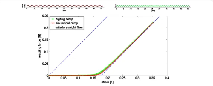
the resulting stress-strain relation of the beam model is exemplified for two variants of crimped fibers (sinusoidal and zigzag crimp) in Figure . The relation involves an effective elastic material lawN(ε),ε∈Rfor the truss model in (.a).
Since the stress-strain relation reveals two characteristic regimes we think of an analyt-ical surrogate that describes linearly fiber straightening for ≤ε<εand fiber stretching
forε>εwithε= (L–l)/l,
N(ε) =
N/εε, ≤ε≤ε,
N+ EA/( +ε)(ε–ε), ε<ε, N
= EI/lε
L
k(s)ds. (.)
In the straightening phase stretching is assumed to be negligibly small such thatNis
the force exclusively required to pull out the underlying crimp. In (.) k represents the geometrical curvature of the arc-length parametrized crimped initial curve r, i.e., (k)=dr/ds. The integralJ
k=
L
(k(s))dsdepends obviously on the crimp struc-ture, although the simulations indicate that the differences are small (cf. Figure ). Ana-lyzing the case of a sinusoidal crimp that has been proposed in (.), we proceed from the initial fiber curver˜(˜s) =˜se+csin(Cπ˜s)e,˜s∈[,l] with crimped lengthl, crimp num-ber C∈N (bows per unit length) and amplitudec≥. Note thatr˜ is not arc-length parametrized. Assumingδ=cCπto be small and performing an asymptotic expansion in
δyieldsJk= (Cπ)lε+O(δ). Hence,N≈(Cπ)EI holds. Changes in the crimp struc-ture might affect the real factor occurring in the force termN. For higher regularity the
surrogate effective force model (.) can certainly be smoothed inε. Moreover, the intro-duction of a barrier function for negative strains might be reasonable to prevent the truss (.a) from degenerating to zero length atε= –.
4 Investigation of effective nonwoven material behavior
The quality of the produced nonwoven material is assessed by certain properties, among others, the tensile strength. An experimental tensile strength test on thermobonded non-woven samples reveals the characteristic stress-strain relation for the material within the measurement accuracies (cf. Figure ). Being interested in numerical material investiga-tions we perform virtual tensile strength tests on basis of the microstructure generated in Section . For this purpose we further reduce the model complexity by applying ho-mogenization techniques and effective material laws in the spirit of [, ]. In the virtual strength tests we particularly study the influence of the model parameters.
4.1 Virtual tensile strength test
In the one-dimensional experimental tensile strength test a cuboidal material sample over the full fabric height H is glued with the upper and lower faces onto two parallel plates.
The plates are pulled apart in direction of the nonwoven height while the reacting tensile forceFis recorded as function of the strainε. The strain is thereby determined from the actual sample heightHasε= (H–H◦)/H◦with the referential heightH◦corresponding to a pre-tensioning forceF◦, see Figure .
The experimentally investigated sampleVEis in general too huge for direct numerical simulations, e.g., in the considered industrial scenario the total length of contained fibers is approximately km. Since the sample is taken from the homogeneity region of the air-lay process, it is plausible to assume that its stochastic behavior is in average periodic in the base directions (being associated to MD and CD of the process). Thus,VEcan be con-sidered as assembly ofndisjoint thin equal sample columns (cf. reference sampleVR, Sec-tion .), and its tensile behavior can be concluded from exclusively investigating a single columnVRand linearly superposing the result: the tensile force toVEequalsn-times the tensile force toVRfor given strain. To further reduce the model complexity for the virtual strength tests we approximate the column-like reference sampleVRwith the microstruc-ture generated in Section by an inhomogeneous truss model (see Figure ). Therefore, we determine an effective material law by means of energetic homogenization using the Hill-Mandel-principle [, ]. In an inhomogeneous truss model the inner (tangential) forceN: [, H]→Rarising from an applied tensile forcef obeys
d dsN
ε(s),s= , withN(H), H=f.
Considering a partition of [, H] into subintervalsIi= [si–,si),i= , . . . ,m, with respect to an increasing sequence of nodes{si}along the truss, (s,sm) = (, H), we imposeN(ε(s),s) =
Ni(ε(s)) fors∈Ii. Assuming dNi/dε= , the strains are constantε(s) =ifors∈Ii. Hence,
Ni(i) =f inIi, with|Ii|=hi,i= , . . . ,m (.)
holds according to the force balance. Regarding the sample columnVR, the truss intervals
Ii are identified with representative volume elements (RVE) of heighthithat reflect the contour surface of the microstructure and the effective force modelsNi are concluded from simulations of the elastic fiber net in the respective RVEs. In view of the tensile strength tests we restrict toNi:R+→R+, presupposingNi() = ,Ni()→ ∞as→ ∞ and surjectivity. By this, the existence of solutions to (.) is ensured. If several solutions are possible, we consider the smallest strain. Consequently, the effective tensile behavior of the underlying huge material sampleVEcan then efficiently be computed for given force
F∈R+
from the following effective strain and height functionsεef,Hef,
εef(F) = H
ef(F) –Hef(F◦)
Hef(F◦) (.)
withHef(F) = m
i=
hiεi
F
n ,εi(f) =min
argmin
∈R+
Ni() –f.
Figure 11 Reduction of sample complexity for virtual tensile strength tests.From left to right: sampleVE in experiment, column-like sampleVRof microstructure generation that is partitioned into a sequence of representative volume elements and approximated by an inhomogeneous truss model with effective material law.
Figure 12 Tensile strength simulation with RVE.RVE with fiber truss network forε= 0 (left) andε= 0.6 (right). Axes units in [10–3m]. Trusses
are colored with respect to inner forces: no forces in blue, increasing forces from dark/light green to deep red.
heighthi(Figure ), all fiber node points at the upper face are vertically shifted with mag-nitude u, i.e., rν= rν+uez, ν∈NB,up, while the ones at the lower face are kept at the
referential positions. At the lateral faces only motions on the face plane are allowed. Eval-uatingε=u/hi,Ni=
ν∈NB,up
μ∈E(ν)nνμ·ezfor variousu∈R+yields then the effective force function.
The partition and size of the RVEs are chosen with respect to two demands: the RVEs must show the characteristics of the microstructure (non-homogeneity over height, con-tour surface, fiber properties), while the computational effort for the simulation has to be practically manageable. In a RVE only connected subgraphs that contain fiber node points at both, the upper and the lower, faces contribute to the reacting force. Hence, without altering the tensile behavior, we delete all other components from the fiber net-work to reduce the degrees of freedom for the simulation. In addition free ends, i.e., nodes with multiplicity at which no boundary conditions are imposed, have no impact and are deleted. Serial subgraphs, where elements are connected by nodes with multiplicity at which no boundary conditions are imposed, might give rise to singularities in the numer-ics and may therefore be interpreted as a single edge with an adapted material law. For a visualization of a RVE under increasing tensile force we refer to Figure .
4.2 Stress-strain results
-Figure 13 Stress-strain results forVE.Results provided by measurements (black lines, cf. green region in Figure 10) and by simulations for varying model parameters: RVE heighthi[10–3m], net stiffnessα[N/m2] and contact thresholda[10–6m].
Here:hi= 10, 15 (blue, red lines);α= 10–6, 10–5.5, 10–5 (dashed, thick solid, thin solid lines);a= 7.5, 7, 6.5 (higheraimplies steeper slope of curves).
that are computed on basis of our established process model chain - match the experimen-tal ones in principle. But the simulation results are obviously affected by the model param-eters for the fiber net, as variations of the topological contact thresholda(.), material stiffnessα(.a)-(.b) and RVE heighthifor the vertical non-homogeneity (.) show, see Figure . As already discussed, the introduction of the parameterhiis due to numerical reasons. Its choice has to ensure the representative character of the RVE and can be de-termined by several simulation runs. In the industrial scenario at hand,hi≈.·–[m] yields reasonable results by trend. Investigating the impact of the other two parameters, the study of the contact threshold areveals a robust tensile behavior whereas changes of the net stiffnessα are very sensitive. A larger contact thresholdacauses an increas-ing number of adhesive joints and hence a more connected net topology. This implies a stiffer material behavior which is seen in slightly steeper stress-strain curves. However, this effect is mainly restricted to small strains, the further behavior (shape) of the curves is unchanged. In the airlay process the contact threshold of the net is related to the post-processing step of thermobonding. Depending on process parameters, such as adhesive properties of the used fiber material, temperature and duration of the thermobonding, the thresholdacould be calibrated from experimental data. In contrast toa, the link be-tween the model parameterαand the process parameters is not evident at all. From the mathematical point of viewαis a relaxation parameter that ensures the uniqueness of the truss network solution. It might be interpreted in the context of net stiffness due to fibers’ entanglement, but the explanation is vague. We observe that changingαstrongly affects not only the slope but also the curvature of the stress-strain curves. Note that in a classi-cal truss network modelα= holds true. At this point of the simulation study,α≈–. [N/m] turns out to give an effective material behavior of the specific nonwoven sample which is comparable to the measurements. However, to get a general understanding ofαin view of the airlay process parameters a sensitivity analysis in combination with a broader experimental study is necessary. At last, the simulated stress-strain curves indicate gen-erally a stiffer material behavior for higher strains than the measured curves. The reason might be that the net topology, in particular the adhesive joints, is kept in the simulation -even under large tensile forces, whereas the fiber web rips and undergoes plastic changes in the experiment. This discrepancy might be overcome by introducing an additional pa-rameter, a damage threshold, in the elastic net model. Its calibration requires certainly information about the nature of the adhesive joints and hence a deeper investigation of the post-processing step of thermobonding.
5 Conclusion and outlook
material properties by virtual tensile strength tests. For the long-term industrial objective, the simulation-based process design towards the prediction and improvement of product properties, the mathematical mapping between the parameters of process and material is essential. We gave a proof of concept and showed the feasibility of a future optimization by applying our model chain to an industrial set-up. Proceeding from an airlay process simulation with a highly turbulent dilute fiber suspension flow, we used the process pa-rameters (including fiber properties) and the numerically obtained deposition results to set up the stochastic surrogate model for the microstructure generation. Thereby, certain topological web parameters that characterize anisotropy, adhesive joints and height of the microstructure have to be identified from computer tomography data and calibrated by experiments (thermobonding effects). So far, the evaluation of the fiber distribution in height direction lacks from the image analysis of the computer tomography scans, but re-spective research work is in progress. The effective nonwoven material laws were deduced from the underlying fiber properties and simulation runs using energetic homogenization techniques. In the tensile strength tests the simulated and measured material behaviors match well for small strains but deviate for higher strains. This discrepancy might be due to plastic changes (rupture) that are not handled in the present elastic fiber net model. The break-up of adhesive joints could be certainly included but requires a deeper insight in the mechanism of thermobonding that was not analyzed in this paper.
At this point of research, however, we still face a difficulty: the model chain contains one parameter that was introduced for mathematical reasons, i.e., well-posedness of the elastic fiber net model, but turned out to strongly influence the tensile behavior. To gain understanding of its dependencies on the process parameters which will be necessary for future optimization issues, a sensitivity analysis in combination with a broader experi-mental study might be helpful.
Competing interests
The authors declare that they have no competing interests.
Authors’ contributions
The process simulation comes from SG, RW and NM, the microstructure generation from CN and AK, the material investigations from CS and GL. NM and RW established the consistent model chain from process to material. NM wrote and all authors approved the final manuscript.
Author details
1Fraunhofer ITWM, Fraunhofer Platz 1, Kaiserslautern, 67663, Germany.2Fachbereich Mathematik, TU Kaiserslautern,
Erwin-Schrödinger-Str. 48, Kaiserslautern, 67663, Germany. 3Department Mathematik, FAU Erlangen-Nürnberg,
Cauerstr. 11, Erlangen, 91058, Germany.
Authors’ information
The research work that is presented in this article was developed in a joint project with groups from the University of Nürnberg-Erlangen and Kaiserslautern as well as from the Fraunhofer Institute for Industrial Mathematics, Kaiserslautern. The project addressed mathematics for innovations in the technical textile industry. Two companies were involved in the project, supporting the work with data and experience. Selected as a EU-MATHS-IN success story, the results were presented at the ECMI Conference 2016.
Acknowledgements
The authors thank their industrial partners, Dr. Joachim Binnig and Christopher Schütt from AUTEFA Solutions as well as Olaf Döhring from IDEAL Automotive, for performing measurements, providing data and information about process and fabric and supporting the work with fruitful discussions. Moreover, the financial support of the German
Bundesministerium für Bildung und Forschung, Project OPAL 05M13, is acknowledged.
Endnotes
a www.ansys.com.
b www.itwm.fraunhofer.de. FIDYST is a software tool for fiber dynamics simulations, developed by the Fraunhofer
c www.mavi-3d.de. MAVI (Modular algorithms for volume images) is a Fraunhofer software for image processing,
analysis and visualization, for details we refer to [43, 44].
Received: 1 September 2016 Accepted: 18 November 2016 References
1. Albrecht W, Fuchs H, Kittelmann W, editors. Nonwoven fabrics: raw materials, manufacture, applications, characteristics, testing processes. New York: Wiley; 2006.
2. Wegener R, Marheineke N, Hietel D. Virtual production of filaments and fleece. In: Neunzert H, Prätzel-Wolters D, editors. Currents in industrial mathematics: from concepts to research to education. Berlin: Springer; 2015. p. 103-62. 3. Klar A, Marheineke N, Wegener R. Hierarchy of mathematical models for production processes of technical textiles.
Z Angew Math Mech. 2009;89:941-61.
4. Marheineke N, Wegener R. Fiber dynamics in turbulent flows: general modeling framework. SIAM J Appl Math. 2006;66(5):1703-26.
5. Marheineke N, Wegener R. Modeling and application of a stochastic drag for fiber dynamics in turbulent flows. Int J Multiph Flow. 2011;37:136-48.
6. Götz T, Klar A, Marheineke N, Wegener R. A stochastic model and associated Fokker-Planck equation for the fiber lay-down process in nonwoven production processes. SIAM J Appl Math. 2007;67(6):1704-17.
7. Klar A, Maringer J, Wegener R. A smooth 3D model for fiber lay-down in nonwoven production processes. Kinet Relat Models. 2012;5(1):57-112.
8. Doulbeault J, Klar A, Mouhot C, Schmeiser C. Exponential rate of convergence to equilibrium for a model describing fiber lay-down processes. Appl Math Res Express. 2013;2013:165-75.
9. Grothaus M, Klar A. Ergodicity and rate of convergence for a non-sectorial fiber lay-down process. SIAM J Math Anal. 2008;40(3):968-83.
10. Kolb M, Savov M, Wübker A. (Non-)ergodicity of a degenerate diffusion modeling the fiber lay down process. SIAM J Math Anal. 2013;45(1):1-13.
11. Grothaus M, Klar A, Maringer J, Stilgenbauer P, Wegener R. Application of a three-dimensional fiber lay-down model to non-woven production processes. J Math Ind 2014;4:4.
12. Briane M. Three models of nonperiodic fibrous materials obtained by homogenization. Modél Math Anal Numér. 1993;27(6):759-75.
13. Le Bris C. Some numerical approaches for weakly random homogenization. In: Kreiss G, Lötstedt P, Malqvist A, Neytcheva M, editors. Numerical mathematics and advanced applications 2009. Berlin: Springer; 2010. p. 29-45. 14. Lebée A, Sab K. Homogenization of a space frame as a thick plate: application of the bending-gradient theory to a
beam lattice. Comput Struct. 2013;127:88-101.
15. Sigmund O. Materials with prescribed constitutive parameters: an inverse homogenization problem. Int J Solids Struct. 1994;31(17):2313-29.
16. Raina A, Linder C. A homogenization approach for nonwoven materials based on fiber undulations and reorientation. J Mech Phys Solids. 2014;65:12-34.
17. Adanur S, Liao T. Fiber arrangement characteristics and their effects on nonwoven tensile behavior. Tex Res J. 1999;69(11):816-24.
18. Bais-Singh S, Goswami BC. Theoretical determination of the mechanical response of spun-bonded nonwovens. J Text Inst. 1995;186(2):271-88.
19. Farukh F, Demirci E, Sabuncuoglu B, Acar M, Pourdeyhimi B, Silberschmidt VV. Mechanical analysis of bi-component-fibre nonwovens: finite-element strategy. Composites, Part B, Eng. 2015;68:327-35.
20. Glowinski R, Pan TW, Hesla TI, Joseph DD, Périaux J. A fictitious domain approach to the direct numerical simulation of incompressible viscous flow past moving rigid bodies: application to particulate flow. J Comput Phys. 2001;169:363-426.
21. Hämäläinen J, Lindström SB, Hämäläinen T, Niskanen H. Papermaking fibre-suspension flow simulations at multiple scales. J Eng Math. 2011;71(1):55-79.
22. Hu HH, Patanker NA, Zhu MY. Direct numerical simulation of fluid-solid systems using arbitrary Lagrangian-Eulerian technique. J Comput Phys. 2001;169:427-62.
23. Peskin CS. The immersed boundary method. Acta Numer. 2002;11:479-517.
24. Stockie JM, Green SI. Simulating the motion of flexible pulp fibres using the immersed boundary method. J Comput Phys. 1998;147(1):147-65.
25. Svenning E, Mark A, Edelvik F, Glatt E, Rief S, Wiegmann A, Martinsson L, Lai R, Fredlund M, Nyman U. Multiphase simulation of fiber suspension flows using immersed boundary methods. Nord Pulp Pap Res J. 2012;27(2):184-91. 26. Tornberg AK, Shelle MJ. Simulating the dynamics and interactions of flexible fibers in Stokes flow. J Comput Phys.
2004;196:8-40.
27. Barrett JW, Knezevic DJ, Süli E. Kinetic models of dilute polymers: analysis, approximation and computation. Prague: Ne´cas Center for Mathematical Modeling; 2009.
28. Gidaspow D. Multiphase flow and fluidization: continuum and kinetic theory descriptions. San Diego: Academic Press; 1994.
29. Antman SS. Nonlinear problems of elasticity. New York: Springer; 2006.
30. Baus F, Klar A, Marheineke N, Wegener R. Low-Mach-number - slenderness limit for elastic rods. 2015. arXiv:1507.03432.
31. Lindner F, Marheineke N, Stroot H, Vibe A, Wegener R. Stochastic dynamics for inextensible fibers in a spatially semi-discrete setting. Stoch Dyn. 2016. doi:10.1142/S0219437175001622016.
32. Schmeisser A, Wegener R, Hietel D, Hagen H. Smooth convolution-based distance functions. Graph Models. 2015;82:67-76.
33. Scott DW. Multivariate density estimation: theory, practice and visualization. New York: Wiley; 1992.
35. Lagnese J, Leugering G, Schmidt E. Modeling, analysis and control of dynamic elastic multi-link structures. Boston: Springer; 1994.
36. Hohe J, Becker W. Determination of the elasticity tensor of non-orthotropic celluar sandwich cores. Tech Mech. 1999;19(4):259-68.
37. Munoz Romero J. Finite-element analysis of flexible mechanisms using the master-slave approach with emphasis on the modelling of joints [PhD thesis]. London: Imperial College; 2004.
38. Bonilla LL, Götz T, Klar A, Marheineke N, Wegener R. Hydrodynamic limit for the Fokker-Planck equation describing fiber lay-down models. SIAM J Appl Math. 2007;68(3):648-65.
39. Chang C, Gorissen B, Melchior S. Fast oriented bounding box optimization on the rotation groupSO(3,R). ACM Trans Graph. 2011;30(5):122.
40. Ericson E. Real-time collision detection. London: CRC Press; 2004.
41. Simo JC. A finite strain beam formulation. The three-dimensional dynamic problem - part I. Comput Methods Appl Mech Eng. 1985;49:55-70.
42. Hill R. Elastic properties of reinforced solids: some theoretical principles. J Mech Phys Solids. 1963;11(5):357-72. 43. Ohser J, Schladitz K. 3D images of materials structures - processing and analysis. Weinheim: Wiley-VCH; 2009. 44. Redenbach C, Rack A, Schladitz K, Wirjadi O, Godehardt M. Beyond imaging: on the quantitative analysis of


![Figure 10 Tensile strength test for thermobonded nonwoven material samples. Left[m],: Experimentalset-up (test DIN-norm GME 60349)](https://thumb-us.123doks.com/thumbv2/123dok_us/9610526.1943323/17.595.120.478.561.669/figure-tensile-strength-thermobonded-nonwoven-material-samples-experimentalset.webp)

