https://doi.org/10.5194/ars-17-177-2019
© Author(s) 2019. This work is distributed under the Creative Commons Attribution 4.0 License.
Singularity Expansion Method for thin wires and
the Method of Modal Parameters
Sergey V. Tkachenko1, Juergen B. Nitsch1, Felix Middelstaedt1, Ronald Rambousky2, Martin Schaarschmidt2, and Ralf Vick1
1Faculty of Electrical Engineering and Information Technology, Otto-von-Guericke University, 39106 Magdeburg, Germany 2Wehrwissenschaftliche Institut für Schutztechnologien – ABC-Schutz (WIS), 29633 Münster, Germany
Correspondence:Sergey V. Tkachenko ([email protected])
Received: 19 February 2019 – Revised: 25 June 2019 – Accepted: 19 July 2019 – Published: 19 September 2019
Abstract. Here, we describe a technique to define the Sin-gularity Expansion Method (SEM) poles for short-circuited thin-wire structures developed using the Method of Modal Parameters (MoMP). The MoMP method consists of in the expansion of the system of mixed-potential integral equa-tions (MPIE) into the Fourier series, including the kernels containing Green’s function. Corresponding equations for Fourier modes contain infinite matrices of p.u.l. inductance and capacitance, and the solution for current can be obtained using the infinity matrix of p.u.l. impedance. The SEM poles are given by the zeros of the determinant of this matrix. For the case of the symmetrical circular loop, this equation trans-forms to one well-know from the literature. Numerical inves-tigation of solutions for the poles of the first layer has shown good agreement with previously obtained analytical and nu-merical results for different wire configurations.
1 Introduction
Thin-wire transmission lines play an important role in EMC. Thin-wire transmission lines facilitate the transmission of the desired signals between electronic devices of different kinds. On the other hand, they are subject to different kinds of elec-tronic interferences. Induced voltages are often the cause of the failure of electronic devices. Different numerical meth-ods (e.g., MoM, FDTD) can be applied to calculate induced currents and voltages, but these are not very helpful for gain-ing insight into the physics of couplgain-ing phenomena (e.g., to make a qualitative analysis of the system response for various values of system parameters, including the case of a statisti-cally defined system or field parameters).
In contrast, the Singularity Expansion Method (SEM) (see pioneer paper Baum, 1971, and reviews of results in books Baum et al., 2012; Tesche et al., 1997) represents the scatter-ing object as a set of oscillators, in which complex frequen-cies are poles of the response function, which do not depend on the type of excitation of the system. This set of poles yield the main contribution to the coupling response of the object, both in the frequency and time domains. It also defines the radiation of the system and the scattering amplitude. More-over, the SEM poles can be used for the identification of the systems. Recently, this method has attracted increasing in-terest in connection to the problem of target identification (Myers et al., 2011a, b; Giri and Tesche, 2012). However, the main method for obtaining the SEM expansion for a general system is the processing of numerical (e.g., Method of Mo-ments) data (Senior and Pond, 1981; Singaraju et al., 1976).
technique can be applied for thin wires of arbitrary geomet-rical form and arbitrary excitations.
The rest of the paper is organized in the following. In Sect. 2, the method of modal parameters will be briefly de-scribed. In Sect. 3, we present the analytical approach and a numerical algorithm for finding the SEM poles. In Sect. 4, some numerical results and comparisons with other methods will be described. Section 5 concludes the paper.
2 Method of Modal Parameters for finite wires
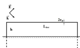
We consider a wire of arbitrary geometrical form above a perfect-conducting ground (Fig. 1). The wire is represented by a three-dimensional space curver(l)parameterized with its natural parameterl(0≤l≤L/2, whereL/2 is the length of the wire). It is assumed that both terminals of the line are connected with the ground. The wire is thin, i.e. the radius of the wire is essentially smaller relative to all other character-istic dimensions of the problem (e.g., wavelength λ, length of the lineL/2). The line is excited by an arbitrary electro-magnetic field, which can be external (e.g., an exciting plane wave) or a lumped voltage source (a load also can be consider as a current controlled voltage source). Since the thin-wire approximation is used, it is assumed that: the azimuthal com-ponent of the current is neglected; the charge density and the current are concentrated on the wire axis; and the boundary condition for the tangential component of the electric field is satisfied on the surface of the wire. The currentI (l0)and po-tentialφ (l)along the wire are described by the integrodiffer-ential Mixed Potintegrodiffer-ential Integral Equations (MPIE, e.g., Nitsch and Tkachenko, 2007). Usually, the system of MPIE is de-fined on the “physical” wire in the upper half-plane when the perfectly conducting ground is taking into account by mirror-ing the correspondmirror-ing Green’s functions. Another way is to add to a physical wire its mirror reflection and to consider the loop closed and completed (Fig. 2). During this procedure, the ground plane is removed. To excite only those modes, as in the initial problem, one has to also to consider a symmet-rical external and lumped excitation. Such a procedure yields the MPIE system for the closed loop:
dφ (l) dl +j ω
µ0
4π H
{L}
el(l)·el(l0)g(l, l0) I (l0)dl0=Eexl (l) H
{L}
g(l, l0)dI (l0)
dl0 dl0+j ω4π ε0φ (l)=0
; (1a)
el(l):=∂r(l)/∂l, |el(l)| =1; (1b)
g(l, l0)= e −j k
q
(r(l)−r(l0))2+r2 0
q
(r(l)−r(l0))2+r2 0
(1c)
HereL is the length of the complete wire loop,Elex(l)is a tangential component of a symmetrized exciting field,el(l)
is a tangential unit vector, andg(l, l0)is a scalar Green’s func-tion defined on the curved wire.
Figure 1.Inhomogeneous thin conductor over a conductive ground excited by external field and lumped source.
Figure 2.Short-circuited, semi-circular wire.
All functions of the natural parameterlin Eqs. (1a)–(1c) are periodical, i.e.,r(l+L)=r(l)and they can be expanded in a complete orthogonal set of functions exp(−j kml) with
km:=2π mL , m=. . .−1,0,1. . .They can be represented in
the form
Elex(l)= ∞ X
m=−∞
El,mex e−j kml= [e−j kml]T·Eex
l ; (2a)
φ (l)= ∞ X
m=−∞
φme−j kml= [e−j kml]T ·8; (2b)
I (l)= ∞ X
m=−∞
Ime−j kml= [e−j kml]T ·I (2c)
HereEexl ,8andI are column vectors of the Fourier coef-ficients of the exciting electric field, potential, and current; and[e−j kml] := [. . .e−j k−1l,1, ej k1l, . . .]T is an infinite col-umn vector of basic orthogonal functions.
−
jk·8+j ωL0·I=Eexl
−jk·I+j ωC0·8=0 ; (3a)
k=diag(km); (3b)
L0=µ0
2πGL; (3c)
C0= µ0
2π2π ε0G −1
C (3d)
where we introduce infinite square matrixes of inductance per-unit-lengthL0and capacitance per-unit-lengthC0, which can be obtained by expansion of the kernels of the sys-tem (Eq. 1a) in a double Fourier series:
GL= [GLm1,m2];
GLm1,m2= I
{L} dl1
I
{L}
dl2el(l1)·el(l2)g(l1, l2)
·exp(−j km2l2+j km1l1) (4)
GC= [GCm1,m2];
GCm1,m2= I
{L} dl1
I
{L}
dl2g(l1, l2)exp(−j km2l2+j km1l1) (5)
Using the modal representation of MPIE (Eq. 3a) one can easily obtain a formal solution for the column-vectors of the current and potential (Eq. 6), whereZ0 is an infinite modal impedance per-unit-length matrix (Eq. 7a), which defines the scattering field on
(
I=Z−1·Eex
l
8= 1
j ωC
−1·jk·Z−1·Eex
l
; (6)
Z0(j ω): =k·C 0−1·
k
j ω +j ωL 0
= η0
4π j k h
k·GC·k−k2GL
i
; (7a)
Escl = −Z0·I; (7b)
W =L
4Re
I+·Z·I ; (7c)
the boundary of the wire (Eq. 7b) and the radiation of the system (Eq. 7c) (Nitsch and Tkachenko, 2007).
The general solution (Eq. 6) is valid for any exciting field, including a plane wave excitation (Krauthauser et al., 2005) or lumped voltage sources (Nitsch and Tkachenko, 2005, 2007; Tkachenko et al., 2011). Moreover, lumped loads can be considered using current-controlled sources with un-known current amplitudes, which can be defined by solution of system of linear equations.
In this paper, however, we restrict our scope to the case of a short-circuited wire with an arbitrary excitation.
For the case of the semi-circular wire (when the closed wire is a circular loop, a structure with high symmetry with
constant curvature K=1/R=const and zero torsion T =
0), the modal inductance, capacitance and impedance per-unit-length are diagonal matrices and one can obtain a known solution for the induced current in the thin-wire approxima-tion (Wu, 1962)
L0m1,m2=L0m1δm1,m2; (8a)
L0m=µ0Rgm+1+gm−1
4 ; (8b)
Cm1,m2=Cm1·δm1,m2; (8c)
Cm=
2ε0 Rgm
(8d)
Zm1,m20 (j ω)=Z0m1(j ω)·δm1,m2; (9a)
Zm0 (j ω)=j ω Lm+
km2 j ω Cm
; (9b)
km:=
m
R, m=. . .−1,0,1. . . (9c) where
gm=
2π R
Z
0
ej kml−j k √
4R2sin2(l/2R)+a2
q
4R2sin2(l/2R)+r2 0
dl (10)
3 SEM poles and Method of Modal Parameters According to the definition of the SEM poles they are nat-ural frequencies of the system, i.e., “complex frequencies at which an integral equation representation of the scattering problem has solution with no incident electromagnetic field” (Baum). In the initial papers, “they can be found from the ze-ros of the determinant of the corresponding moment method matrixes” (Baum). Now, however, the MPIE system is repre-sented in the modal form. Therefore, the SEM poles can also be found from the zeros of the determinant of the impedance per-unit length matrix (Eqs. 11a, b).
det(Z0(j ω))=0 or (11a)
det[k21−G−L1(k)·k·GC(k)·k] =0 (11b)
For the symmetrical circular loop (Eqs. 11a, b) splits and one has separate simple equations (Eq. 11b) for each integerm.
det(Zm(j ω))=0 or (12a)
k2− 2k
2
mgm(k)
gm+1(k)+gm−1(k)
=0; (12b)
The equation for the poles (Eq. 12b) up to notation coincides with the one used by Blackburn (1976) and Blackburn and Wilton (1978), if one assumes thin-wire approximation. In these works, detailed research of the poles for circular loop, including the case of high layers, was carried out.
system (e.g., distributed excitation, lumped excitation). Be-low we describe both an approximate analytical method and a numerical algorithm to find the poles.
3.1 Analytic approach: perturbation theory for SEM poles
It is possible to show that for the case of infinitely thin wire r0→0, the matricesGL andGC become diagonal and
ap-proximately equal to each other (GL≈GC≈2 ln(eL/r0)·1, whereeLis some length parameter of the system, (i.e., for the circleeL≈2R), which leads toG
−1
L (k)·k·GC(k)·k→k
2. Thus, we can obtain the approximate equation for the SEM -poles, which has a simple solution:
k2·1−k2=0 ⇒ k2=km2
⇒ km(0)= ±2π m/L, m=. . .−2,−1,0,1,2. . . (13) These values can be used as a zero-order approximation of the iteration (perturbation theory) solution. Any subsequent iteration can be evaluated from the previous iteration as:
det[diag((km(n+1))2−G−L1(k(n)m )·k
·GC(km(n))·k] =0, n=0,1,2, . . . (14)
In particular, for the circle wire, the solution of this equation is:
km(n+1)=k(n)m v u u t
2gm(k(n)m )
gm+1(km(n))+gm−1(k(n)m )
,
n=0,1,2, . . .; k(m0)=km=m/R (15)
Note that, as in the case of the circle wire, the SEM poles in the general case can be classified under the indexm, which defines the number of waves of current along the thin wire. The considered iteration solution yields the poles of the so-called first layer, which are nearest to the real axis.
3.2 Numerical realization of the Method of Modal Parameters – algorithm of solution equation for the SEM poles
In this sub-section we describe the numerical realization of the method of modal parameters. For the first step, it is necessary to calculate the matrix elements of the capacity-like and inductivity-capacity-like G-matrixes (Eqs. 4–5). This is re-alized by double numerical integration. The first integral is solved numerically using the trapezoidal rule with 10 000 points. An important circumstance here is that the first in-tegration is carrying out with function g(l, l0), which has a “singularity” with characteristic dimensionr0, whenl≈l0. Therefore, a step of the first integration 1 must describe the singularity of the Green’s function: in other words, there must be several points of integration on the radius of the
wire (e.g., if the complete length of the loop L is about 20 m, and the radius of the wire is r0=1 cm, we have 1=20/10 000=2 mm, i.e.,a/1=5). However, the second integration contains a smooth integrand obtained as a re-sult of the first integration, where the characteristic length is about the wavelength or length of non-uniformity of the wire. Tests have shown that 500 intervals are enough for the second integration. Of course, in numerical calculations, we use the finite matrix instead of the infinite matrix. The calculations show that, if we consider a matrix with order Mmax(−Mmax,−Mmax+1, . . .0. . .Mmax−1, Mmax, i.e., with (2Mmax+1)×(2Mmax+1)elements), it issufficient to define the SEM poles for index m up toMmax−2.
The knowledge of the matricesGL andGC gives a
pos-sibility to define a matrixZ0. Up to the constant factor this matrix is given by:
Z0∼k2·GL(k)−k·GC(k)·k (16)
Next, the determinant ofZ0(x)is defined as a function of a normalized complex wave numberx:=k·L/2π. Then, we look for the solution using the Newton algorithm. As the zero-order approximation for the SEM poles of the first layer for the wiring structure short-circuited at both ends, the next values are used (see Eq. 13)
xm(0)=m (17)
Then we begin an iteration procedure. Because the calcula-tion of the double integrals for all (2Mmax+1×2Mmax+1) matrix elements requires a long time (about 30 min on a HP ENVY 17 Notebook personal computer with processor In-tel(R) Core(TM) i7-550U CPU@240 GHz using the Fortran code), we will do this for the function:
F (ex, x):=detek2·GL(k)−k·GC(k)·k
wherex:=k·L/2π,ex:=ek·L/2π (18) The iterations are carried out in two circles. In the internal circle (15 iterations), we use the Newton algorithm only for the valueex for a fixed valuex
ex
(j ) m :=ex
(j−1)
m −
F (exm(j−1), xm(i)) ∂
∂ex
F (ex, x(i)m)
e x=exm(j−1)
,
j=1. . .Jmax=15 (19)
For the next external circle, we repeat this procedure for the xm(i+1)=xm(Imax), repeating this procedureImax=3 times (i= 0, 1, 2. . . 3). Both initial values are the samexm(0)=ex
(0) m =m.
4 Numerical results for the SEM poles 4.1 Short-circuited semi-circular wire
Figure 3.Function 1/|F (x, x)|for the circular wire.
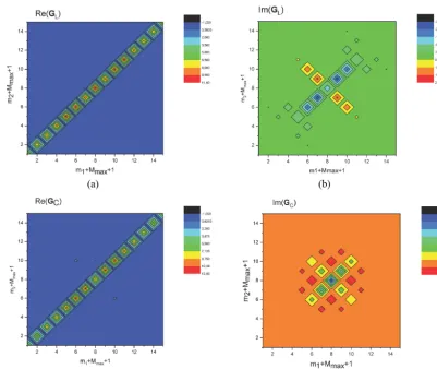
Figure 4.The real part of the matrixGLfor the circular wire.k=
2.3/R.
(Fig. 2). The parameters of the structure are: R=4 m and r0=1 cm. The matrixes GC(k) and GL(k) are calculated
by double integration and partially presented in Figs. 4–6. Using the exact calculations this matrix must be diagonal (see Eqs. 8–10). The relative value of the off-diagonal el-ements relative to diagonal elel-ements represents the error of the method (about 10−3–10−4). But practically, the matrixZ0 is diagonal and coincides with the exact result. The determi-nant of this matrix has minimum approximately forx≈m1 (see Fig. 3 for the inverse value, which has maximums).
The comparison of the values of the poles of the first layer obtained using the numerical algorithm described above with the solution of the exact Eq. (12b) obtained by Maple soft-ware has shown excellent agreement (Table 1). Note that for corresponding values of the parameters of the circular loop the values of the SEM poles of the first layer obtained by the
1The determinant can be a large value in dependence of the order or the matrix. For theMmax=7 its value can reach 1014–1015
Figure 5.The real part of the matrixGCfor the circular wire.k=
2.3/R.
Figure 6.The real part of the matrixZ0for the circular wire.k=
2.3/R.
two methods described above coincide with these one ob-tained earlier by Umashankar and Wilton (1974).
4.2 Short-circuited semi-elliptical wire
As the second example, we consider the semi-elliptical short-circuited wire above a perfectly conducting ground (Fig. 7).
The parameters of the full ellipse (initial wire plus mir-rored wire) are:a=4 m,b=1 m,r0=1 cm.
The matrixesGLandGC are presented in Fig. 9 for real
k. For non-symmetrical configurations, these matrices are not diagonal. However, for the smooth wire (λ|dR(l)/dl| |R(l)|, whereR(l)is the radius of curvature of the wire) the number of essential non-diagonal elements is not too big. This can be observed in Fig. 9, especially for the real parts. For the imaginary parts, the non-diagonal elements are es-sential.
calcu-Table 1.SEM poles of the first layer for the circular wire.
Number of the polem 1 2 3 4 5
Exact solution withgm Re(xm) 1.036 2.050 3.0593 4.0670 5.0736
Im(xm) 7.00×10⁻² 1.0077×10⁻¹ 1.2415×10⁻¹ 1.4388×10⁻¹ 1.6133×10⁻¹
Method of modal parameters Re(xm) 1.0342 2.0446 3.0514 4.0565 5.0606
Im(xm) 6.988×10⁻² 1.0029×10⁻¹ 1.2333×10⁻¹ 1.3912×10⁻¹ 1.5979×10⁻¹
Figure 7.Short-circuited semi-elliptical wire.
Figure 8.Function 1/|F (x, x)|for the elliptical wire.
lations. If one looks carefully at the numerical data for the matrixGC(see Fig. 9c, d), one can see that:
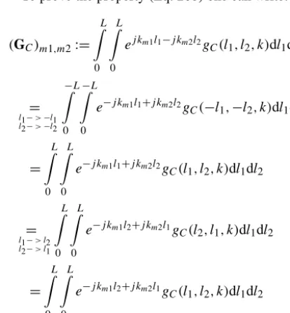
(GC)−m1,−m2=(GC)m1,m2; (20a) (GC)m2,m1=(GC)m1,m2 (20b) The same is true for the matrixesGL(k)andZ(k). This can
be proven in the general case. From the definition ofGC(k)
we have
(GC)m1,m2=
L
Z
0
L
Z
0
ej km1l1−j km2l2g
C(l1, l2, k)dl1dl2
= l1−> l2 l2−> l1
L
Z
0
L
Z
0
ej km1l2−j km2l1g
C(l2, l1, k)dl1dl2
=
L
Z
0
L
Z
0
ej km1l2−j km2l1g
C(l1, l2, k)dl1dl2
=(GC)−m2,−m1 (21)
Here we used the symmetry property of the scalar Green function when rearranging the arguments gC(l2, l1, k)= gC(l1, l2, k).
To prove the property (Eq. 20b) one can write:
(GC)m1,m2:=
L
Z
0
L
Z
0
ej km1l1−j km2l2g
C(l1, l2, k)dl1dl2
= l1−>−l1 l2−>−l2
−L
Z
0 −L
Z
0
e−j km1l1+j km2l2g
C(−l1,−l2, k)dl1dl2
=
L
Z
0
L
Z
0
e−j km1l1+j km2l2g
C(l1, l2, k)dl1dl2
= l1−> l2 l2−> l1
L
Z
0
L
Z
0
e−j km1l2+j km2l1g
C(l2, l1, k)dl1dl2
=
L
Z
0
L
Z
0
e−j km1l2+j km2l1g
C(l1, l2, k)dl1dl2
=(GC)m2,m1 (22)
Here we use also the fact of the even number of integrations and the periodic property of all considered functions.
The results of Eqs. (21) and (22) prove the suggestion Eq. (20).
Figure 9.MatricesGL(a, b)andGC(c, d)for semi-elliptical short-circuited wire.kL/2π=2/3.
has its minimum forx≈m(see Fig. 8 for the inverse value, which has its maximums). This value serves as a zero-order iteration in the algorithm described above. Using this algo-rithm, the SEM poles of the first layer were found (Fig. 10). To check the developed method, we compared the results with the SEM poles obtained from the frequency response function of the line obtained using MoM NEC (Numerical Electromagnetic Code) software. The SEM poles can be ex-tracted from numerical data using a Padé approximation, as described by Senior and Pond (1981). The comparison of the poles obtained by the Method of Modal Parameters and pro-ceeding of the data of NEC calculation is shown in Fig. 10.
The comparison of the SEM poles for the semi-elliptical wire with the poles for the semi-circular wire with similar length is shown in Fig. 11. One can see that the imaginary part for the semi-circular wire is essentially larger relative to the semi-elliptical wire. Both sets of poles have a practi-cally linear dependence from the real part. We believe that this is because, in the case of prolate semi-elliptical config-uration, the horizontal part of the wire is much closer to the conductive surface, which leads to a weaker radiation, which is ultimately responsible for the appearance of the imaginary part of the SEM poles.
Figure 10.SEM-poles for semielliptical configuration obtained by modal parameter method and by analysis of NEC data.
4.3 Straight horizontal wire with short-circuited risers
Figure 11.SEM-poles for semi-circle and semi-elliptical structures.
Lellips=Lcircle=17.1568 m.
Figure 12.Straight horizontal wire with short-circuited risers.
Vance configuration, because it appears in the book of Ed-ward Vance (1978). The parameters of the line are (Fig. 12): Lhor=10 m,h=0.5 m,r0=1 cm.
The matrixes GC andGL for this configuration are
pre-sented in Fig. 14. As in the previous example with the prolate elliptic wire, these matrixes contain non-diagonal elements, which, however, are larger than in the previous case, because of the non-smoothness of the line. Nevertheless, the proper-ties of the matrixes (Eqs. 20a, b) are still valid.
The frequency dependence of the inverse determinant of the matrixZ(which is also non-diagonal) is shown in Fig. 13. As in the previous cases, it has its maximums nearmeff:= kL/2π≈m (m= ±1,±2, . . .), which approximately corre-spond to the real parts of the SEM poles.
Knowledge of the determinant, as a function of complex wave number k, gives us the possibility to determine the SEM poles using the algorithm described above. To check the modal parameter method we compared the results with the one obtained by two alternative methods: the analysis of the response function obtained by NEC (Senior and Pond, 1981), and the asymptotic method (see Tkachenko et al., 2014; Mid-delstaedt et al., 2016). The results are presented in Fig. 15.
Analyzing the results, we can draw several conclusions. First, the agreement with the “exact” numerical results, as well as with the approximate analytical method is much bet-ter in the case of the elliptic wire. This might be caused by
Figure 13.Function 1/|F (x, x)|for the Vance configuration.
the uniform length division by sub-elements in this case, un-like the case of the ellipsoid. In the last case, the uniform division is applied to the parameter t in the usual parametric representation of the ellipse, which leads to a non-uniform division of the lengths of sections of integration and, as a re-sult, the incorrect integration near the singular point at the given number of sub elements (10 000). However, this defi-ciency can be easily corrected in future calculations.
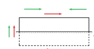
Another important observation is related to the excitation of two types of modes: the common mode and differential mode. The differential mode (m=∼0, 2, 4, . . . , see Fig. 15) appears for any transmission line structure, which has hori-zontal components. The common mode (m=∼1, 3, 5, . . . , see Fig. 15) appears for the transmission line structure, which has vertical elements and excited, for example, by an external field, which has vertical components. Note that both types of modes appear in the two previous examples: semi-circular wire and semi-elliptical wire above the perfectly conduct-ing ground with a non-symmetrical excitation. In the case of the wire without vertical components (horizontal open-circuit line above ground), or in the case of a symmetrical configuration (all three considered configurations) and exci-tation (i.e., plane wave with normal incidence or with grazing incidence), we can observe only one mode type (differential modes or common modes).
Figure 14.MatricesGL(a, b)andGC(c, d)for a straight horizontal wire with short-circuited risers.kL/2π=2/3.
Figure 15.SEM-poles for the Vance configuration obtained by the modal parameter method, by the asymptotic approach and by anal-ysis of NEC data.
by the diagonal matrix element of the modal impedance per-unit length with the modal functions. It is possible to show that this result can also be obtained by the variation method
Figure 16. Differential (red color) and common (green color) modes for the Vance structure.
(Myers et al., 2011a, b). These problems will be addressed in future work.
5 Conclusion
wires, which essentially simplifies finding the poles. The SEM poles are complex roots of the modal impedance matrix of the system. The numerical method of solution of the cor-responding equation was developed and applied for several examples: semi-circular wire, semi-elliptical wire, and hor-izontal wire with vertical risers. During this procedure, ma-trices of modal inductance and capacitance were calculated and their symmetry was investigated. The comparison of the SEM poles with the ones obtained by other analytical and nu-merical methods yields a good agreement. The causes of the disagreement with the numerical results are analyzed. The main cause is using matrices that are not sufficiently large. In our opinion, it possible to improve results by accelerat-ing calculations usaccelerat-ing the symmetry properties of modal ma-trixes (Eqs. 20a, b).
Note, that the MoMP can also be applied for the open-circuited wire if one uses a different modal function (sine and cosine). In the future, the developed method can be gen-eralized for the case of a loaded wire by including the lumped impedances as current controlled voltage sources.
Data availability. Data is available upon request.
Author contributions. SVT was responsible for the development of the method of modal parameters, the idea about application of the MoMP for the calculation of SEM poles, the development of the corresponding analytical method and software, discussion of the re-sults, and writing the text. JBN was responsible for the method of modal parameters, the idea about application of the MoMP for the calculation of SEM poles, carrying out the analytical calculations, discussion of the results, and writing the text. FM was responsi-ble for checking the results both analytically (asymptotic approach and the equations for the reflection coefficients) and numerically (method of moments and the software for the asymptotic approach), discussion of the results, and writing the text. RR had the idea about application of the MoMP for the calculation of SEM poles and con-tributed to the discussion of the results and writing the text (Intro-duction and Conclusion). MS had the idea about application of the MoMP for the calculation of SEM poles and contributed to the dis-cussion of the results and writing the text (Introduction and Con-clusion). RV had the idea about application of the MoMP for the calculation of SEM poles and contributed to the discussion of the results and writing the whole text.
Competing interests. The authors declare that they have no conflict of interest.
Special issue statement. This article is part of the special issue “Kleinheubacher Berichte 2018”. It is a result of the Klein-heubacher Tagung 2018, Miltenberg, Germany, 24–26 September 2018.
Review statement. This paper was edited by Frank Gronwald and reviewed by Andres Gallego and one anonymous referee.
References
Baum, C. E.: On the singularity expansion method for the solu-tion of electromagnetic interacsolu-tion problems, Interacsolu-tion Notes, Note 88, available at: http://ece-research.unm.edu/summa/notes/ In/0088.pdf (last access: 4 August 2019), 1971.
Baum, C. E., Giri, D. V., and Tesche, F. M. (Eds.): The Singularity Expansion Method in Electromagnetics: A Summary Survey and Open Questions, Lulu Enterprises, North Carolina, USA, 2012. Blackburn, R. F.: Analysis and synthesis of an
impedance-loaded loop antenna using the singularity expansion method, Sensor and Simulation Notes, Note 214, available at: http: //ece-research.unm.edu/summa/notes/SSN/note214.pdf (last ac-cess: 4 August 2019), 1976.
Blackburn, R. F. and Wilton D. R.: Analysis and synthesis of an impedance-loaded loop antenna using the singularity expansion method, IEEE T. Antenn. Propag., 26, 136–140, https://doi.org/10.1109/TAP.1978.1141787, 1978.
Giri, D. V. and Tesche, F. M.: An of the natural frequencies of a straight wire by various methods, IEEE T. Antenn. Propag., 60, 5859–5866, https://doi.org/10.1109/TAP.2012.2211317, 2012. Krauthauser, H. G., Nitsch, J., Tkachenko, S., Korovkin, N., and
Scheibe, H.-J.: Transfer impedance at high frequencies, in Pro-ceedings of the 2005 International Symposium on Electromag-netic Compatibility, Chicago, IL, USA, 8–12 August 2005, 228– 233, https://doi.org/10.1109/ISEMC.2005.1513505, 2005. Middelstaedt, F., Tkachenko, S. V., Rambousky, R., and Vick, R.:
High-frequency electromagnetic field coupling to a long, finite wire with vertical risers above ground, IEEE T. Electromagn. C, 58, 1169–1175, https://doi.org/10.1109/TEMC.2016.2544110, 2016.
Middelstaedt, F., Tkachenko, S. V., and Vick, R.: Trans-mission line reflection coefficient including high fre-quency effects, IEEE T. Antenn. Propag., 66, 4115–4122, https://doi.org/10.1109/TAP.2018.2839914, 2018.
Myers, J. M., Sandler, S. S., and Wu, T. T.: Electromagnetic reso-nances of a straight wire, IEEE T. Antenn. Propag., 59, 129–134, https://doi.org/10.1109/TAP.2010.2090479, 2011a.
Myers, J. M., Sandler, S. S., and Wu, T. T.: Electro-magnetic resonances of a straight wire on an earth-air interface, IEEE T. Antenn. Propag., 59, 3154–3164, https://doi.org/10.1109/TAP.2011.2161539, 2011b.
Nitsch, J. B. and Tkachenko, S. V.: Global and modal parameters in the generalized transmission line theory and their physical mean-ing, URSI Radio Sci. Bull., 312, 21–31, 2005.
Nitsch, J. B. and Tkachenko, S. V.: Propagation of current waves along quasi-periodical thin-wire structures: taking radiation losses into account, URSI Radio Sci. Bull., 322, 19–40, 2007. Rachidi, F. and Tkachenko, S. (Eds.): Electromagnetic Field
Inter-action with Transmission Lines: From Classical Theory to HF Radiation Effects, WIT Press, Boston, USA, ISBN 978-1-84564-063-7, 2008.
Mathematical Notes, Note 42, available at: http://ece-research. unm.edu/summa/notes/Mathematics/0042.pdf (last access: 4 Au-gust 2019), 1976.
Senior, T. B. A. and Pond, J. M.: Pole extraction in the fre-quency domain, Interaction Notes, Note 411, available at: http://ece-research.unm.edu/summa/notes/In/0411.pdf (last ac-cess: 4 August 2019), 1981.
Tesche, F. M., Ianoz, M. V., and Karlsson, T.: EMC Analytical Methods and Computational Models, Willey&Son, NY, USA, ISBN 0-471-15573-X, 1997.
Tkachenko, S. and Nitsch, J.: On the Electromagnetic Field Excitation of Smoothly Curved Wires, in: Proceedings of the VI International Symposium on Electromag-netic Compatibility and ElectromagElectromag-netic Ecology (EMC-2005), St.-Petersburg, Russia, 21–24 June 2005, 115–120, https://doi.org/10.1109/EMCECO.2005.1513078, 2005. Tkachenko, S., Rachidi, F., and Ianoz, M.: High-frequency
electro-magnetic field coupling to long terminated lines, IEEE T. Elec-tromagn. C., 43, 117–129, https://doi.org/10.1109/15.925531, 2001.
Tkachenko, S., Nitsch, J., and Rambousky, R.: Electromagnetic field coupling to transmission lines inside rectangular resonators, Interaction Notes, Note 623, available at: http://www.ece.unm. edu/summa/notes/In/IN623.pdf (last access: 4 August 2019), 2011.
Tkachenko, S. V., Nitsch, J., Vick, R., Rachidi, F., and Pol-jak, D.: Singularity expansion method (SEM) for long termi-nated transmission lines, in Proceedings of the 2013 Inter-national Conference on Electromagnetics in Advanced Appli-cations (ICEAA), Torino, 9–13 September 2013, 1091–1094, https://doi.org/10.1109/ICEAA.2013.6632411, 2013.
Tkachenko, S., Middelstaedt, F., Nitsch, J., Vick, R., Lu-grin, G., and Rachidi, F.: High-frequency electromagnetic field coupling to a long finite line with vertical risers, in Proceedings of the 2014 XXXIth URSI General As-sembly and Scientific Symposium (URSI GASS), Beijing, https://doi.org/10.1109/URSIGASS.2014.6929526, 2014. Tkachenko, S. V., Nitsch, J. B. Middelstaedt, F., Magdowski, M.,
Hellge-Theune, D., Sheibe, H.-J., Rambousky, R., and Vick, R.: Application of singularity expansion method (SEM) to nonuni-form transmission lines, in Proceedings of European Electromag-netics Symposium EUROEM 2016, 11–14 July 2016, London, UK, available at: http://ece-research.unm.edu/summa/notes/ AMEREM-EUROEM/EUROEM2016BookofAbstracts.pdf (last access: 4 August 2019) (37Mb), 2016.
Umashankar, K. R. and Wilton, D. R.: Transient characterization of circular loop using singularity expansion method, Interac-tion Notes, Note 259, available at: http://ece-research.unm.edu/ summa/notes/In/0259.pdf (last access: 4 August 2019), 1974. Wu, T. T.: Theory of the thin circular loop antenna, J. Math. Phys.,
3, 1301–1304, https://doi.org/10.1063/1.1703875, 1962. Vance, E.: Coupling to Shielded Cables, Willey&Son, NY, USA,