Recent global CO 2ﬂux inferred from atmospheric CO2 observations and its regional analyses

(1)

www.biogeosciences.net/8/3263/2011/ doi:10.5194/bg-8-3263-2011

Biogeosciences

Recent global CO

2

flux inferred from atmospheric CO

2

observations and its regional analyses

F. Deng and J. M. Chen

Department of Geography, University of Toronto, Canada

Received: 24 February 2011 – Published in Biogeosciences Discuss.: 1 April 2011

Revised: 30 September 2011 – Accepted: 20 October 2011 – Published: 11 November 2011

Abstract. The net surface exchange of CO2 for the years

2002–2007 is inferred from 12 181 atmospheric CO2

con-centration data with a time-dependent Bayesian synthesis in-version scheme. Monthly CO2fluxes are optimized for 30

re-gions of the North America and 20 rere-gions for the rest of the globe. Although there have been many previous multiyear in-version studies, the reliability of atmospheric inin-version tech-niques has not yet been systematically evaluated for quanti-fying regional interannual variability in the carbon cycle. In this study, the global interannual variability of the CO2flux

is found to be dominated by terrestrial ecosystems, particu-larly by tropical land, and the variations of regional terrestrial carbon fluxes are closely related to climate variations. These interannual variations are mostly caused by abnormal mete-orological conditions in a few months in the year or part of a growing season and cannot be well represented using annual means, suggesting that we should pay attention to finer tem-poral climate variations in ecosystem modeling. We find that, excluding fossil fuel and biomass burning emissions, terres-trial ecosystems and oceans absorb an average of 3.63±0.49 and 1.94±0.41 Pg C yr−1, respectively. The terrestrial up-take is mainly in northern land while the tropical and south-ern lands contribute 0.62±0.47, and 0.67±0.34 Pg C yr−1 to the sink, respectively. In North America, terrestrial ecosystems absorb 0.89±0.18 Pg C yr−1on average with a strong flux density found in the south-east of the continent.

1 Introduction

The steady increase of atmospheric CO2 during the past

200 yr is believed to be the major contributor to the warming of the climate system. However, in the past half century only

Correspondence to: F. Deng

([email protected])

about 40 % of the anthropogenic emissions has remained in the atmosphere (Jones et al., 2005; Canadell et al., 2007); the remainder has been absorbed by the oceans and/or fixed by the terrestrial biosphere. Information on the spatial and temporal distribution of the carbon flux is critical to under-standing and managing, if possible, the global carbon cycle to prevent potentially catastrophic climate change.

Global atmospheric CO2concentration observations have

been one of the most important datasets in quantifying and understanding the global carbon cycle. In the early years, scientists utilized the measurements from limited sites to an-alyze the temporal variability of the global carbon cycle. As more sites are added to the global observation network, in-verse techniques have been developed to understand both the temporal and spatial distributions of carbon exchange across the surface of the globe.

The Bayesian synthesis inversion (Enting et al., 1995) and its variants have been used extensively in estimating global or regional CO2fluxes (e.g., Fan et al., 1998; Rayner et al.,

1999; Ciais et al., 2000; Gurney et al., 2002, 2003; Law et al., 2003). In recent years, the progress of inversion has been made in two directions (Gurney et al., 2008): (i) estimating fluxes with finer spatial resolutions (Kaminski et al., 1999; R¨odenbeck et al., 2003; Peters et al., 2005, 2007; Mueller et al., 2008; Lokupitiya et al., 2008) and (ii) understanding the magnitude and possible mechanisms of interannual vari-ability (e.g., Bousquet et al., 2000; R¨odenbeck et al., 2003; Peylin et al., 2005; Patra et al., 2005; Baker et al., 2006; Bruhwiler et al., 2007; Gurney et al., 2008; Rayner et al., 2008; Peters et al., 2010). Although different inversions gen-erally agree on flux estimates at the hemisphere scale, large discrepancies still exist at the regional scale because of the limitations in observations used, models employed, and other setups of these inversions.

Considering the fact that inverse techniques compare the spatiotemporal distributions of simulated CO2

(2)

with observations at discrete sites over the globe, more con-tinental observations should be used to estimate terrestrial CO2 fluxes at a sub-continental scale. Deng et al. (2007)

attempted to use observations at continental sites to pursue a CO2inversion for 30 regions in North America, but large

diurnal variations of the planetary boundary layer (PBL) at continental sites could have caused large diurnal variations of CO2concentration and hence produced substantial biases

in the inversion result, since a transport model without con-sidering the diurnal variations was used. Besides the diurnal PBL variation, terrestrial ecosystems, themselves often en-hance the diurnal cycle of CO2concentration in the growing

seasons by assimilating CO2 from the ambient atmosphere

during the daytime, while exhaling CO2 to the atmosphere

during night-time. Therefore, a transport model with diur-nally variable biosphere fluxes and planetary boundary layer dynamics is needed to minimize the biases.

Understanding the feedbacks between the carbon cycle and the climate system is critical for projecting change in climate. Several atmospheric inversion experiments (e.g., Rödenbeck et al., 2003; Peylin et al., 2005; Baker et al., 2006; Gurney et al., 2008; Rayner et al., 1999, 2005, 2008) have shown that the interannual variability of inverted fluxes could be reasonably explained by extreme climate and other events, such as El Niño/La Niña-Southern Oscillation (ENSO), and the eruption of Mt. Pinatubo in 1991. Further investigation of the relationships of the inverted fluxes with climatic conditions at a regional scale would assist us indi-rectly evaluating the inversion results, especially the variabil-ity of the inverted fluxes, on the one hand, and improve our understanding of how the carbon cycle could respond to the change in climatic conditions, on the other hand.

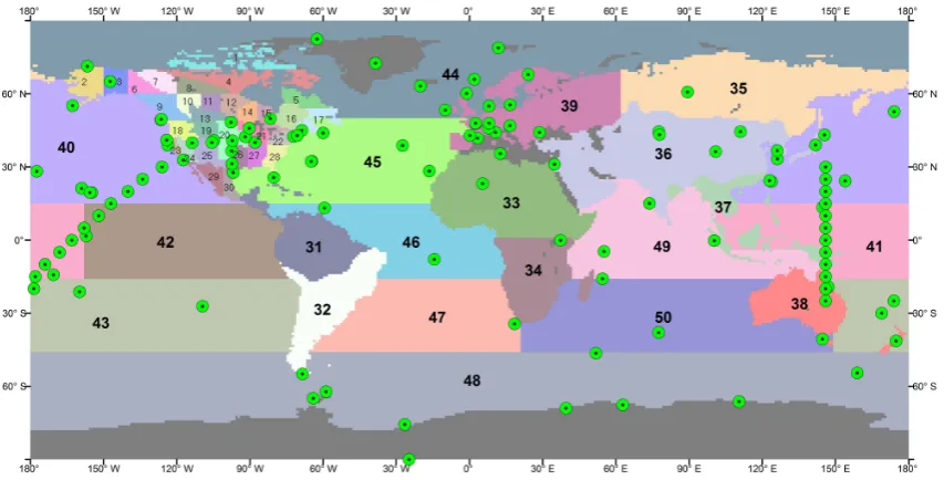
In this study, we continue monthly inversion based on the Bayesian principle, for estimating carbon fluxes of 30 re-gions in North America and 20 rere-gions for the rest of the globe (Fig. 1) (Deng et al., 2007) and extend it to a 6 yr (2002–2007) period. Both the seasonal and diurnal rectifier effects (Denning et al., 1996) are also considered. Through this inversion, we will make an effort to (i) improve the esti-mation of the spatial distribution of CO2sources and sinks

and their uncertainties over the Earth’s surface, especially over North America, (ii) examine the interannual variability of the global CO2flux and locate the main source of the

vari-ability, and (iii) observe if the inferred flux variations (sea-sonal, and interannual) could be explained by climatic con-ditions and their anomalies in terms of complying with our understanding of the terrestrial ecosystem process.

The remainder of this paper is organized as follows. Sec-tion 2 provides a brief explanaSec-tion of the methodology and datasets used for the inversion and climatic data used to ana-lyze the inverted terrestrial carbon fluxes. Section 3 presents the major results in three areas: (i) the spatial distribution of carbon sources and sinks, (ii) the interannual variability of the fluxes, and (iii) the link between inverted regional fluxes and climatic conditions. In Sect. 4, we compare the results of

our inversion with bottom-up modeling and other inversions, and highlight the importance of climate anomalies at finer temporal resolution for terrestrial carbon cycle modeling.

2 Data and methods

2.1 Inversion method and data

The inversion technique used in this study is the time-dependent Bayesian inversion considering both the diurnal variations of the atmospheric boundary layer dynamics and the surface CO2exchange. The inversion problem reduces to

minimizing the cost function (Enting et al., 1995; Rayner et al., 1999)

J=1

2(Ms−c)

T_R−1₍_M_s−c)₊1

2(s−sp)

T_Q−1_(s−s

p). (1)

Where M is a matrix representing a transport (observation) operator;cis a vector of the observations; sis an unknown vector of the carbon flux of all regions to be inverted at dif-ferent times combined with the assumed initial well-mixed atmospheric CO2concentrations;spis the a priori estimate

ofs; and uncertainties ofcandspare expressed in covariance

matrixes R and Q.

We employ the sum of squares of normalized residuals from fit (χ2test) (Gurney et al., 2003) to test the consistency of the fit to data and prior flux estimates simultaneously.

Transport of the atmospheric CO2 is simulated using

the global two-way nested transport model TM5 (Krol et al., 2005), an offline model driven by meteorology from the European Centre for Medium-Range Weather Forecasts (ECMWF) model. In this study, TM5 is run at a 6×4◦

res-olution globally with a nested 3×2◦ _{resolution over North}

America.

The selection of a proper atmospheric transport model would be critical to the accuracy of inversion as transport models can make considerable differences in the inverted car-bon flux. However, the differences are mostly in the absolute flux values for a given region, and the patterns of the seasonal and inter-annual variations are similar if adequate measure-ments are used (Baker et al., 2006). In addition, the transport of TM5 has been extensively evaluated (Peters et al., 2004; Krol et al., 2005) and TM5 performs consistently well in at-mospheric transport model intercomparisons (Stephens et al., 2007; Peters et al., 2007).

A total of 4800 forward model simulations were conducted in this study to form the transport (observation) operator (M)

of eight years (2000–2007) for the 50 regions. For each month and region, a flux of 1 Pg C was prescribed in the TM5 model for forward transport computation to determine the contribution of each region to the CO2concentration at

each observation site in order to form the M matrix. Further-more, to invert the monthly CO2flux in a framework that the

(3)

[image:3.595.85.512.61.278.2]

Fig. 1. An inversion scheme: 30 regions in North America and 20 regions for the rest of the globe. Locations of 210 CO₂observational sites are also indicated.

continental sites. For tower sites, afternoon hours were sam-pled to avoid the error-prone simulations under extremely stable and stratified nocturnal atmospheric conditions near the ground. For non-tower continental sites, the fraction of the total number of samples collected within each hour has been used as a weight in modifying the monthly transport (observation) operator (M). The same weight was also used to sample the pre-subtracted portions of CO2concentration

discussed below.

Monthly CO2 concentration observation data of 7 yr

(2001–2007) were compiled from the GLOBALVIEW-CO2

2008 database. Though the GLOBALVIEW-CO2 database

consists of both extrapolated and interpolated data that were created based on the technique devised by Masarie and Tans (1995), we chose the synchronized and smoothed values of actual observations to compile our own CO2concentration

dataset. CO2concentration data of 2001 to 2007 at 210 sites

(Fig. 1) were used in this study.

Four background fluxes were considered through another set of forward transport model simulations to calculate the pre-subtracted portions of the CO2 concentration in order

to minimize of the nonlinear effects of the large basis re-gions (Pickett-Heaps, 2007). These fluxes include (i) the fos-sil fuel emission field (http://carbontracker.noaa.gov), which was constructed based on (a) the global, regional and na-tional fossil-fuel CO2emission inventory from 1871 to 2006

(CDIAC) (Marland et al., 2009) and (b) the EDGAR 4 database for the global annual CO2 emission on a 1×1◦

grid (Olivier and Berdowski, 2001); (ii) the hourly terrestrial ecosystem exchange produced by BEPS (Chen et al., 1999), which was driven by NCEP reanalyzed data (Kalnay et al., 1996) and remotely sensed LAI (Deng et al., 2006), and a

special treatment was taken to neutralize the annual flux at each grid; (iii) the flux of CO2across the air-water interface

constructed based on the results of daily CO2fluxes using the

OPA-PISCES-T model forced by daily wind stress and heat and water fluxes from the NCEP reanalyzed data for 2000 to 2007 (Buitenhuis et al., 2006); and (iv) the monthly mean fire emission available from the Global Emissions Fire Database version 2 (GFEDv2) (Randerson et al., 2007; van der Werf et al., 2006). Therefore, the vectorcin Eq. (1) can further be expressed as

c=cobs−cff−cbio−cocn−cfire (2)

wherecobsis the monthly CO2concentration derived from

GLOBALVIEW-CO2;cff,cbio,cocn, andcfire are simulated

CO2concentrations from fluxes (i), (ii), (iii), and (iv),

respec-tively.

The model-data mismatch reflects the difference between observations and modeled results, which incorporates errors associated with observations (instrument errors) and errors from the modeling of the observations. Various approaches (Rayner et al., 1999; R¨odenbeck et al., 2003; Baker et al., 2006; Michalak et al., 2005; Bruhwiler et al., 2007) have been used to determine the model-data mismatch error. As pointed out by Bruhwiler et al. (2007), choosing the appro-priate values for the model-data mismatch error is difficult because there are insufficient independent data available for detailed model evaluations at each observation site. We used a method based on the category similar to that of Peters et al. (2005) and Baker et al. (2006). We divided the obser-vation sites into 5 categories, each with its own assigned constant portion (σconst)and a variable portion (GVsd) that

(4)

residual distribution of the average monthly variability (var) files of GLOBALVIEW-CO22008. Then the mismatch error

covariance as a diagonal matrix, R, can be defined with the error standard deviation of monthias

Rii=σconst2 +GVsd2. (3)

The categories and respective σconst are: Antarctic sites

(0.15), oceanic sites (0.30), land and tower sites (1.25), mountain sites (0.90), and aircraft samples (0.75). These were designed to reflect the systematic simulation errors for each category of sites.

Significant vertical error correlations exist between differ-ent levels at tower sites and aircraft samplings. The ensem-ble model simulations (Lauvaux et al., 2009) are not read-ily applied to global-scale inversion, and improperly defined covariances could lead to unrealistic corrections of inverted fluxes. Therefore, we inserted a weighting factor (W)into the cost function (Eq. 1) as

J=1

2(W(Ms−c))

T_R−1₍_W₍_M_s₋_c))

+1

2(s−sp)

T_Q−1_(s₋_s

p) (4)

to compensate for the effect that several similar “forcings” act in the cost function, which could cause significant biases in regional CO2fluxes if they are not restricted. We

conser-vatively define the diagonal matrix (W)with item

wii=1/(1+0.6(n−1)) (5)

wherenis the number of observations at different levels, in the same geographical location.

The prior flux estimates for both oceans and lands in this study were prescribed as zero after we subtracted the contri-butions to the CO2concentration from (i) the ocean surface

CO2exchange, (ii) the fossil fuel emission, (iii) the terrestrial

ecosystem carbon exchange, and (iv) the biomass burning. There are many sources of uncertainty in the air-sea CO2

flux, including the error of reanalyzed meteorological data, the error of the estimated parameters in the OPA-PISCES-T model, and the error caused by the model itself. Therefore, estimating the uncertainties of the model outputs is extremely difficult. The spread (0.5 Pg C yr−1_{) of ocean uptakes in four}

ocean models (Le Quéré et al., 2007; Lovenduski et al., 2008; Rodgers et al., 2008; Wetzel et al., 2005) provides a good ref-erence of uncertainty in bottom-up modeling. Rödenbeck et al. (2003) also used 0.5 Pg C yr−1as his prior global ocean flux uncertainty. Considering that the a priori used in this study is at upper bound of those four ocean uptakes, we used an uncertainty of 0.67 Pg C year−1, distributed among 11 ocean regions according to Baker et al. (2006).

As shown in Eq. (2), the contributions to the atmospheric CO2concentration of the four background fluxes have been

removed from the observations, thus the fluxes we are going to infer directly from Eq. (4) are the residual fluxes after the

background fluxes are subtracted, as discussed by R¨odenbeck et al. (2003). The sources of uncertainty in the land surface flux are more complicated than that of the air-sea surface ex-change. Fossil fuel emissions have small uncertainties (±6 % of the global fossil fuel emissions, Marland, 2008) that are often not considered in atmospheric inversions. Gurney et al. (2005) demonstrated that ignoring the uncertainties of fos-sil fuel emissions in time and space could effectively bias the seasonal pattern of surface fluxes and significantly change the distribution of inverse fluxes in a high resolution inver-sion. The estimates of vegetation fire emissions are uncertain to about 20 % (1σ )on global, annual scales (van der Werf et al., 2010). Similar to fossil fuel emissions, the uncertain-ties of vegetation fires could not be handled separately in this study. It should, however, be noted that any inverse estimate of the terrestrial carbon flux excluding fire emissions and fos-sil fuel emissions could be biased by these uncertainties. Be-sides the aforementioned error in the spatiotemporal distribu-tion of emissions from fossil fuel combusdistribu-tion and vegetadistribu-tion fires, the heterogeneous distributions of carbon assimilation and respiration of terrestrial ecosystems in both space and time are more error-prone. Bearing these in mind, we used an uncertainty of 2.0 Pg C yr−1(based on a similar regional scheme of TRANSCOM 3) for the global land surface that was spatially distributed based on the annual NPP distribu-tion simulated by BEPS.

The prior uncertainties for global land and ocean assigned in this study are in the range of those used in previous studies (e.g., Baker et al., 2006; Bruhwiler et al., 2007; Gurney et al., 2004; R¨odenbeck et al., 2003). Aχ2test indicates that these uncertainties are reasonable.

2.2 Climate data

The Global Precipitation Climatology Centre (GPCC) pro-vided a gridded monthly precipitation product for the global land surface. The GPCC’s Full Data Reanalysis Version 4 (Schneider et al., 2008) is available for 1901–2007 with a resolution of 0.5◦. A global monthly land surface air tem-perature dataset (Fan and van den Dool, 2008), at 0.5×0.5◦ resolution, covers the global land areas for the period from 1948 to present. It is based on a combination of the Global Historical Climatology Network Version 2 and the Climate Anomaly Monitoring System datasets.

The regional annual averages, monthly, and 3-monthly values and anomalies of air temperature and precipitation for 6-yr (2002–2007) are closely examined to find the links be-tween the variation of inverted CO2fluxes and climatic

(5)

[image:5.595.50.286.66.363.2]

Fig. 2. Map of mean posterior carbon flux for 2002-2007 derived in

this study, (a) excluding fossil fuel and biomass burning emissions, and (b) excluding only fossil fuel emissions. The a priori ocean exchange and biomass burning emission are considered at 1×1◦ resolution.

3 Results

3.1 Six-year mean fluxes

Figure 2a and b show the two mean CO2flux maps for 2002–

2007. Only the pre-subtracted biosphere fluxes and the in-verted residual fluxes are included for land regions, while the pre-subtracted ocean fluxes at 1×1◦resolution and the inverted fluxes are aggregated for ocean regions in Fig. 2a. In Fig. 2b, the pre-subtracted biomass burning emissions at 1×1◦resolution are also combined into land regions.

Most of the land regions are inverted as CO2sinks, while

Tropical America (Region 31), Australasia (Region 38), and Region 2 (Alaska) release CO2to the atmosphere. Southern

Africa (Region 34), Boreal Asia (Region 35), Tropical Asia (Region 37), and North America are found to be strong sinks. Tropical and southern hemispheric land regions have been affected by biomass burning significantly.

Focusing on the 30 North America regions, we find the highest uptake area in the eastern US, while an isolated high uptake appears in the far northwest (Region 18). In Canada, relative high uptake is found in Regions 10, 14, 15, and 16,

which is quite consistent with the spatial pattern of forest age (Chen et al., 2003; Pan et al., 2011).

When the land regions are aggregated, the northern land is estimated as a big sink of 2.35±0.25 Pg C yr−1, while tropical and southern lands are estimated as two small sinks of 0.62±0.47 and 0.67±0.34 Pg C yr−1, respectively (in all cases, excluding biomass burning emissions). Tropical and southern lands become two sources of 0.81±0.47, and 0.22±0.34 Pg yr−1, respectively, when biomass burning is taken into account.

The distribution of ocean fluxes is dominated by the back-ground (Buitenhuis et al., 2006) used. The most noticeable difference from the background produced by the inversion appears in the mid-latitude ocean regions of the Southern Hemisphere (Regions 43 – South Pacific, 47 – South At-lantic, and particularly Region 50 – South Indian). These re-gions are inferred here to have more uptake in a belt (around 30◦_{S), while we infer a positive difference from the}

back-ground as large as 0.31 Pg C yr−1 toward a source in the southern ocean (Region 48, south of 45◦S). This is con-sistent with a source of 0.40±0.18 Pg C yr−1 inverted by Mikaloff Fletcher et al. (2007) who employed a suite of 10 different Ocean General Circulation Models (OGCMs). In contrast, Le Qu´er´e et al. (2007) reported a sink in the 1990s in the region through an atmospheric inversion, al-though the sink becomes weaker significantly after 1990, a trend, they attributed to the increasing wind speeds that may cause more upwelling of C-rich waters from which a higher

pCO2 in the surface water is produced. The new

measure-ments from winter months for this region show that South-ern Ocean surface water pCO2 has been increasing faster

than the atmospheric pCO2 increase rate, which implies a

decreasing sink (Takahashi et al., 2009). Aggregated ocean fluxes show quite a symmetric distribution pattern: north-ern and southnorth-ern oceans show uptakes of 1.34±0.22, and 1.41±0.22 Pg C yr−1, respectively, while the tropical ocean releases 0.81±0.27 Pg C yr−1to the atmosphere.

Combining these inverted land and ocean fluxes with other background fluxes (emissions from fossil fuel and biomass burnings) used in our inversion, we could get an integrated picture of the global carbon budget. Over the period considered in this study, the global net CO2

emis-sion to the atmosphere is 4.56±0.27 Pg C yr−1, of which the land surface emits 6.25±0.49 Pg C yr−1, and ocean ab-sorbs 1.69±0.41 Pg C yr−1. The land surface budget con-sists of roughly 7.33, 2.56, and−3.63 Pg C yr−1 _from

fos-sil fuel emission, biomass burning, and terrestrial ecosys-tem uptake, respectively, while fossil fuel burning emits 0.25 Pg C yr−1over the ocean surface and the ocean uptake is around 1.95 Pg C yr−1.

Figure 3 summarizes the mean global CO2 budget of

(6)

[image:6.595.133.466.65.180.2]

Fig. 3. Mean global carbon budget of 2002–2007 inferred from atmosphere observations. Carbon budgets over land and ocean are partitioned

further based on our inverted fluxes and estimated fluxes from fossil fuels consumption (http://carbontracker.noaa.gov, 2009), biomass burning (Randerson et al., 2007) and ocean uptake (Buitenhuis et al., 2006) (unit: Pg C yr−1).

are shown in the bottom of the figure without explicit uncer-tainties.

3.2 Interannual variations

The inverted CO2fluxes (excluding emissions from fossil

fu-els consumption and biomass burning) from 2002 to 2007 at the regional level are shown in Fig. 4. The results of 30 small North American regions are shown in Fig. 4a (Regions 1 to 17), and Fig. 4b (Regions 18 to 30), and the results of the larger land and ocean regions are illustrated in Fig. 4c and d, respectively.

The interannual variabilities (IAVs) of North America re-gions are relatively small. Of all the small rere-gions (Fig. 4a and b), only three show a difference between the maximum and minimum (herein below, this difference is referred to as IAV) larger than 0.1 Pg C yr−1_{, and all of them appear in}

east-ern US. The two aggregated North American regions, NA-N (Regions 1–17) and NA-S (Regions 18–30), sustain negative fluxes (sinks) for six-year with small IAVs (Fig. 4c).

Of other large terrestrial regions (Fig. 4c), 7 regions (all except Regions 37 and 38) have large IAVs of more than 0.6 Pg C yr−1. Tropical America (Region 31), South Amer-ica (Region 32), and Europe (Region 39), swing between negative and positive fluxes and show IAVs of 1.15, 0.98, and 0.85 Pg C yr−1, respectively.

Ocean regions (Fig. 4d) show much smaller IAVs than land regions. 10 of them show IAVs of less than 0.5 Pg C yr−1, while the South Pacific region (Region 43) is inverted with an IAV of 0.62 Pg C yr−1. In contrast to land regions, ocean regions with large IAVs do not switch the direction of the fluxes, revealing that the distribution pattern of the ocean CO2flux is stable at this spatiotemporal scale.

Similar to other studies (e.g., Baker et al., 2006), our in-verted fluxes have been aggregated to three land regions, three ocean regions (Fig. 5a), and further to land, ocean, and global scale (Fig. 5b). We see a global IAV of 2.55 Pg C yr−1, while land and ocean, maintaining CO2uptake, show IAVs

of 3.08 and 1.35 Pg C yr−1, respectively. Tropical land switches between uptake and release of CO2 with an IAV

of 2 Pg C yr−1, while both Northern land and Southern land continue to absorb CO2with lower IAV values of 0.92 and

0.51 Pg C yr−1, respectively. Steady zonal distributions of the ocean fluxes are well revealed in Fig. 5a, while the trop-ical ocean release CO2 to the atmosphere with an IAV of

0.45 Pg C yr−1_{, and both northern and southern oceans}

ab-sorb CO2with their IAV values of 0.70 and 0.63 Pg C yr−1,

respectively.

A regression of the annual global fluxes with the annual land fluxes shows that 81 % of the global IAV could be ex-plained by the IAV of land fluxes, whereas ocean fluxes could only explain 4 % of the global variance. Further analysis shows that the IAV of global annual CO2 fluxes is likely

dominated by the IAV of the CO2 fluxes in tropical land

(R2=0.76), compared to northern land (R2=0.40) and southern land (R2=0.36). The IAVs of three aggregated ocean regions could hardly explain the global IAV, while northern and tropical ocean fluxes correlate negatively with the global fluxes, and theR2for the southern ocean is only 0.19.

3.3 Variation of inverted terrestrial fluxes with climatic conditions

(7)

[image:7.595.80.511.60.658.2]

Fig. 4. Inverted CO2fluxes and their uncertainties for 2002 to 2007. (a) Northern North American small regions (1–17), (b) Southern North

(8)

-3.5 -3 -2.5 -2 -1.5 -1 -0.5 0 0.5 1 1.5 2

Land-north Land-tropical Land-south Ocean-north Ocean-tropical Ocean-south

Fl

ux (

P

g

C/

yr

)

(a)

-3.5

Land-north Land-tropical Land-south Ocean-north Ocean-tropical Ocean-south

-8 -7 -6 -5 -4 -3 -2 -1 0

Global Land Ocean

Flux (Pg

C/y

r)

2002 2003 2004 2005 2006 2007

(b) -8

[image:8.595.129.466.64.379.2]

Global Land Ocean

Fig. 5. Aggregated inverted CO2fluxes and their uncertainties from 2002 to 2007 (a) in Northern Land, Tropical Land, and Southern Land,

and in Northern Ocean, Tropical Ocean, and Southern Ocean, and (b) of global total, total land, and total ocean.

co-variations. The 6-yr monthly fluxes and their uncertain-ties, the annual quantiuncertain-ties, and 3-monthly anomalies of the inverted fluxes, air temperature, and precipitation of these regions are shown in Figs. 6–9.

Region NA-N, an aggregated region, including Canada and Alaska, exhibits an IAV of 0.08 Pg C yr−1, an equiva-lent of a third of the average sink inverted for the 6-yr pe-riod (Fig. 6b). 2002 and 2005 are the two years when the inverted annual fluxes substantially departed from the other four years. The positive anomaly of the inverted flux in April–June, 2002 (Fig. 6e) could be attributed to the low temperature that cannot support the normal plant growth. While the inverted annual flux in 2005 shows the largest pos-itive anomaly among the six consecutive years, the cause of this anomaly, however, is quite different from that of 2002. The largest positive flux anomaly in July–September 2005 (Fig. 6e) coincides with a negligible anomaly in tempera-ture (Fig. 6f), and a large positive anomaly in precipitation (Fig. 6g). Normally, we are tending to ascribe a positive flux anomaly to a drought during this season. The fact is that in 2005, Canada experienced its wettest year since reli-able nationwide records commenced in 1948 (Shein, 2006). The wide-spread flood in Manitoba, for example, inundated a quarter of the province’s farmland, and this could

signifi-cantly affect the plant growth and hence the carbon exchange. The most negative anomaly of flux appears in April–June 2006 (Fig. 6e), reconfirming that the thermal condition dur-ing the first half year is crucial to plant growth and carbon uptake in this region.

Region NA-S, an aggregated region, including the con-tiguous United States and Mexico, exhibits an IAV of 0.40 Pg C yr−1, an equivalent of 62 % of the 6-yr mean of the inverted sinks (Fig. 7b). While the inverted annual CO2

uptake in 2002 is the smallest among the 6-yr period, we determine that the main cause of this positive flux anomaly is the negative precipitation anomalies in January–March, April–June, July–September of 2002 (Fig. 7g), in addition to the positive temperature anomalies found in April–June, and July–September (Fig. 7f). Drought induced by low pre-cipitation and high temperature could weaken the ability of plants to assimilate CO2, while high temperature could also

enhance ecosystem respiration. The two larger positive flux anomalies in April–June and July–September of 2002 corre-spond well with the negative precipitation, and positive tem-perature, clearly indicating the links between the inverted carbon flux and climatic conditions. In contrast to Region NA-N, the largest inverted annual CO2sink in this region is

(9)

0 P g C/y r) 0 0.02 0.04 0.06 0.08 y of Flu x (Pg C) Jan‐Mar Apr‐Jun Jul‐Sep Oct‐Dec e ‐0.5 ‐0.4 ‐0.3 ‐0.2 ‐0.1 0 0.1 0.2

2002 2003 2004 2005 2006 2007

Flu x (Pg C/month) Year a -0.3

2002 2003 2004 2005 2006 2007

Flux (P g C/ y Year b 268 268.5 269 269.5 270 270.5 271

2002 2003 2004 2005 2006 2007

T (K ) c 620 640 d ‐0.06 ‐0.04 ‐0.02 0 0.02

2002 2003 2004 2005 2006 2007

An o m aly of Fl u Year Oct Dec ‐2 ‐1.5 ‐1 ‐0.5 0 0.5 1 1.5 2 2.5

2002 2003 2004 2005 2006 2007

An o m aly of T (K ) Year f 20 25 g 20 0 20 0 20 0 20 0 20 0 20 0 Year 500 520 540 560 580 600 620 640

2002 2003 2004 2005 2006 2007

P

(mm)

d

2002 2003 2004 2005 2006 2007

Year ‐20 ‐15 ‐10 ‐5 0 5 10 15 20 25

2002 2003 2004 2005 2006 2007

[image:9.595.122.476.60.538.2]

An o m aly of P (mm) Year g

Fig. 6. The variations of inverted fluxes and climatic conditions from 2002 to 2007 in Region NA-N (Regions 1–17). (a) The inverted

monthly fluxes (thick blue line) and their uncertainties (thin red line), (b) the inverted annual fluxes, (c) the annual mean temperatures,

(d) the annual precipitations, (e) the 3-monthly anomalies of inverted fluxes, (f) the 3-monthly temperature anomalies, and (g) the 3-monthly

precipitation anomalies.

during the first half of the year (Fig. 7e). These negative flux anomalies coincide with the harmonized moisture, thermal conditions in January–March, April–June. The strong nega-tive flux anomaly rarely seen in January–March is mainly a result of the additional carbon uptake in several small south-ern regions. 2006 is the hottest year (Fig. 7c) in the 6-yr period. Contradicting to our expectation, the inverted annual sink is found to be the second to the largest. This may be attributed to the heterogeneity of the terrestrial ecosystems

(10)

-0.3 0 P g C/y r) 0 0.05 0.1 0.15 0.2 y of Flu x (Pg C) Jan‐Mar Apr‐Jun Jul‐Sep Oct‐Dec e ‐0.5 ‐0.4 ‐0.3 ‐0.2 ‐0.1 0 0.1 0.2

2002 2003 2004 2005 2006 2007

Flu x (Pg C/month) Year a -0.9 -0.6

2002 2003 2004 2005 2006 2007

Flux (P g C/ y Year b 286 286.5 287 287.5

2002 2003 2004 2005 2006 2007

T (K ) c 780 800 d ‐0.15 ‐0.1 ‐0.05 0 0.05

2002 2003 2004 2005 2006 2007

An o m aly of Fl u Year Oct Dec ‐1 ‐0.5 0 0.5 1

2002 2003 2004 2005 2006 2007

An o m aly of T (K ) Year f 20 30 g 20 0 20 0 20 0 20 0 20 0 20 0 Year 640 660 680 700 720 740 760 780 800

2002 2003 2004 2005 2006 2007

P

(mm)

d

2002 2003 2004 2005 2006 2007

Year ‐30 ‐20 ‐10 0 10 20 30

2002 2003 2004 2005 2006 2007

[image:10.595.121.476.63.536.2]

Fig. 7. The variations of inverted fluxes and climatic conditions from 2002 to 2007 in Region NA-S (Regions 18–30). (a) The inverted

Region 31: Amazonia is the dominant part of Region 31. While tropical land dominates the global carbon budget in-terannual variation, the changes in Amazonian ecosystems, the planet’s most significant biological repositories of carbon (Grace et al., 2001) are expected to play a key role in both local and global carbon budget variations (Cox et al., 2000). Though the carbon cycle of Tropical America (Amazonia) has been extensively studied, the carbon balance of this re-gion remains highly uncertain. Inverse studies show that this

(11)

0.6 0.9 1.2 P g C/y r) b 0 0.1 0.2 0.3 0.4 y of Flu x (Pg C)

Jan‐Mar Apr‐Jun Jul‐Sep Oct‐Dec

e ‐0.6 ‐0.4 ‐0.2 0 0.2 0.4 0.6

2002 2003 2004 2005 2006 2007

Flu x (Pg C/month) Year a -0.3 0 0.3 0.6

2002 2003 2004 2005 2006 2007

Flux (P g C/ y Year 299 299.5 300

2002 2003 2004 2005 2006 2007

T (K ) c 2300 2350 d ‐0.3 ‐0.2 ‐0.1 0 0.1

2002 2003 2004 2005 2006 2007

An o m aly of Fl u Year ‐1.5 ‐1 ‐0.5 0 0.5 1 1.5

2002 2003 2004 2005 2006 2007

P

(mm)

d

2002 2003 2004 2005 2006 2007

Year ‐80 ‐60 ‐40 ‐20 0 20 40 60 80 100

2002 2003 2004 2005 2006 2007

[image:11.595.123.474.64.535.2]

Fig. 8. The variations of inverted fluxes and climatic conditions from 2002 to 2007 in American Tropical region (Region 31). (a) The inverted

attributable to a warm subtropical North Atlantic Ocean (Zeng et al., 2008).

The seasonal patterns of our inverted fluxes (Fig. 8a) show that maximum uptakes usually appear in August, which is the month with the least precipitation, within the six-year pe-riod. This reconfirms the finding that enhanced photosyn-thesis occurs in the dry season in Amazonia (Saleska et al., 2003; Wright and Schaik, 1994; Huete et al., 2006), but this trend cannot be sustained as the dry season continues. Our

(12)

-0.3 0 0.3 P g C/y r) b

‐0 1 0 0.1 0.2 0.3 y of Flu x (Pg C) e ‐0.8 ‐0.6 ‐0.4 ‐0.2 0 0.2 0.4 0.6

2002 2003 2004 2005 2006 2007

Flu x (Pg C/month) Year a -0.9 -0.6 -0.3

2002 2003 2004 2005 2006 2007

Flux (P g C/ y Year 279.5 280 280.5 281

2002 2003 2004 2005 2006 2007

T (K ) c 700 720 d ‐0.4 ‐0.3 ‐0.2 ‐0.1 0

2002 2003 2004 2005 2006 2007

An o m aly of Fl u Year Jan‐Mar Apr‐Jun Jul‐Sep Oct‐Dec ‐3 ‐2.5 ‐2 ‐1.5 ‐1 ‐0.5 0 0.5 1 1.5 2 2.5 3

2002 2003 2004 2005 2006 2007

P

(mm)

d

2002 2003 2004 2005 2006 2007

Year ‐30 ‐25 ‐20 ‐15 ‐10 ‐5 0 5 10 15 20 25

2002 2003 2004 2005 2006 2007

[image:12.595.124.474.64.537.2]

Fig. 9. The variations of inverted fluxes and climatic conditions from 2002 to 2007 in Europe region (Region 39). (a) The inverted monthly

fluxes (thick blue line) and their uncertainties (thin red line), (b) The inverted annual fluxes, (c) the annual mean temperatures, (d) the annual precipitations, (e) the 3-monthly anomalies of inverted fluxes, (f) the 3-monthly temperature anomalies, and (g) the 3-monthly precipitation anomalies.

biomass fires (Arag˜ao et al., 2007). This drought event could have had a large impact on the carbon cycle through differ-ent mechanisms. Regarding respiration, the high temper-ature could have caused increased CO2 release, while the

drought could have suppressed soil respiration. Though it is hard to determine the direction of the anomaly of respira-tion, the drought, however, would limit plant growth and re-duce carbon uptake by photosynthesis. Our inverted results

show that, compared with 2004, the impact of the drought on the carbon stock is close to 1 Pg C, smaller than the es-timated total biomass carbon impact of 1.2 to 1.6 Pg C rel-ative to the pre-2005 condition (Phillips et al., 2009). Be-sides this large positive anomaly in 2005, this study reveals that more CO2 is released from this region in 2002, which

(13)

event also induced very strong carbon losses from tropical America. Though the 2002/2003 El Ni˜no event was not as strong as that in 1997/1998 in terms of Ni˜no-3.4 SST anoma-lies, it was as strong as the 1997/1998 event according to a standardized precipitation index (SPI) derived from satellite rainfall data (Janowiak and Xie, 1999; Potter et al., 2009). 2002 is not shown as an anomalously warm year (Fig. 8f) when compared with the six-year mean that includes the ex-treme anomaly in 2005. Strong positive temperature anoma-lies from the 30-yr (1961–1990) mean show in all seasons as the main regional characteristics (Waple and Lawrimore, 2003). The fact that the maximum SST anomaly of the event (March 2002–March 2003) appears in November 2002, and the continuing negative precipitation anomaly in the October-December season after the driest month (Septem-ber) is very likely the cause of the largest positive anomaly seen in October–December (Fig. 8e).

Region 39, Europe, is a densely observed large terres-trial region. This region switches twice between large car-bon sinks and small carcar-bon sources during the 2002–2007 periods (Fig. 9b). The reported positive anomaly in 2003 has been attributed to a continent-wide heat wave during the summer (Ciais et al., 2005; Vetter et al., 2008), although Rayner et al. (2008) deduced from a multi-year inversion that a significant anomaly was centered in February 2003, rather than in the summer time of that year. Our inverted monthly CO2 flux shows that positive anomalies in April–June and

July–September (Fig. 9e) are likely a proper response to the drought condition in 2003. The positive anomalous peaks correspond well with the negative precipitation anomalies in April–June, and July–September, and small temperature anomalies in the two seasons. Though the positive temper-ature anomaly in July–September is not as large as in other seasons, it is the largest in the July–September season, and may strongly affect ecosystem carbon uptake when com-bined with the negative precipitation anomalies. The likely explanation is that the decreased water supply limits bio-sphere growth for these months, while the positive temper-ature anomaly increases the terrestrial ecosystem respiration. Similar to Peters et al. (2010), we produce a very strong Eu-ropean uptake in 2005, though the peak negative anomaly comes a month earlier in June (Fig. 9a, as also seen in Fig. 9e the largest negative anomaly in April–June). Actually, the three large additional monthly uptakes (negative flux anoma-lies) in May, June, and July correspond to three consecutive months when the moist and thermal conditions are in favor of plant growth, while the large negative precipitation anomaly in July–September (Fig. 9g) is mainly a result of the neg-ative monthly anomaly in September. In contrast to 2005, positive monthly anomalies have been inverted during part of the growing season (May–July) of 2002 (Fig. 9a and e), despite the fact that 2002 is inferred to have had the largest annual uptake during the six-year period, an interesting re-sult of this inversion. The warm (Fig. 9f) and moist (Fig. 9g) early spring of this year could provide a reasonable

expla-nation for the early CO2 uptake (Fig. 9e), as mentioned by

Rayner et al. (2008), while the low temperature at the last few months of the year (Fig. 9f) could have decreased the respira-tion (Fig. 9e). Temperature is therefore, likely the dominant driver of the large overall uptake in 2002. The period from the autumn of 2006 to the spring of 2007 was exceptionally warm in Europe (Fig. 9f), and brings a negative carbon flux anomaly in the spring of 2007 (Fig. 9e) due to an advance onset of the photosynthetically active period (Delpierre et al., 2009). The subsequent quick cooling or colder condi-tions followed by a drought in March and April (invisible in the 3-monthly anomalies) may have prevented plants from growing normally in the growing season, resulting in rela-tively weaker carbon uptake in the growing season of 2007 (Fig. 9a and e).

4 Discussion

We implemented the Bayesian synthesis inversion in this paper different from many previous studies (e.g., Baker et al., 2006) by considering the diurnal variations in the sur-face CO2flux and the atmospheric boundary layer

dynam-ics in order to use more observations from continental sites to better constrain the CO2flux from the earth surface,

es-pecially from the land surface. We emphasize the diurnal variation in the prior ecosystem exchange and in the atmo-spheric transport model used because, in a monthly Bayesian style inversion, we can only optimize a monthly flux (sea-sonal cycle) in each region and cannot optimize the diur-nal cycle to reflect the large diurdiur-nal concentration varia-tions over continental regions, especially during the grow-ing season. Consequently, our inverted fluxes could bet-ter reflect the responses of bet-terrestrial ecosystems to impor-tant climate events that happened in recent years. Europe (Region 39), for example, was optimized as a source of 0.08±0.21 Pg C yr−1 in 2003 as a result of to the Europe-wide heat and drought (Ciais et al., 2005), while substan-tial carbon uptakes were inferred in various atmospheric inversion experiments (e.g., −1.17±0.27 Pg C yr−1: Deng et al., 2007; −1.69±0.16 Pg C yr−1: Gurney et al., 2004;

−1.22±0.35 Pg C yr−1: Baker et al., 2006) that diurnal vari-ations had not been considered appropriately.

Our estimates of global CO2sinks over lands and oceans

of 3.63±0.49 Pg C yr−1 and 1.95±0.41 Pg C yr−1 can be compared with the only published bottom-up derived global carbon sink estimates of 2.59, and 2.44 Pg C yr−1_{for lands}

(14)

change (1.5 Pg yr−1_{) considered by LQ. This does not change}

LQ’s estimate; however, it affects our inversion results and the residual term in LQ. While our inverted ocean fluxes are responsible for 32 % of total global variation, LQ’s estimate of the variation in the ocean sink only accounts for less than 4 % of the global variations. Though interannual variations of ocean CO2fluxes similar to ours have been estimated from

other inversion systems (e.g., Gurney et al., 2008), the ques-tion, whether our estimate reflects any reality of the oceans during recent years is critical to understanding the change of the global carbon cycle.

We are facing the same predicament in assessing the in-verted terrestrial carbon fluxes. As the climatic conditions could greatly affect the terrestrial ecosystem carbon bal-ance, investigating the relationship between the inverted CO2

fluxes and the climatic conditions could help us to, at least partially, evaluate our inversion results, and to obtain further insight into environmental processes that have influenced the variations in the carbon flux in all regions of the globe. We have attempted to explain the relative change of carbon fluxes in different regions in response to changes in climatic condi-tions. However, we cannot give an absolute evaluation of our inverted fluxes. Remarkable examples are the large sinks, and sources found in Region 39 (Europe) and Region 31 (Tropical America), respectively, in 2002, and we have given reasonable explanations. However, CarbonTracker produced sinks in 2002 of 0.095 Pg C in Europe (Peters et al., 2010), and of 0.19 Pg C in Tropical America (Peters et al., 2007), which are smaller than our estimates of a 1 Pg C sink in Eu-rope and a 1 Pg C source in the Tropical America. However, Rayner et al. (2008) and Gurney et al. (2008) showed inter-annual variations similar to ours.

Estimated carbon fluxes at the regional scale cannot be val-idated through direct measurements. Eddy-covariance mea-surement could be an effective approach to estimate local car-bon fluxes, but its representativeness in a large region, such as Europe, could be a problem. The flux-net site Hesse in France shows that 2002 is the strongest uptake year in the pe-riod from 2002 to 2005 contributed mainly from the strongest photosynthesis in a warmer and moister climatic condition (Granier et al., 2008), and the cause for this local variation is different from what is attributed for the Europe region in this study. The estimated carbon fluxes are also hardly ex-amined by comparing with the bottom-up modeling results because there is little consensus among different terrestrial ecosystem models in terms of simulating the net ecosystem productivity. Different models could occasionally exhibit a reasonable correspondence regarding the NEP anomaly, such as the anomaly caused by the 2003 heat wave in Europe, but it is generated by partly different processes in different mod-els (Vetter et al., 2008). The simulated components, for ex-ample, GPP and Respiration, of the terrestrial carbon cycle often exhibit better correlation between models, a compar-ison of GPP among four models (LPJmL, MOD17+, ANN, and FPA + LC), however, still show signs of fundamental

dif-ferences (Jung et al., 2007). LPJmL further simulates a very productive 2002 which is not seen in ANN and FPA + LC, while MOD17+ shows only a small increase in productivity in 2002.

As pointed out in the previous section, the inverted car-bon sink over North America is centered in the south-east part of the continent, and this spatial distribution is simi-lar to the distribution map inverted by Rayner et al. (2008), while the CarbonTracker produced the largest carbon sink in the cropland in the middle of the continent, but very large uncertainties showed for the south-eastern area (http: //carbontracker.noaa.gov). An independent bottom-up esti-mate by Xiao et al. (2008) based on eddy-covariance mea-surements and supplementary information from MODIS data for most of the North America regions derived a spatial distri-bution pattern in close agreement with our inversion results. Potter et al. (2007) also pinpointed the extensive carbon sink in ecosystems of the southern and eastern regions by using the Carnegie Ames Stanford Approach (CASA) model to simulate the monthly carbon fluxes in terrestrial ecosystems of the United States over the period of 2001–2004. The low carbon stocks in the forests of the southern and southeastern regions seem hardly to support our findings, but Woodbury et al. (2007) elucidated that the spatial patterns of carbon stocks are dissimilar to those of carbon flux in the US from forest inventory data.

Our inversion does not capture the reported dramatic change of the forest carbon cycle in British Columbia, Canada due to the outbreak of Mountain Pine Beatle (Kurz et al., 2008). The reasons for this may include (i) the short time span of this inversion, which is beyond the initial outbreak year of Mountain Pine Beatle, (ii) there is no CO2

observa-tion site directly downwind of the affected area, and (iii) the impact of the insect attack on the carbon cycle may not be as large as reported by Kurz et al. (2008) due to rapid re-growth of the secondary canopy and the understorey (Czury-lowicz, 2010). Our inversion results show that the carbon sink reaches its maximum in 2003 and then decreases. This temporal pattern is consistent with the trend of the NEP mod-eled by Czurylowicz (2010).

To settle these issues, we would need further endeavors on many fronts: in-situ, and satellite CO2 measurements,

eddy-covariance flux measurement, bottom-up modeling, at-mospheric transport modeling, and a data assimilation frame-work to reasonably integrate multisource of data and mech-anisms to decrease the uncertainty of the estimation. We are aware of the importance of the time-lag effect of cli-matic conditions, such that a change in precipitation could affect the availability of water in soil several months later, which could affect the carbon assimilation and respiration then. However, this time-lag effect has not been considered here and will be investigated separately.

(15)

using annual averages, suggesting that we should pay atten-tion to monthly or finer time step climate abnormality in ecosystem modeling. The early lifting and flowering of 2007 in Europe (Delpierre et al., 2009) brings more carbon seques-tration in spring, and it also leads to severe negative effects on the plant productivity during the entire growing season. Therefore, appropriate modeling of this kind of processes is vital to the accuracy in predicting the climate-carbon inter-actions in a warmer world in which plants have to withstand larger warm-cold fluctuations.

5 Conclusions

Through analysis of our multi-year inversion results against meteorological data, we found that the in-situ atmospheric CO2 observations can be used not only to estimate

re-gional terrestrial carbon balance with acceptable uncertain-ties but also meaningful seasonal and interannual variabili-ties at the regional scale. The annual mean terrestrial and oceanic CO2 uptakes (excluding emissions from fossil fuel

and biomass burnings) estimated through our atmospheric inversion for the period of 2002 to 2007 are 3.63±0.49 and 1.94±0.41 Pg C yr−1, respectively. Northern land con-tributes the most to the terrestrial uptake, while tropical and southern lands are also sinks but smaller. The global land surface absorbs 1.07±0.49 Pg C yr−1when the biomass burning is taken into account, and concurrently tropical and southern lands become two sources of carbon dioxide to the atmosphere. North American terrestrial ecosystems absorb 0.89±0.18 Pg C yr−1_{, while the strong uptake appears in}

eastern US.

The interannual variability of the net CO2exchange over

the earth surface is significant with a maximum-to-minimum annual flux difference of 2.55 Pg C yr−1. Terrestrial ecosys-tems show much stronger interannual variability than oceans, with IAV of 3.08 Pg C yr−1. The tropical land contributes the most to the interannual variability of the terrestrial carbon flux.

The anomalies of our inverted regional terrestrial carbon fluxes can be mostly attributed to the monthly/3-monthly anomalies in temperature and precipitation. The fact that the interannual variability of inverted regional fluxes cannot be explained by the change of annual climatic conditions rein-forces the importance of the finer temporal distributions of climatic conditions to the CO2 assimilation and respiration

processes. While warmer climatic conditions may often en-hance carbon assimilation in Northern regions in the first half of a year, the abnormally warm early spring of 2007 in Eu-rope and the corresponding change in the annual carbon ex-change suggest that much attention should be given to neg-ative impacts of variable warm spring temperatures in mod-eling the future terrestrial carbon cycle in a warmer climate scenario.

Although many of the features in our inverted results can be explained by anomalies of climatic conditions, the large regions inverted in this study could cause large aggregation errors (Kaminski et al., 2001). Therefore, the absolute re-gional carbon flux values should be used with caution. How-ever, they can be used to inspect the interannual variability of global and/or regional carbon cycles, and possibly in turn assist in improving the bottom-up modeling of the terrestrial carbon cycle.

Acknowledgements. This work was made possible through the

support from Natural Sciences and Engineering Research Council of Canada (NSERC) scholarship (2007–2010), Natural Sciences and Engineering Research Council, Meteorological Service Canada (MSC) graduate supplement (2007–2009), and CFCAS project (grant No. GR-646). The authors thank D. Harvey, K. Gurney, W. Peters, and A. Gonsamo for their comments and useful discussions. N. Krakauer and the anonymous referee provided constructive comments that greatly improved this paper.

Edited by: M. Dai

References

Arag˜ao, L. E. O. C., Malhi, Y., Roman-Cuesta, R. M., Saatchi, S., Anderson, L. O., and Shimabukuro, Y. E.: Spatial patterns and fire response of recent Amazonian droughts, Geophys. Res. Lett., 34, L07701, doi:10.1029/2006GL028946, 2007.

Baker, D. F., Law, R. M., Gurney, K. R., Rayner, P., Peylin, P., Denning, A. S., Bousquet, P., Bruhwiler, L., Chen, Y. H., Ciais, P., Fung, I. Y., Heimann, M., John, J., Maki, T., Maksyu-tov, S., Masarie, K., Prather, M., Pak, B., Taguchi, S., and Zhu, Z.: TransCom 3 inversion intercomparison: Impact of transport model errors on the interannual variability of regional CO2fluxes, 1988–2003, Global Biogeochem. Cy., 20, GB1002,

doi:10.1029/2004GB002439, 2006.

Bousquet, P., Peylin, P., Ciais, P., Le Quere, C., Friedlingstein, P., and Tans, P. P.: Regional Changes in Carbon Dioxide Fluxes of Land and Oceans Since 1980, Science, 290, 1342–1346, doi:10.1126/science.290.5495.1342, 2000.

Bruhwiler, L. M. P., Michalak, A. M., and Tans, P. P.: Spatial and temporal resolution of carbon flux estimates for 1983–2002, Bio-geosciences Discuss., 4, 4697–4756, doi:10.5194/bgd-4-4697-2007, 2007.

Buitenhuis, E., Le Qu´er´e, C., Aumont, O., Beaugrand, G., Bunker, A., Hirst, A., Ikeda, T., O’Brien, T., Piontkovski, S., and Straile, D.: Biogeochemical fluxes through mesozooplankton, Global Biogeochem. Cy., 20, GB2003, doi:10.1029/2005GB002511, 2006.

Canadell, J. G., Le Qu´er´e, C., Raupach, M. R., Field, C. B., Buiten-huis, E. T., Ciais, P., Conway, T. J., Gillett, N. P., Houghton, R. A., and Marland, G.: Contributions to accelerating atmospheric CO2growth from economic activity, carbon intensity, and

effi-ciency of natural sinks, P. Natl. Acad. Sci., 104, 18866–18870, doi:10.1073/pnas.0702737104, 2007.

(16)

Chen, J. M., Ju, W., Cihlar, J., Price, D., Liu, J., Chen, W., Pan, J., Black, A., and Barr, A.: Spatial distribution of carbon sources and sinks in Canada’s forests, Tellus B, 55, 622–641, 2003. Ciais, P., Peylin, P., and Bousquet, P.: Regional Biospheric Carbon

Fluxes as Inferred from Atmospheric CO2Measurements, Ecol.

Appl., 10, 1574–1589, 2000.

Ciais, P., Reichstein, M., Viovy, N., Granier, A., Ogee, J., Allard, V., Aubinet, M., Buchmann, N., Bernhofer, C., Carrara, A., Cheval-lier, F., De Noblet, N., Friend, A. D., Friedlingstein, P., Grun-wald, T., Heinesch, B., Keronen, P., Knohl, A., Krinner, G., Loustau, D., Manca, G., Matteucci, G., Miglietta, F., Ourcival, J. M., Papale, D., Pilegaard, K., Rambal, S., Seufert, G., Sous-sana, J. F., Sanz, M. J., Schulze, E. D., Vesala, T., and Valentini, R.: Europe-wide reduction in primary productivity caused by the heat and drought in 2003, Nature, 437, 529–533, 2005.

Cox, P. M., Betts, R. A., Jones, C. D., Spall, S. A., and Totterdell, I. J.: Acceleration of global warming due to carbon-cycle feed-backs in a coupled climate model, Nature, 408, 184–187, 2000. Czurylowicz, P.: Leaf area index, carbon cycling dynamics and

ecosystem resilience in mountain pine beetle affected areas of British Columbia from 1999 to 2008, Graduate Department of Geography, University of Toronto, 2010.

Delpierre, N., Soudani, K., FranÇ Ois, C., K ÖStner, B., Pontailler, J. Y., Nikinmaa, E., Misson, L., Aubinet, M., Bernhofer, C., Granier, A., Gr ÜNwald, T., Heinesch, B., Longdoz, B., Ourcival, J. M., Rambal, S., Vesala, T., and Dufr ÊNe, E.: Exceptional car-bon uptake in European forests during the warm spring of 2007: a data-model analysis, Glob. Change Biol., 15, 1455–1474, 2009. Deng, F., Chen, J. M., Plummer, S., Chen, M., and Pisek, J.: Algo-rithm for global leaf area index retrieval using satellite imagery, IEEE T. Geosci. Remote, 44, 2219–2229, 2006.

Deng, F., Chen, J. M., Ishizawa, M., Yuen, C.-W., Mo, G., Higuchi, K. A. Z., Chan, D., and Maksyutov, S.: Global monthly CO2

flux inversion with a focus over North America, Tellus B, 59, 179–190, 2007.

Denning, A. S., Randall, D. A., Collatz, G. J., and Sellers, P. J.: Simulations of terrestrial carbon metabolism and atmospheric CO2in a general circulation model, Tellus B, 48, 543–567, 1996.

Enting, I. G., Trudinger, C. M., and Francey, R. J.: A synthesis inversion of the concentration andδ13 C of atmospheric CO2,

Tellus B, 47, 35–52, 1995.

Fan, S., Gloor, M., Mahlman, J., Pacala, S., Sarmiento, J., Takahashi, T., and Tans, P.: A Large Terrestrial Carbon Sink in North America Implied by Atmospheric and Oceanic Carbon Dioxide Data and Models, Science, 282, 442–446, doi:10.1126/science.282.5388.442, 1998.

Fan, Y. and van den Dool, H.: A global monthly land surface air temperature analysis for 1948-present, J. Geophys. Res., 113, D01103, doi:10.1029/2007JD008470, 2008.

Grace, J., Mahli, Y., Higuchi, N., and Meir, P.: Productivity and carbon fluxes of tropical rain forest, in: Global Terrestrial Pro-ductivity: Past, Present and Future, edited by: Mooney, H. and Saugier, B., Academic Press, San Diego, 401–426, 2001. Granier, A., Br˜acda, N., Longdoz, B., Gross, P., and Ngao, J. R.

M.: Ten years of fluxes and stand growth in a young beech forest at Hesse, North-eastern France, Ann. For. Sci., 65, 704, doi:10.1051/forest:2008052, 2008.

Gurney, K. R., Law, R. M., Denning, A. S., Rayner, P. J., Baker, D., Bousquet, P., Bruhwiler, L., Chen, Y.-H., Ciais, P., Fan, S.,

Fung, I. Y., Gloor, M., Heimann, M., Higuchi, K., John, J., Maki, T., Maksyutov, S., Masarie, K., Peylin, P., Prather, M., Pak, B. C., Randerson, J., Sarmiento, J., Taguchi, S., Takahashi, T., and Yuen, C.-W.: Towards robust regional estimates of CO2sources

and sinks using atmospheric transport models, Nature, 415, 626– 630, 2002.

Gurney, K. R., Law, R. M., Denning, A. S., Rayner, P. J., Baker, D., Bousquet, P., Bruhwiler, L., Chen, Y.-H., Ciais, P., Fan, S., Fung, I. Y., Gloor, M., Heimann, M., Higuchi, K. A. Z., John, J., Kowalczyk, E. V. A., Maki, T., Maksyutov, S., Peylin, P., Prather, M., Pak, B. C., Sarmiento, J., Taguchi, S., Takahashi, T., and Yuen, C.-W.: TransCom 3 CO₂ inversion intercomparison: 1. Annual mean control results and sensitivity to transport and prior flux information, Tellus B, 55, 555–579, 2003.

Gurney, K. R., Law, R. M., Denning, A. S., Rayner, P. J., Pak, B. C., Baker, D., Bousquet, P., Bruhwiler, L., Chen, Y.-H., Ciais, P., Fung, I. Y., Heimann, M., John, J., Maki, T., Maksyutov, S., Peylin, P., Prather, M., and Taguchi, S.: Transcom 3 inver-sion intercomparison: Model mean results for the estimation of seasonal carbon sources and sinks, Global Biogeochem. Cy., 18, GB1010, doi:10.1029/2003GB002111, 2004.

Gurney, K. R., Chen, Y.-H., Maki, T., Kawa, S. R., Andrews, A., and Zhu, Z.: Sensitivity of atmospheric CO2inversions to

sea-sonal and interannual variations in fossil fuel emissions, J. Geo-phys. Res., 110, D10308, doi:10.1029/2004JD005373, 2005. Gurney, K. R., Baker, D., Rayner, P., and Denning, S.: Interannual

variations in continental-scale net carbon exchange and sensitiv-ity to observing networks estimated from atmospheric CO₂ in-versions for the period 1980 to 2005, Global Biogeochem. Cy., 22, GB3025, doi:10.1029/2007GB003082, 2008.

Huete, A. R., Didan, K., Shimabukuro, Y. E., Ratana, P., Saleska, S. R., Hutyra, L. R., Yang, W., Nemani, R. R., and Myneni, R.: Amazon rainforests green-up with sunlight in dry season, Geo-phys. Res. Lett., 33, L06405, doi:10.1029/2005GL025583, 2006. Jacobson, A. R., Mikaloff Fletcher, S. E., Gruber, N., Sarmiento, J. L., and Gloor, M.: A joint atmosphere-ocean inversion for sur-face fluxes of carbon dioxide: 2. Regional results, Global Bio-geochem. Cy., 21, GB1020, doi:10.1029/2006GB002703, 2007. Janowiak, J. E. and Xie, P.: CAMS-OPI: A Global Satellite-Rain Gauge Merged Product for Real-Time Precipitation Monitor-ing Applications, J. Climate, 12, 3335–3342, doi:10.1175/1520-0442(1999)012<3335:COAGSR>2.0.CO;2, 1999.

Jones, C., McConnell, C., Coleman, K., Cox, P., Falloon, P., Jenkin-son, D., and PowlJenkin-son, D.: Global climate change and soil carbon stocks; predictions from two contrasting models for the turnover of organic carbon in soil, Glob. Change Biol., 11, 154–166, 2005. Jung, M., Vetter, M., Herold, M., Churkina, G., Reichstein, M., Zaehle, S., Ciais, P., Viovy, N., Bondeau, A., Chen, Y., Trusilova, K., Feser, F., and Heimann, M.: Uncertainties of modeling gross primary productivity over Europe: A system-atic study on the effects of using different drivers and terres-trial biosphere models, Global Biogeochem. Cy., 21, GB4021, doi:10.1029/2006GB002915, 2007.

(17)

Kaminski, T., Heimann, M., and Giering, R.: A coarse grid three-dimensional global inverse model of the atmospheric transport 1. Adjoint model and Jacobian matrix, J. Geophys. Res., 104, 18535–18553, 1999.

Kaminski, T., Rayner, P. J., Heimann, M., and Enting, I. G.: On ag-gregation errors in atmospheric transport inversions, J. Geophys. Res., 106, 4703–4715, 2001.

Krol, M., Houweling, S., Bregman, B., van den Broek, M., Segers, A., van Velthoven, P., Peters, W., Dentener, F., and Bergamaschi, P.: The two-way nested global chemistry-transport zoom model TM5: algorithm and applications, Atmos. Chem. Phys., 5, 417– 432, doi:10.5194/acp-5-417-2005, 2005.

Kurz, W. A., Stinson, G., Rampley, G. J., Dymond, C. C., and Neilson, E. T.: Risk of natural disturbances makes fu-ture contribution of Canada’s forests to the global carbon cy-cle highly uncertain, P. Natl. Acad. Sci., 105, 1551–1555, doi:10.1073/pnas.0708133105, 2008.

Lauvaux, T., Pannekoucke, O., Sarrat, C., Chevallier, F., Ciais, P., Noilhan, J., and Rayner, P. J.: Structure of the transport un-certainty in mesoscale inversions of CO2sources and sinks

us-ing ensemble model simulations, Biogeosciences, 6, 1089–1102, doi:10.5194/bg-6-1089-2009, 2009.

Law, R. M., Chen, Y.-H., Gurney, K. R., and Modellers, T.: TransCom 3 CO2 inversion intercomparison: 2. Sensitivity of

annual mean results to data choices, Tellus B, 55, 580–595, 2003. Le Qu´er´e, C., Rodenbeck, C., Buitenhuis, E. T., Conway, T. J., Langenfelds, R., Gomez, A., Labuschagne, C., Ra-monet, M., Nakazawa, T., Metzl, N., Gillett, N., and Heimann, M.: Saturation of the Southern Ocean CO2 Sink

Due to Recent Climate Change, Science, 316, 1735–1738, doi:10.1126/science.1136188, 2007.

Le Qu´er´e, C., Raupach, M. R., Canadell, J. G., Marland, G., Bopp, L., Ciais, P., Conway, T. J., Doney, S. C., Feely, R. A., Foster, P., Friedlingstein, P., Gurney, K., Houghton, R. A., House, J. I., Huntingford, C., Levy, P. E., Lomas, M. R., Majkut, J., Metzl, N., Ometto, J. P., Peters, G. P., Prentice, I. C., Randerson, J. T., Running, S. W., Sarmiento, J. L., Schuster, U., Sitch, S., Taka-hashi, T., Viovy, N., van der Werf, G. R., and Woodward, F. I.: Trends in the sources and sinks of carbon dioxide, Nat. Geosci., 2, 831–836, 2009.

Lokupitiya, R. S., Zupanski, D., Denning, A. S., Kawa, S. R., Gur-ney, K. R., and Zupanski, M.: Estimation of global CO₂fluxes at regional scale using the maximum likelihood ensemble filter, J. Geophys. Res., 113, D20110, doi:10.1029/2007JD009679, 2008. Lovenduski, N. S., Gruber, N., and Doney, S. C.: Toward a mechanistic understanding of the decadal trends in the South-ern Ocean carbon sink, Global Biogeochem. Cy., 22, GB3016, doi:10.1029/2007gb003139, 2008.

Marengo, J. A., Nobre, C. A., Tomasella, J., Oyama, M. D., Sam-paio de Oliveira, G., de Oliveira, R., Camargo, H., Alves, L. M., and Brown, I. F.: The Drought of Amazonia in 2005, J. Climate, 21, 495–516, doi:10.1175/2007JCLI1600.1, 2008.

Marland, G.: Uncertainties in Accounting for CO₂From Fossil Fu-els, J. Ind. Ecol., 12, 136–139, 2008.

Marland, G., Boden, T. A., and Andres, R. J.: Global, Regional, and National Fossil Fuel CO2Emissions, in: Trends: A

Com-pendium of Data on Global Change, Carbon Dioxide Informa-tion Analysis Center, Oak Ridge NaInforma-tional Laboratory, US De-partment of Energy, Oak Ridge, Tenn., USA, 2009.

Masarie, K. A. and Tans, P. P.: Extension and integration of atmo-spheric carbon dioxide data into a globally consistent measure-ment record, J. Geophys. Res., 100, 11593–11610, 1995. Michalak, A. M., Hirsch, A., Bruhwiler, L., Gurney, K. R.,

Peters, W., and Tans, P. P.: Maximum likelihood estima-tion of covariance parameters for Bayesian atmospheric trace gas surface flux inversions, J. Geophys. Res., 110, D24107, doi:10.1029/2005JD005970, 2005.

Mikaloff Fletcher, S. E., Gruber, N., Jacobson, A. R., Gloor, M., Doney, S. C., Dutkiewicz, S., Gerber, M., Follows, M., Joos, F., Lindsay, K., Menemenlis, D., Mouchet, A., M¨uller, S. A., and Sarmiento, J. L.: Inverse estimates of the oceanic sources and sinks of natural CO2 and the implied

oceanic carbon transport, Global Biogeochem. Cy., 21, GB1010, doi:10.1029/2006GB002751, 2007.

Mueller, K. L., Gourdji, S. M., and Michalak, A. M.: Global monthly averaged CO2 fluxes recovered using a

geosta-tistical inverse modeling approach: 1. Results using at-mospheric measurements, J. Geophys. Res., 113, D21114, doi:10.1029/2007JD009734, 2008.

Olivier, J. G. J. and Berdowski, J. J. M.: Global emissions sources and sinks, in: The Climate System, edited by: Berdowski, J., Guicherit, R., and Heij, B. J., 33–78, A.A. Balkema Publish-ers/Swets & Zeitlinger Publishers, Lisse, The Netherlands, ISBN 90 5809 255 0, 2001.

Pan, Y., Chen, J. M., Birdsey, R., McCullough, K., He, L., and Deng, F.: Age structure and disturbance legacy of North Ameri-can forests, Biogeosciences, 8, 715–732, doi:10.5194/bg-8-715-2011, 2011.

Patra, P. K., Maksyutov, S., Ishizawa, M., Nakazawa, T., Takahashi, T., and Ukita, J.: Interannual and decadal changes in the sea-air CO2flux from atmospheric CO2inverse modeling, Global

Bio-geochem. Cy., 19, GB4013, doi:10.1029/2004GB002257, 2005. Peters, W., Krol, M. C., Dlugokencky, E. J., Dentener, F. J., Bergamaschi, P., Dutton, G., Velthoven, P. v., Miller, J. B., Bruhwiler, L., and Tans, P. P.: Toward regional-scale model-ing usmodel-ing the two-way nested global model TM5: Characteri-zation of transport using SF6, J. Geophys. Res., 109, D19314, doi:10.1029/2004jd005020, 2004.

Peters, W., Miller, J. B., Whitaker, J., Denning, A. S., Hirsch, A., Krol, M. C., Zupanski, D., Bruhwiler, L., and Tans, P. P.: An en-semble data assimilation system to estimate CO₂surface fluxes from atmospheric trace gas observations, J. Geophys. Res., 110, D24304, doi:10.1029/2005JD006157, 2005.

Peters, W., Jacobson, A. R., Sweeney, C., Andrews, A. E., Conway, T. J., Masarie, K., Miller, J. B., Bruhwiler, L. M. P., P˜actron, G., Hirsch, A. I., Worthy, D. E. J., van der Werf, G. R., Ran-derson, J. T., Wennberg, P. O., Krol, M. C., and Tans, P. P.: An atmospheric perspective on North American carbon dioxide ex-change: CarbonTracker, P. Natl. Acad. Sci., 104, 18925–18930, doi:10.1073/pnas.0708986104, 2007.