R E S E A R C H A R T I C L E
Open Access
A comparative study: classification vs.
user-based collaborative filtering for clinical
prediction
Fang Hao and Rachael Hageman Blair
*Abstract
Background: Recommender systems have shown tremendous value for the prediction of personalized item recommendations for individuals in a variety of settings (e.g., marketing, e-commerce, etc.). User-based collaborative filtering is a popular recommender system, which leverages an individuals’ prior satisfaction with items, as well as the satisfaction of individuals that are “similar”. Recently, there have been applications of collaborative filtering based recommender systems for clinical risk prediction. In these applications, individuals represent patients, and items represent clinical data, which includes an outcome.
Methods: Application of recommender systems to a problem of this type requires the recasting a supervised learning problem as unsupervised. The rationale is that patients with similar clinical features carry a similar disease risk. As the “Big Data” era progresses, it is likely that approaches of this type will be reached for as biomedical data continues to grow in both size and complexity (e.g., electronic health records). In the present study, we set out to understand and assess the performance of recommender systems in a controlled yet realistic setting. User-based collaborative filtering recommender systems are compared to logistic regression and random forests with different types of imputation and varying amounts of missingness on four different publicly available medical data sets: National Health and Nutrition Examination Survey (NHANES, 2011-2012 on Obesity), Study to Understand Prognoses Preferences Outcomes and Risks of Treatment (SUPPORT), chronic kidney disease, and dermatology data. We also examined performance using simulated data with observations that are Missing At Random (MAR) or Missing Completely At Random (MCAR) under various degrees of missingness and levels of class imbalance in the response variable.
Results: Our results demonstrate that user-based collaborative filtering is consistently inferior to logistic regression and random forests with different imputations on real and simulated data. The results warrant caution for the collaborative filtering for the purpose of clinical risk prediction when traditional classification is feasible and practical. Conclusions: CF may not be desirable in datasets where classification is an acceptable alternative. We describe some natural applications related to “Big Data” where CF would be preferred and conclude with some insights as to why caution may be warranted in this context.
Background
Recommender systems have been widely used to provide data driven suggestions for individuals [28]. The predic-tion of recommendapredic-tions based on historical data from an individual, and data from individuals that aresimilar
in their buying behaviors or preferences. Recommender system approaches can be broadly classified as either
content-basedor based oncollaborative filtering. Briefly,
*Correspondence: [email protected]
University at Buffalo, 3435 Main Street, 706 Kimball Tower, Buffalo, 14214, USA
content-based approaches infer a preferences structure of the individual based on detailed attributes of their per-sonal preferences. In this setting, each item has an under-lying attribute structure that can be leveraged for rec-ommendations, e.g., Pandora uses hundreds of attributes to describe the essence of music [8]. In this work, we focus on the latter classification of recommender sys-tems, collaborative filtering, which relies on the notion that individuals that agree on ratings of items are likely to
also agree on ratings of other items, perhaps not known to them. Collaborative Filtering (CF) can be used to predict item ratings for an individual and to collectively develop a personalizedrankingof items that may be of interest to them.
CF based recommender systems have enjoyed tremen-dous success in e-business, marketing, and for other personalized recommendation services [2]. Recently, rec-ommender systems have emerged in the biomedical sci-ences. In these applications, the objectives are the same, predict ratings for missing items. However, in this case, items may represent clinical variables or diagnostic codes. Unfortunately, the translation from classic business appli-cations to clinical utility is littered with basic challenges. Unlike marketing applications, clinical data is based on factors such as medical examination, clinical measure-ments, professional expertise, and may not necessarily be altered by the mindset or preferences of patients. This is an important distinction between the two application areas, as user/patientbias is less likely to play a role in medical applications. In marketing applications habitual high/low raters can skew prediction, and the data often requires adjustments or scaling. Another challenge is that the absence of a diagnosis (e.g., missing data) may indi-cate that a person has yet to be diagnosed, not necessarily that they do not have the disease. Recommender sys-tems utilize a likert scale that is ordinal in nature, and this scale is uniform across all items. In contrast, clinical data can be a mixture of variable types (e.g., continu-ous, categorical, ordinal), which is more challenging to model and merge from different databases. The majority of applications of CF in the biomedical sciences have cen-tered on the prediction of comorbidity from patient data consisting of diagnostic codes for diseases. The applica-tion to comorbidity predicapplica-tion from diagnostic codes is quite natural given that recommender systems are often adopted to massive and sparse databases. There is also tremendous value in the standardization of these codes that enables seamless merging of databases. Davis et al. developed a Collaborative Assessment and Recommenda-tion Engine (CARE) that relies on patient medical history as described by ICD-9-CM (International Classification of Diseases, Ninth Revision, Clinical Modification) codes for the prediction of future disease risk [13, 14]. CARE uses CF methods to predict each patients disease risk based on their own history, and the history of similar patients. The output is a patient-specific rank ordered list of dis-eases. CARE was applied to a subset of data from the medicare database consisting of 13 million patients with encouraging performance, which they believe could be improved by amending other features, such as, clinical and genetic data [9]. Folino et al. developed a similar approach to comorbidity, but add an additional layer with respect to prediction of disease risk that relies on association
rules [18]. Recently, Folino et al. extended this approach and developed a COmorbidity-based Recommendation Engine (CORE), which extends their earlier model to include a clustering phase for patient records that aims to emphasize the local nature of the model [17]. CORE models also rely solely on ICD-9-CM codes.
Hassan et al. proposed an alternative application for CF in medical datasets [21, 32]. Their application in this area is fundamentally unique as it focusses on the use of CF for risk prediction using clinical data. The data consisted of a cohort of 4,557 patients from the MERLIN-TIME 36 trial [31] with acute coronary syndrome with measured features spanning clinical measurements, family history, and demographics. The overall objective was to predict outcomes such as sudden cardiac death and recurrent myocardial infraction. Unlike the comorbidity prediction described earlier, Hassan et al. consider an application with clear set of predictors,X, and an outcome,Y, which would traditionally be solved using classification meth-ods. In their application, they utilize CF and compare the performance to logistic regression and support vector machines. The problem is therefore treated as an unsuper-vised learning problem, although traditionally a problem of this type would be cast as a supervised classification problem. Moreover, discretization is required in order to make use of CF, which ultimately leads to a loss of information.
Hassan et al. show that CF outperforms traditional clas-sification methods on the MERLIN-TIME 36 trial data, which is not only promising for the use of CF with clinical data, but is a novel application of models that do not solely leverage diagnostic codes for diseases. However, untan-gling the advantages and disadvantages of CF in clinical applications of this type is challenging, not well under-stood, and likely very data dependent. We hypothesize that as the “Big Data” era progresses, there will be a nat-ural draw to consider recommender systems, such as CF, and other scalable approaches, for biomedical data, which is growing in both size and complexity. This has motivated the present study, which takes steps to assess the per-formance of CF in different publicly available biomedical datasets. Our study, and Hassan et al., examine large, but not massive, datasets. However, there are natural implica-tions for the use of CF in “Big Data” applicaimplica-tions where classification is feasible and practical.
Examination Survey (NHANES, 2011-2012 on Obesity), Study to Understand Prognoses Preferences Outcomes and Risks of Treatment (SUPPORT), chronic kidney dis-ease, and dermatology data. We have formulated a sim-ulation pipeline that enables us to assess algorithm per-formance for these data across varying levels of missing data (low, moderate, severe). Our findings demonstrate CF based recommender systems are inferior for every dataset examined, and across each imposed level of miss-ing data. Moreover, the difference between traditional classification machine learning approaches and CF is not marginal. This trend was also observed in simulated data with (and without) class imbalance in the response, with missingness that was Missing At Random (MAR) or Miss-ing Completely at Random (MCAR). Our assessment is both consistent and sobering, and warrants the use of cau-tion when considering user-based CF for the purpose of clinical risk prediction when traditional classification is an acceptable alternative.
Methods
Recommender systems were compared to more tradi-tional methods for imputation and classification on four different publicly available datasets with different levels of missing data. In this section, we briefly outline the data, algorithms, and how the assessment of performance was made.
Data sets
Four different publicly available datasets were investi-gated, National Health and Nutrition Examination Survey (NHANES), Study to Understand Prognoses Preferences Outcomes and Risks of Treatment (SUPPORT), chronic kidney disease, and dermatology data. There are broad differences in these datasets that transcend beyond the scope of the study, and the population. These data vary in their size, both the number of predictors (p) and the number of observations (N), in some casesN>>p. Fur-thermore, there are missing data and heterogeneity in the population for many of the measured predictors. Each of the four data sets has different levels ofmissingnesswithin predictor variables, ranging from less than 1% up to 16%. From this point of view, many of the features present inBig Dataare present on a smaller scale in these data sets, but our simulations will make this more severe. Each dataset under investigation has a categorical outcome and can therefore be framed as a classification problem. Briefly, we detail each dataset below.
• National Health and Nutrition Examination
Survey (NHANES, 2011-2012 on Obesity):The
National Health and Nutrition Examination Surveys (NHANES) programs include several cross-sectional
studies on the resident population of the United States related to nutrition and obesity [6]. NHANES includes a comprehensive set of dietary, social economic and biological information from
participants and serves a wide range of public health objectives, including but not limited to disease prevalence and risk factors. We have focussed on the
data in the2011−2012time period, which consists
of 9,756 participants and 22 predictors (Additional file 1: Table S1). The current study focuses on the relationship between obesity and basic demographics, social economic status, smoking and drinking habits and physical activity. In our applications, the response variable is an indicator for obesity that is measured as a BMI of 30 or above. Participants that provided the
responsesrefuse to answer or do not know the
answer were eliminated from the dataset, rendering a total of 5,018 participants in the final analysis.
• SUPPORT Study:The SUPPORT (Study to
Understand Prognoses Preferences Outcomes and Risks of Treatment) aims to estimate survival over a 180-day period and thus study the prognosis for hospitalized and seriously ill adults [11]. This prospective cohort study was carried out in 5 tertiary care academic centers in the United States. A total of 9105 patients were enrolled for Phase I and II trials. A total of 23 predictors (Additional file 1: Table S2) are used to build a predictive model, most of which are physiological measurements and physician
evaluations of patient condition. The data were obtained from a collection provided by the
Department of Biostatistics at Vanderbilt University [15].
• Chronic kidney disease:The data were collected in
hospitals and can be used to predict chronic kidney disease through a set of 24 predictor variables, which includes age and 23 physiological measurements (Additional file 1: Table S3). There are 400
observations in the data set. The response variable is a binary indicator for chronic kidney disease. This data set is available through UCI machine learning repository (http://archive.ics.uci.edu/ml/) [1].
• Dermatology:The data were collected to classify
eryhemato-squamous disease among six possible disease types. Such differential diagnosis has been a challenge in dermatology. There are 366 observations in the data and a set of 34 predictor variables, which include age, family history, clinical attributes and histopathological attributes (Additional file 1: Table S4). This data set is also available through UCI machine learning repository (http://archive.ics.uci. edu/ml/) [1].
• Simulated Data:In addition to the above real data
controlled setting in which we investigate the performance of various methods for data that contains various degrees of class imbalance along with Missing At Random (MAR) or Missing Completely At Random (MCAR) data [29]. We performed two different sets of simulations, one to investigate performance under MAR and MCAR scenarios on a well balanced dataset (N=300), and another to investigate MAR and MCAR in larger datasets (N=1000) with class imbalance. The differences in sample size for the simulations was motivated by the desire to retain adequate support in the data under imbalanced settings with higher levels of missingness. Both simulations utilize a multivariate normal with Xi∼N(0, 1)fori=1,. . .5. The response was
generated from this data using the least squares
modelY =Xβ+λ·, whereβ =[1, 1, 0.1, 0.1, 0.1],
λ=10−2, and ∼N(0, 1). The response was
dichotomized at the mean. In our simulations of class imbalance, we consider simulations of severe, moderate, and low-moderate class imbalance, in which the minority class is represented at a rate of
20%,25%, and30%, respectively. The details of the
MAR and MCAR mechanisms imposed on the data are provided in Simulation.
Predictive model development
Each data set under consideration can be cast as a supervised learning problm. Our objective is to look comparatively at the use of recommender systems for the prediction of a clinical outcome against more tradi-tional methods of classification and imputation. We focus the comparison on logistic regression [25] and random forests [4].
Multiple Logistic Regression is a statistical method for classification has a probabilistic interpretation for the assignment of classes [25]. Let G(x) be the predictor that partitions the model space into K distinct regions (or classes). Logistic regression models seek to estimate,
P(G = k | X = x), the posterior probability of a class assignment,G = k, given the dataX = x. Following the formulation in [19], the logistic model is given as:
Pr(G=k|X=x) = exp(βk0+β
T kx) 1+Kl=1−1exp(βl0+βlTx)
,
k=1,. . .,K−1,
Pr(G=K |X=x) = 1
1+Kl=1−1exp(βl0+βlTx) .
The parameters θ = {β10,β1T,. . .,β(K−1)0,βK−1T } are usually fit using maximum likelihood approaches [25]. We evaluate the predictive accuracy via the misclassi-fication rate, which is based on a 0 − 1 loss function.
Datasets with a dichotomous response variable were fit using the glmfunction in the R programming language (https://www.r-project.org). The dermatology dataset has a multivariate response (six classes) and was fit using theglmnetpackage. The Hosmer-Lemeshow (HL) good-ness of fit test [24] was used to assess goodgood-ness of fit for the dichotomous models. The HL test specifies the null hypothesis that the actual and predicted event rates are similar across quantiles of the data. Rejection of the null suggests that the actual and predicted rates are not the same and refinement of the model may be warranted. HL test was performed in the R programming language using theResourceSelectionpackage. In our applications, we used deciles and a threshold ofP-value<0.05 to sup-port a poor model fit. We also used a Brier score to assess calibration and goodness of fit in order to better com-pare with Random Forests, which is the mean squared difference between an individual and its predicted probability [33].
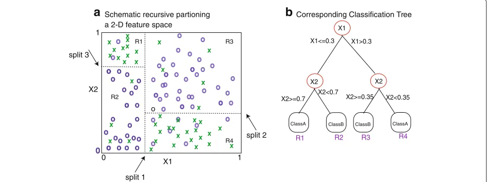
Random Forest is a machine learning technique that
leverages ensemble learning for classification. that relies on aggregates over bootstrapped CART model [4]. CART models have been widely used for decision making in several research areas, e.g., medicine, engineering, and marketing [3]. Their popularity is due in part to their natural interpretation and flexibility.
1) Input Data
2) Divide data into k-folds
3) Create Missing Data
4) Discretize
5) Application of Algorithms
CF
6) Evaluation of Performace Simulation Pipeline
RF/RFImpute RF/MI RF/kNN RF/MICE
LR/MI LR/kNN LR/MICE
0 20 40 60
RF_RFimpRF_MIRF_KNNRF_MIC E
LR_MI LR_kNNLR_MIC E
CF
Method
Misclassification Rate
Fig. 1The simulation pipeline proceeds in a series of steps: (1) The data is input, and (2) divided intoK-folds, (3) missing data is created at random, (4) the data is discretized, (5) a recommender system is fit along with variations of logistic regression and random forests, and the (6) performance is evaluated
training set can give rise to significantly different decision tree structures [19].
Random forests utilize CART models in an ensemble fashion to overcome instability and uncertainty in the population and predictor set. Therandomnesscomes in two ways that relate to resampling of the training data and the predictor set. Briefly, each model in the ensemble is based on a sample that is bootstrapped with replacement
from the training data. A decision tree is fit from the boot-strapped data. However, at each node in the tree, only a random subset ofmpredictors is considered for partition-ing, instead of the entire set. Empirically, RFs have been shown to be relatively insensitive over different values of
the new sample down each decision tree in the ensem-ble and aggregating over those predictions. Unfortunately, due to the aggregate nature of the ensemble, the natural interpretation of the CART model is not retained. Calcu-lations were performed in the R programming language using therandomForestpackage [4]. For dichotomous outcomes, the Brier score was calculated from the Out Of Bag (OOB) votes that arise from frequency prediction of classifications based on trees for which it was not in the bootstrap sample. Although this is not a probability, rather it is an OOB frequency of prediction, the Brier score is most often used for RF calibration [12].
Collaborative filtering is an algorithm that relies on user rating data for items to infer missing ratings for other users and items. This type of recommender system is widely used for the creation ofranked listsof items, that arepersonalizedin the sense that the inference is based on other users with similar patterns of ratings. Applica-tions to marketing are obvious. The scale of ratings is fixed across items. There are modifications to the standard CF that account foruser rating bias, which occurs when indi-viduals tend to always rate highly or poorly [28]. In certain applications this may be an issue, e.g., self-reporting, mea-surement, or doctor bias. The bias adjustment amounts to simply centering the rows (patients).
In the clinical application, users are patients, and items are derived from clinical features of the patients. Several of the measured features can be expected to be missing. We define the patients,P= {P1,P2,. . .Pn}, and the measured features on these patientsX = {X1,X2,. . .,Xp}. This cal-culation is performed on the ratings over a common set
of features, which have no missing values between the two patients. The similarity between patientsPiandPjis defined as the cosine distance between their features:
simcos(Pi(X), Pj(X)) = Pi(X),Pj(X) ||Pi(X)||||Pj(X)||
, (1)
where · denotes the inner product, and || · || is the euclidean norm.
FeatureXiof patientPjis estimated as:
ˆ
XiPj = 1
h∈N(Pj)simcos(Pj, h)
h∈N(Pj)
simcos(Pj, h)·Xh,i
(2)
whereh∈N(Pi)is the neighborhood centered on patient
Pi. A schematic depicting the notion of a neighborhood for a patientP9is shown in Fig. 2a. Missing data and out-come is predicted by aggregating across thekneighbors (Fig. 2b). Note that CF does not treat the clinical predic-tion problem as supervised, rather it recasts a supervised learning one as an unsupervised problem. In the execution of CF on clinical data, the response variableY is treated simply as another predictor,Xi, with the prediction being made as a function of patient similarity (Eq. 2).
In our applications, the selection of the number of neighbors, k, was made based on 3-fold cross val-idation. Implementation of CF was performed using recommenderlab in the R programming language (https://www.r-project.org). X1 X2 o o o o X o o o o o o o o o o o o o o o o o o o o o o o o o o o o o o o o o o o o o o o o o o o oo 0 split 1 split 2 split 3 1 1 0
a
Schematic recursive partioning a 2-D feature spaceR1 R2 R3 R4 o o o
o o o
o o X X X X X X X X X X X X X X X X X X X X X X X X X X X X X X X X X X X X X o o o o o o o o o o o o o o o o X X X X o o X1>0.3 X2<0.35
b
Corresponding Classification TreeR1 R2 R3 R4
ClassA X2>=0.35 X2<0.7 X1<=0.3 X2>=0.7 X1 X2 X2
ClassB ClassB ClassA
Simulation
Our objective is to assess the performance of CF based recommender systems comparatively to logistic regres-sion and random forests in clinical data with varying degrees of missingness. To this end, we have designed an experiment for manipulating the datasets to contain a percentage of missing values (NA). Each dataset was first examined atbaseline, which is the data withno additional missingness. For the NHANES and dermatology data this corresponds to 3 and 5% missing at baseline, respecitively. Chronic Kidney and SUPPORT 10 and 16% were missing at baseline, respectively. On top of the baseline missing-ness, a percentage of the data was deleted at random to mimic low (<16%), moderate (20%), and severe (30%), lev-els of missingness. Our simulation proceeds in six phases (Fig. 3). (1) The data is input, and (2) divided into 3−folds, (3) missing data is created at random, (4) the data is dis-cretized, (5) CF and classification models are fit, and the (6) performance is evaluated. Importantly, for each simu-lated setting steps 1–4 are performed, and the algorithms used for model fitting (step 5) utilizes same exact data in order to gain a fair assessment of their relative per-formance. We briefly detail each step in the simulation pipeline below.
1. Input data:The following datasets were input into
the simulation pipeline: Chronic Kidney,
Dermatology, NHANES, SUPPORT and simulated data.
2. Data divided into folds for cross-validation:Each
dataset is divided intoK=3folds for
cross-validation. The analyses were performed through 3-fold cross validation on each individual data set. Therefore, two thirds of the data were used as training data in each fold and the rest were used as test data. We utilize repeated cross-validation. In our applications to real data and simulation we repeat the cross validation process 50 times. For each run the
folds are fixed throughout the simulation of different levels of missingness to achieve a cumulative affect.
3. Creation of missing data:For the real datasets, a
fixed percentage of values in predictor variables were randomly deleted with the goal to simulate MCAR settings [22]. Since the deletion is random across all predictor variables, each is affected to a comparable extent. In all settings, the pattern of missing data is cumulative across the varying levels of severity. For example, for a given simulation, the missing values for the 20% simulation include, those missing in the 10% simulation. MAR was also imposed on the simulated
data by creating a dependency betweenX1onX2.
Specifically, missingness was imposed onX1ifX2
was above a specified quantile. The specified quantile was adjusted as to let in varying levels of missingness. MCAR was also used in connection with the
simulated data. The MCAR rate of missingness was matched to the MAR rate of missingness to enable fair comparisons. For each missing data scenerio, we simulated 50 unique patterns of missingness.
4. Discretization of continuous variables:
Recommender systems are designed to utilize ratings, which are categorical or ordinal values by nature. Moreover, the number of levels for each variable in the predictor set is fixed and uniform over the set of predictors. The datasets under consideration contain a mixture of variable types. Notably, RFs can readily accommodate a mixture of variable types in the predictor set. However, in order to facilitate fair comparisons, the predictor variables that have continuous values were discretized. Specifically, for each of the four data sets, the maximal levels taken by categorical or ordinal variables were used to
discretize continuous variables. For example, if data
setX has 2 categorical variables that have values
{1, 2}and{1, 2, 3}respectively, the continuous variables in this data set will be discretized into three
? ?
a
Local Neighborhood of size k=3b
Collaborative filtering for P9 on neighborhood of size k=3P9 P2 P3
P6
P1
P4
P5 P7
P8
levels and take on values{1, 2, 3}. The threshold for discretization of a continuous variable is based on
quantiles to ensure abalance between the
discretization levels. Following these principles, NHANES data were subject to 7-level discretization, while SUPPORT and Chronic Kidney Disease data were subject to 5-level discretizations, and
Dermatology data to 4-level discretization. Simulated data was also subject to 4-level discretization.
5. Application of algorithms for model fitting:CF
and classification methods were applied to each data set as described above. Briefly, different types of
imputation are described as follows: (1)Mean
imputation was used for each predictor variable in the training data. Imputation values were calculated as the average of the non-missing values within this predictor variable. Subsequently, this mean value replaced all of the missing values for the
corresponding variable. The mean value for the training data was also used for missing data in the
test set. (2)k-NN imputation was implemented
throughpreProcessandpredictfunctions in
thecaretpackage in R. The missing predictor variable values in training data and testing data were filled in through k-NN imputation respectively. Cross validation (3-fold) was used for the selection of k. (3) RF-Impute is an imputation within the
randomForestpackage in R. RF-impute begins with a median imputation, and the imputation is updated based on proximities after running an initial forest on the imputed data, see [5] for details. Missing values in testing data were imputed through mean imputation (as described above) instead of rf imputation. (4) Multivariate Imputation by Chained Equations (MICE) was applied using the R package
mice[7]. MICE uses Gibbs sampling to complete a
multivariate data set by iterating over a set of conditional densities representing the variabes in the dataset. Five datasets were imputed for each missing data setting.
6. Evaluation of Performance:Performance was based
on the mean misclassification rate (0−1loss) across
all the folds, and the standard error of this mean estimate was calculated as standard deviation across the folds.
Results
Baseline and simulated scenarios of low, moderate, and severe missing data were implemented for the chronic kid-ney, dermatology, NHANES, and SUPPORT datasets. For each simulation the data was divided into 3-folds, miss-ing data was created, discretization was performed. The following methods and imputations were evaluated: RF-RFImpute (RF Imp), RF with mean imputation (RF-MI),
RF with kNN imputation (RF-kNN), RF with MICE impu-tation (RF-MICE), LR with mean impuimpu-tation (LR-MI), LR with kNN imputation (LR-kNN), and LR with MICE (LR-MICE), and user-based CF. Performance was evalu-ated using the misclassification rate (Fig. 4), sensitivity (Table 1) and specificity (Table 2).
For the real data, every variation of LR and RFs out-performed recommender systems for every data set in each scenario of missing data (Fig. 4). The dermatology dataset was by far the worst performing, which has six classes in the response variable. MI proves to be espe-cially problematic for the dermatology data, espeespe-cially when the the level of missingness increases (Fig. 4c–d). For the large datasets (NHANES and SUPPORT) MI, kNN and MICE imputation led to only marginal differences in the misclassification rate when the level of missingness is low-moderate (Fig. 4a–b). The advantages if MICE can be observed when the level of missingness is more severe (Fig. 4b–c).
LR offers clear advantages over RF for the dermatology data. Otherwise, the performance of LR and RF is com-parable, especially when used in connection with MICE (Fig. 4c-d). The HL test indicates good calibration of LR models (P-value> 0.05) (Additional file 1: Table S5). The HL test generally revealed improved calibration with increasing missingness. This was observed with NHANES for MI, kNN, and MICE, and with SUPPORT using MICE (Additional file 1: Table S5). This is not surprising, espe-cially given the conditional nature of the imputation for MICE, but is potentially misleading as it may not reflect the underlying population well. The Brier score for RF and LR notably small, which also supports good calibration (Additional file 1: Table S6). The improving nature of the fit as a function of missingness was not observed in the Brier score as it was with the HL test.
For datasets with a dichotomous response, the sensitiv-ity and specificsensitiv-ity was calculated for CF, along with LR and RF for imputation methods, MI and MICE (Tables 1 and 2). Both the sensitivity and specificity of CF is often inferior for CF, with the exception of the sensitivity of the Kidney data with low-moderate levels of missingness (Tables 1 and 2). Generally, there is not a major differ-ence or trend between in sensitivity or specificity that differentiates LR and RF for a given imputation method.
RF_RFImp RF_MI
RF_kNN RF_MICE LR_MI LR_kNN LR_MICE CF
RF_RFImp RF_M
I
RF_kNN RF_MIC
E
LR_MI
LR_kNN LR_MICE
CF
RF_RFImp RF_MI
RF_kNN RF_MIC
E
LR_M I
LR_kNN LR_MICE
CF
RF_RFImp RF_M
I
RF_kNN RF_MIC
E
LR_MI
LR_kNN LR_MICE
CF
Dermatology (5% missing - baseline)
NHANES (3% missing -baseline) Chronic Kidney (10% missing - baseline) Dermatology (10% missing)
NHANES (10% missing)
SUPPORT (16% missing - baseline)
Chronic Kidney Dermatology
NHANES SUPPORT
Chronic Kidney Dermatology
NHANES SUPPORT
0 0.2 0.4 0.6
0 0.2 0.4 0.6
0 0.2 0.4 0.6
0 0.2 0.4 0.6
a
>10% Missingb
10-16% Missingc
20% Missingd
30% MissingMisclassification Rate
Misclassification Rate
Misclassification Rate
Misclassification Rate
Fig. 4Simulation results for Chronic Kidney, Dermatology, NHANES, and SUPPORT are shown foraless than 10% missing data,b10–16% missing data,c20% missing data,d30% missing data. Graphs depict the mean estimate of misclassification and standard error calculated via repeated 3-fold cross validation for 50 simulated patterns of missingness for each level of severity. The results for the baseline levels of missingness for each data sets is captured inaandb
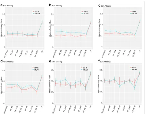
RF or LR (Fig. 5e, f). In more severe settings, MICE was also the superior imputation method for both MAR and MCAR (Fig. 5d, e and f). MAR and MCAR patterns of missingness of the same type were also simulated on data with class imbalance. The overall results are consistent with the real data and balanced simulations. Traditional classification methods outperform CF in every setting (Additional file 1: Figure S1). The differences in perfor-mance between CF and traditional classification methods are much more pronounced in the severe imbalanced set-tings for both MAR and MCAR (Additional file 1: Figure S1G-I). Notably, for the traditional classification methods,
the degree of imbalance had a lesser impact on perfor-mance compared to the level of missingness. In fact, with low levels of missingness (Additional file 1: Figure S1 A, D, G) MAR and MCAR are almost indistinguish-able, although performance degrades slightly. Whereas, high class imbalance leads to more variability between methods (Additional file 1: Figure S1 C, F, I).
Discussion
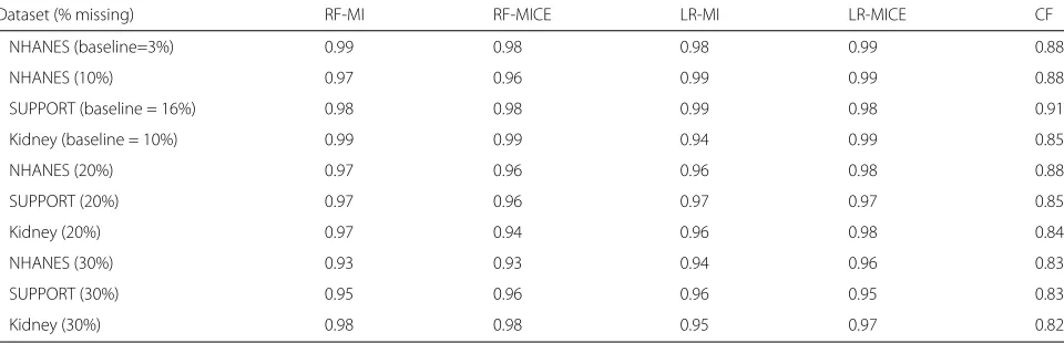
Table 1Sensitivity for the most competitive classifiers and imputation combinations and CF
Dataset (% missing) RF-MI RF-MICE LR-MI LR-MICE CF
NHANES (baseline=3%) 0.99 0.99 0.99 0.99 0.56
NHANES (10%) 0.98 0.99 0.98 0.99 0.63
SUPPORT (baseline = 16%) 0.99 0.98 0.98 0.97 0.98
Kidney (baseline =10%) 0.99 0.98 0.97 0.99 0.99
NHANES (20%) 0.98 0.98 0.99 0.99 0.49
SUPPORT (20%) 0.96 0.96 0.84 0.98 0.86
Kidney (20%) 0.98 0.99 0.98 0.98 0.98
NHANES (30%) 0.89 0.99 0.89 0.95 0.25
SUPPORT (30%) 0.86 0.99 0.81 0.93 0.82
Kidney (30%) 0.98 0.98 0.97 0.96 0.92
prediction of adverse outcomes following a heart attack [21]. In this context, they demonstrated superior results (although slight) to competing statistical and machine learning methods for risk prediction. These comparisons were made to logistic regression models and support vector machines. The data inherently contained miss-ing values, as was the case for the data in the present study, but additional missing data was notpushed in to the study and the focus was on a single dataset that is not publicly available. Our study has arrived at different conclusions regarding superiority of CF to classification methods. However, the overall study design and datasets are fundamentally different, and should be viewed as complimentary (not contradictory) to the work of Hassan et al.
At present, we are in the “Big Data” era, and it is becom-ing commonplace to reach for methods like CF, that are frequently used in other disciplines, to solve challenging problems in biomedical research. To this end, we antic-ipate more activity and attraction to this area. However, there remain many open questions regarding the utility of recommender systems on biomedical data for the purpose of clinical prediction, or more generally, classification. The
study by Hassan et al. represents a novel framework for prediction of this type and has motivated further research in this direction [32, 34]. Their study, and ours, is limited in terms of size and uses cohorts from population studies or clinical trials. In our case, this was due to the lack of accessibility to medical databases, which are generally not publicly available.
The study by Hassan et al., and the present study, are fundamentally different to other research in the area that has centered on CF for comorbidity prediction on dis-eased codes [9, 17, 18]. It is natural to consider combining disease codes with additional attributes such as clinical data, patient history, and demographics to improve pre-diction. Data integration is a major challenge for “Big Data” and the translation of data to knowledge [26]. Although the present study is of small scale, we demon-strate the clinical data that can be modeled using tra-ditional classification methods is preferable to CF. This study may be informative to developing and understand-ing approaches to data integration on a large-scale. On the other hand, there are several situations that may be inher-ent to a “Big Data” application that would prohibit the use of traditional classification methods. For example, the
Table 2Specificity for the most competitive classifiers and imputation combinations and CF
Dataset (% missing) RF-MI RF-MICE LR-MI LR-MICE CF
NHANES (baseline=3%) 0.99 0.98 0.98 0.99 0.88
NHANES (10%) 0.97 0.96 0.99 0.99 0.88
SUPPORT (baseline = 16%) 0.98 0.98 0.99 0.98 0.91
Kidney (baseline = 10%) 0.99 0.99 0.94 0.99 0.85
NHANES (20%) 0.97 0.96 0.96 0.98 0.88
SUPPORT (20%) 0.97 0.96 0.97 0.97 0.85
Kidney (20%) 0.97 0.94 0.96 0.98 0.84
NHANES (30%) 0.93 0.93 0.94 0.96 0.83
SUPPORT (30%) 0.95 0.96 0.96 0.95 0.83
MA R MCAR MA R
MCAR MA R
MCAR
MA R MCAR MA R
MCAR MA R MCAR MA R
MCAR
MA R MCAR
0 0.1 0.2 0.3
0 0.1 0.2 0.3
0 0.1 0.2 0.3 0 0.1 0.2 0.3
0 0.1 0.2 0.3
0 0.1 0.2 0.3
a
10% Missingb
20% Missingc
30% Missingd
40% Missinge
50% Missingf
60% MissingRF_RFImp RF_M
I
RF_kNN RF_MICE LR_M I
LR_kNN LR_MICE CF
RF_RFImp RF_M
I
RF_kNN RF_MICE LR_MI LR_kNN LR_MICE CF
RF_RFImp RF_M
I
RF_kNN RF_MIC E
LR_M I
LR_kNN LR_MICE CF
RF_RFImp RF_M
I
RF_kNN RF_MICE LR_M I
LR_kNN LR_MICE CF
RF_RFImp RF_M
I
RF_kNN RF_MIC E
LR_M I
LR_kNN LR_MICE CF
RF_RFImp RF_MI
RF_kNN RF_MIC E
LR_M I
LR_kNN LR_MICE CF
Misclassification Rate
Misclassification Rate
Misclassification Rate
Misclassification Rate
Misclassification Rate
Misclassification Rate
Fig. 5Results for simulated data under MAR and MCAR fora10% missing data,b20% missing data,c30% missing ,d40% missing data,e50% missing data andf60% missing data. Graphs depict the mean estimate of misclassification and standard error calculated via repeated 3-fold cross validation for 50 simulated patterns of missingness for each level of severity
fusion of databases that have unified data representation, or the use ofreal timepredictions that do not require re-training or tuning of the database, but rather merge new patient data in a seamless manner.
The present study was motivated by a desire to develop a more comprehensive understanding as to (1) how rec-ommender systems perform on medical data, and (2) how this performance changes with an increased num-ber of missing values. To address these questions, we set out to examine CF in a variety of controlled (simu-late missing data) yet realistic (medical data sets) settings. We examined four different publicly available data sets, NHANES, SUPPORT, Chronic Kidney, and Dermatology. These datasets differed in both scope and size, but each had an outcome and could be framed as a classification problem.
Our simulation pipeline involved division into folds, creation of missing data, discretization, application of
learning repository [16]. RF is an attractive competitor for this study because of the ensemble nature, ability to handle missing data, and it is generally robust to noise and outliers [4]. Moreover, variations of the RF approach have been shown to be effective in “Big Data” settings, such as electronic health records [27]. Had recommender systems not been consistently inferior, a deeper investiga-tion of alternative classificainvestiga-tion methods would have been warranted.
Another limitation of our study is the amount and pat-tern of missing data. Limitations on the amount of missing data were largely a function of the CF implementation in recommenderlab, where 30% was the maximum that could be achieved without errors related to the identi-fication of k nearest neighbors (even for small k). The
missingness of the data was simulated as missing com-pletely at random. In realistic settings, this may not be the case, especially in databases housing electronic health records. However, the simulation of not missing at ran-domis notably more difficult and subject to intense bias. Finally, a discretization of the data is required for recom-mender systems. Our approach to discretization was to have it dictated by the number of levels in non-continuous variables, and assigning the data according to quantiles. However, recommender systems often work on a likert scale and are ordinal in nature. We found this makes the discretization process rather awkward for medical data. In general, the discretization process results in a substan-tial amount of information loss. To this end, LR models and RFs are inherently flexible in that mixed predic-tors (continuous, categorical, etc.) can be accommodated. However, in order to level the playing field and facilitate the most fair comparisons, we discretized (unnecessarily) the continuous predictors. Application of classifiers to the original (non-discretized) data would have led to improve-ments in performance, and consequently widened the gap between CF and traditional classification methods. The relative size of the classes for the response variable also influences performance, especially in situations of severe imbalance. Our simulations showed that CF was particu-larly sensitive to class imbalance (Additional file 1: Figure S1). One possibility for this is the discretization will be negatively impacted. In our simulated data, we also dis-cretized continuous variable for traditional classification methods. However, for CF, we hypothesize that the dis-cretization has more of an impact on the model due to the nature of the the class assignment and the depen-dency on similarities (Eq. 1–2). The clinical data that we considered was relatively well balanced, with most severe imbalance for NHANES (35% minority class rate). Since imposing class imbalance on the real data would require subsetting or resampling the data, and consequently cut-ting down the sample size, we examined the impact of class imbalance on simulated data with missingness that
is MAR or MCAR. Therefore, CF did not appear to offer any obvious advantage in these settings, but teasing out the contributions of the imbalance and the missingness in a real clinical data set would prove to be more challenging, and will be an area of future research. Notably, RFs have shown promise in class imbalance problems via down sampling and weighted loss [10], and we hypothesize that they would be generally more effective in imbalanced settings.
The size of the feature space is a major consideration. If the feature space is high-dimensional (N << p) there are many conceptual issues that arise with the concept of nearest neighbor that are rooted in the inherent sparsity of the feature space [19, 23]. The proximity of a neigh-bor increases considerably as the size of feature space increases. The local nature of k-NN calls into question the value and quality of a neighbor [19]. In the context of a rich marketing database, issues related to the dimen-sion of the feature space issue are often secondary to the extreme sparsity of the data. However, in the case of med-ical data, the issue of poor neighbor quality may not only arise, but may also be masked by the discretization pro-cess. This would certainly be the case in the classic “Big Data” settings, where the population itself is severely het-erogenous. These weaknesses for large, sparse databases are also recognized in more classical, non-medical applications [20, 30].
Lack of stability and quality of the neighbor is also reflected in the implementation of RFs with kNN impu-tation with severe missing data for dermatology (Fig. 4d). On the other hand, CF did not exhibit this instabil-ity, although the performance was uniformly poor. The underlying models for kNN imputation in a RF and CF based recommender systems are essentially identical in how the predictor set is imputed. The difference lies in how the response is handled. The problem is treated as a supervised one for kNN imputation in a RF, and unsu-pervised for CF based recommender systems. Generally, re-casting problems that are unsupervised as supervised is a populartrickin data mining, as there are several advan-tages due to the fact that there is an outcome, andlosscan be measured [19]. On the contrary, casting a problem that is supervised as unsupervised, as in this approach, does not offer the same advantages.
quality of neighborissue would still remain for alternative similarities and methods. Therefore, we hypothesize that datasets modeled using traditional classification methods will likely achieve better performance when compared to CF-based methods.
Conclusions
In summary, our results consistently put CF in a poor light for clinical prediction. We observed overwhelming evi-dence that traditional classification methods outperform user based-CF in simulation and real clinical datasets, across different levels of missing data mechanisms of missingness, as well as class imbalance in the response variable. The results of this work call into question CF as a general strategy for risk prediction in datasets where classification is an acceptable alternative [21, 32, 34]. In this setting, recasting a supervised learning problem as unsupervised was demonstrated to be suboptimal. This is not to say that CF does not, and will not, have utility for medical data. Scalability, dynamic learning, and merg-ing of database are practical challenges that make CF an attractive option. However, we strongly suggest exercising caution if the objective is classification, and the size of the data can be accommodated with traditional classification methods or alternative machine learning approaches.
Additional file
Additional file 1:Contains Supplemental Figure 1 and Supplemental Tables 1–6.
Abbreviations
CART: Classification and regression tree; kNN: k-nearest neighbors; LR: Logistic regression; LR- MI: Logistic regression with MICE imputation; LR- MICE: Logistic regression with MICE imputation; MAR: Missing at random; MCAR: Missing completely at random; MI: Mean imputation; MICE: Multivariate imputation by Chained equations; MNAR: Missing not at random; NHANES: National health and nutrition examination survey; RecSys: Recommender systems; RF: Random forest; RF-kNN: Random forest with k-nearest neighbor imputation; RF-MI: Random forest with mean imputation; RF- MICE: Random forest with MICE imputation; RF- RFImp: Random forest with random forest imputation; SUPPORT: Study to understand prognoses preferences outcomes and risks of treatment
Acknowledgements Not applicable.
Funding
RHB was supported through NSF DMS 1557593 and NSF DMS 1312250.
Availability of data and materials
The data utilized in this study is secondary data that was obtained from publicly available sites (see Materials and Methods). The NHANES data is available through the site (http://wwwn.cdc.gov/nchs/nhanes/). The SUPPORT study is available through the collection provided by the Department of Biostatistics at Vanderbilt University [15]. Chronic kidney disease data and the dermatology data was obtained through the UCI machine learning repository (http://archive.ics.uci.edu/ml/) [1].
Authors’ contributions
RHB conceived and designed the study. RHB and FH performed the analysis. RHB and FH wrote the manuscript, and both agree to be accountable for all aspects of the study. Both authors read and approved the final manuscript.
Competing interests
The authors declare that they have no competing interests.
Consent for publication Not applicable.
Ethics approval and consent to participate Not applicable.
Received: 6 May 2016 Accepted: 7 November 2016
References
1. Asuncion A, Newman DJ. UCI Machine Learning Repository.School of
Information and Computer Science. Irvine: University of California; 2007. http://www.ics.uci.edu/~mlearn/MLRepository.html.
2. Breese JS, Heckerman D, Kadie C. Empirical analysis of predictive
algorithms for collaborative filtering. In: Proceedings of the Fourteenth conference on Uncertainty in artificial intelligence. Burlington: Morgan Kaufmann Publishers Inc.; 1998.
3. Breiman L, Friedman J, Stone CJ, Olshen RA. Classification and
regression trees. Boca Raton: CRC press; 1984.
4. Breiman L. Random forests. Mach Learn. 2001;45(1):5–32.
5. Breiman L. Random forests. Mach learn. 2001;45.1:5–32.
6. Brody DJ, et al. Blood lead levels in the US population: phase 1 of the
Third National Health and Nutrition Examination Survey (NHANES III, 1988 to 1991). Jama. 1994;272.4:277–83.
7. Buuren S, Groothuis-Oudshoorn K. mice: Multivariate imputation by
chained equations in r. J Stat Softw. 2011;45.3:. doi:10.18637/jss.v045.i03.
8. Castelluccio M. The music genome project. Strat Financ. 2006;88(6):57.
9. Chawla NV, Davis DA. Bringing big data to personalized healthcare: a
patient-centered framework. J Gen Intern Med. 2013;28(3):660–5. 10. Chen C, Liaw A, Breiman L. Using random forest to learn imbalanced
data. Berkeley: University of California; 2004, pp. 1–12.
11. Connors AF, Dawson NV, Desbiens NA, Fulkerson WJ, Goldman L, Knaus WA, Lynn J, Oye RK, Bergner M, Damiano A, et al. A controlled trial to improve care for seriously iii hospitalized patients: The study to understand prognoses and preferences for outcomes and risks of treatments (support). JAMA. 1995;274(20):1591–8.
12. Dankowski T, Ziegler A. Calibrating random forests for probability estimation. Stat Med. 2016.
13. Davis DA, Chawla NV, Blumm N, Christakis N, Barabási AL. Predicting individual disease risk based on medical history. In: Proceedings of the 17th ACM conference on Information and knowledge management. New York: ACM; 2008. p. 769–78.
14. Davis DA, Chawla NV, Christakis NA, Barabási A-L. Time to care: a collaborative engine for practical disease prediction. Data Min Knowl Disc. 2010;20(3):388–415.
15. Department of Biostatistics Vanderbilt University. Data collecton. 2015. http://biostat.mc.vanderbilt.edu/DataSets.
16. Fernández-Delgado M, Cernadas E, Barro S, Amorim D. Do we need hundreds of classifiers to solve real world classification problems. J Mach Learn Res. 2014;15(1):3133–81.
17. Folino F, Pizzuti C. A recommendation engine for disease prediction. IseB. 2015;13(4):609–28.
18. Folino F, Pizzuti C, Ventura M. A comorbidity network approach to
predict disease risk.Information Technology in Bio-and Medical Informatics,
ITBAM 2010. Berlin: Springer; 2010, pp. 102–9.
19. Friedman J, Hastie T, Tibshirani R. The elements of statistical learning, volume 1. Springer series in statistics Springer. Berlin; 2001.
20. Good N, Schafer JB, Konstan JA, Borchers A, Sarwar B, Herlocker J, Riedl J. Combining collaborative filtering with personal agents for better recommendations. In: AAAI/IAAI. Palo Alto: Association for the Advancement of Artificial Intelligence (AAAI); 1999. p. 439–46. 21. Hassan S, Syed Z. From netflix to heart attacks: collaborative filtering in
22. Heitjan DF, Basu S. Distinguishing ?missing at random? and ?missing completely at random? Am Stat. 1996;50(3):207–13.
23. Hinneburg A, Aggarwal CC, Keim DA. What is the nearest neighbor in high dimensional spaces? In: 26th Internat. Conference on Very Large Databases. New York: ACM; 2000. p. 506–15.
24. Hosmer DW, Lemesbow S. Goodness of fit tests for the multiple logistic regression model. Commun Stat Theory Methods. 1980;9(10):1043–69. 25. Jr Hosmer DW, Lemeshow S. Applied logistic regression. Hoboken: John
Wiley & Sons; 2004.
26. Margolis R, Derr L, Dunn M, Huerta M, Larkin J, Sheehan J, Guyer M, Green ED. The National Institutes of Health’s big data to knowledge (BD2K) initiative: capitalizing on biomedical big data. J Am Med Inform Assoc. 2014;21(6):957–8.
27. Mathias JS, Agrawal A, Feinglass J, Cooper AJ, Baker DW, Choudhary A. Development of a 5 year life expectancy index in older adults using predictive mining of electronic health record data. J Am Med Inform Assoc. 2013;20(e1):e118–e124.
28. Ricci F, Rokach L, Shapira B. Introduction to recommender systems handbook. Berlin: Springer; 2011.
29. Rubin DB. Inference and missing data. Biometrika. 1976;63(3):581–92. 30. Sarwar BM, Konstan JA, Borchers A, Herlocker J, Miller B, Riedl J. Using
filtering agents to improve prediction quality in the grouplens research collaborative filtering system. In: Proceedings of the 1998 ACM conference on Computer supported cooperative work. New York: ACM; 1998. p. 345–54.
31. Scirica BM, Morrow DA, Hod H, Murphy SA, Belardinelli L, Hedgepeth CM, Molhoek P, Verheugt FWA, Gersh BJ, McCabe CH, et al. Effect of ranolazine, an antianginal agent with novel electrophysiological properties, on the incidence of arrhythmias in patients with non–st-segment–elevation acute coronary syndrome results from the metabolic efficiency with ranolazine for less ischemia in non–st-elevation acute coronary syndrome–thrombolysis in myocardial infarction 36 (MERLIN-TIMI 36) randomized controlled trial. Circulation. 2007;116(15): 1647–52.
32. Sodsee S, Komkhao M. Evidence-based medical recommender systems: A review. Int J Inf Process Manag. 2013;4(6):114–20.
33. Steyerberg EW, Vickers AJ, Cook NR, Gerds T, Gonen M, Obuchowski N, Pencina MJ, Kattan MW. Assessing the performance of prediction models: a framework for some traditional and novel measures. Epidemiol (Cambridge, Mass.) 2010;21(1):128.
34. Yao J, Azam N. Web-based medical decision support systems for three-way medical decision making with game-theoretic rough sets. IEEE Trans Fuzzy Syst. 2015;23(1):3–15.
• We accept pre-submission inquiries
• Our selector tool helps you to find the most relevant journal
• We provide round the clock customer support
• Convenient online submission
• Thorough peer review
• Inclusion in PubMed and all major indexing services
• Maximum visibility for your research
Submit your manuscript at www.biomedcentral.com/submit