A P-value model for theoretical power analysis and its applications in multiple testing procedures

R E S E A R C H A R T I C L E

Open Access

A

P-value model for theoretical power

analysis and its applications in multiple testing

procedures

Fengqing Zhang

and Jiangtao Gou

Abstract

Background: Power analysis is a critical aspect of the design of experiments to detect an effect of a given size. When multiple hypotheses are tested simultaneously, multiplicity adjustments top-values should be taken into account in power analysis. There are a limited number of studies on power analysis in multiple testing procedures. For some methods, the theoretical analysis is difficult and extensive numerical simulations are often needed, while other methods oversimplify the information under the alternative hypothesis. To this end, this paper aims to develop a new statistical model for power analysis in multiple testing procedures.

Methods: We propose a step-function-basedp-value model under the alternative hypothesis, which is simple enough to perform power analysis without simulations, but not too simple to lose the information from the alternative hypothesis. The first step is to transform distributions of different test statistics (e.g.,t, chi-square orF) to distributions of correspondingp-values. We then use a step function to approximate each of thep-value’s distributions by matching the mean and variance. Lastly, the step-function-basedp-value model can be used for theoretical power analysis. Results: The proposed model is applied to problems in multiple testing procedures. We first show how the most powerful critical constants can be chosen using the step-function-basedp-value model. Our model is then applied to the field of multiple testing procedures to explain the assumption of monotonicity of the critical constants. Lastly, we apply our model to a behavioral weight loss and maintenance study to select the optimal critical constants.

Conclusions: The proposed model is easy to implement and preserves the information from the alternative hypothesis.

Keywords: Critical constants, Multiple testing procedures, Power analysis,p-value

Background

Power analysis is a key technique in the experimental design to reveal an effect of a given size. Traditional power calculation usually assumes a single hypothesis test, but it is quite common for researchers to test several hypothe-ses simultaneously. Clinical trials often require two or more hypotheses to be tested, and studies which involve comparing treatments using multiple outcome measures happen frequently in medical research [8]. The devel-opment of high-throughput biology leads to a dramatic increase in the number of hypothesis tests in genomics

*Correspondence: [email protected]

1_{Department of Psychology, Drexel University, 3201 Chestnut Street, 19104} Philadelphia, USA

Full list of author information is available at the end of the article

[20]. However, there are a limited number of studies on power analysis in multiple testing procedures. For scien-tific studies with multiple hypotheses, in order to correctly control the false positives, multiplicity adjustments to p-values should be taken into account in power anal-ysis. A consequence of multiplicity adjustments is the loss of power [21] and the change in sample size requirements [16].

Thep-value is a tail probability given the null hypothesis is true. Under the null hypothesis, thep-value is a uni-formly distributed random variable between 0 and 1. If the null hypothesis is false, thep-value’s distribution depends

on the alternative hypothesis, which usually satisfies the inequality

Pr(P≤p)≥p, (1)

i.e., the random variablePis less than a standard uniform random variable in the stochastic order, where the random variablePis the probability of rejecting the null hypothesis when the alternative hypothesis is true.

In order to perform a p-value based power analysis, certain distribution models are needed to describe the behavior ofp-values under the alternative hypothesis. In general there are two approaches. The p-value models based on the original test statistics [17] or based on copu-las [27] are usually with complex expressions, and further calculations or evaluations require integrations. So the theoretical analysis is difficult and numerical simulations are often needed. The p-value models based on Dirac function [10, 24] are over-simplified, which limits their application areas.

In this paper, we propose the step-function-based p-value models under the alternative hypothesis, which are simple enough to perform theoretical power analysis, but not too simple to lose the information from the alter-native hypothesis. Two applications in multiple testing procedures are shown and one application in weight-loss treatment is given.

Methods

A widely used p-value model assumes that the statis-tic under the null hypothesis follows N(0, 12_{), and}

the statistics under the alternative hypothesis follows N(δ, 12_{). Thep-values are calculated based on one-sided}

test [17].

The density function of the normal-distribution-based p-value model is

h(p)= φ

−1_(p)+δ

φ−1_(p) , (2)

with mean and variance

E[P]=

_+∞

−∞ (x)φ (x+δ)dx,

var[P]=

_+∞

−∞ [(x)]

2_{φ (x+δ)dx}

− +∞

−∞ (x)φ (x+δ)dx

2

.

Alternatively, we propose a step-function-basedp-value model under the alternative hypothesis, which has a den-sity function

h(p)=

⎧ ⎪ ⎪ ⎨ ⎪ ⎪ ⎩

f, 0≤p≤ 1−g f −g, g, 1−g

f −g <p≤1,

(3)

with mean and variance

E[P]= 1−2g+fg

2f −g , var[P]=

1+4fg2+4f2g−3f2g2 12f −g2 , where 0 ≤ g ≤ 1 ≤ f. The parameter(f,g) indicates the deviation of the random variable P under the step-function-based p-value model from a standard uniform random variable.

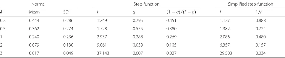
For comparison between the normal-distribution-based p-value model and the step-function-based p-value model, the parameters (f,g) of the step-function-based p-value model were chosen to match the means and the variances for the normal-distribution-based p-value model with parameterδ, as shown in Table 1. For the sim-plified step-function-basedp-value model with parameter f, means are matched with the normal model.

In addition, a simplified step-function-based p-value model with a single parameter f ∈[ 1,+∞) is achieved when assumingg = 0. The corresponding density func-tion is

h0(p)=

⎧ ⎪ ⎪ ⎨ ⎪ ⎪ ⎩

f, 0≤p≤ 1 f,

0, 1

f <p≤1.

(4)

with mean and variance

E[P]= 1

2f, var[P]= 1 12f2.

For the simplified step-function-based p-value model, a larger parameterf corresponds to a larger effect size. As a

Table 1Normal-distribution-basedp-value model and step-function-basedp-value model

Normal Step-function Simplified step-function

δ Mean SD f g (1−g)/(f−g) f 1/f

0.2 0.444 0.286 1.249 0.795 0.451 1.127 0.888

0.5 0.362 0.274 1.728 0.555 0.380 1.382 0.724

1 0.240 0.236 2.937 0.288 0.269 2.086 0.480

2 0.079 0.130 9.061 0.059 0.105 6.357 0.157

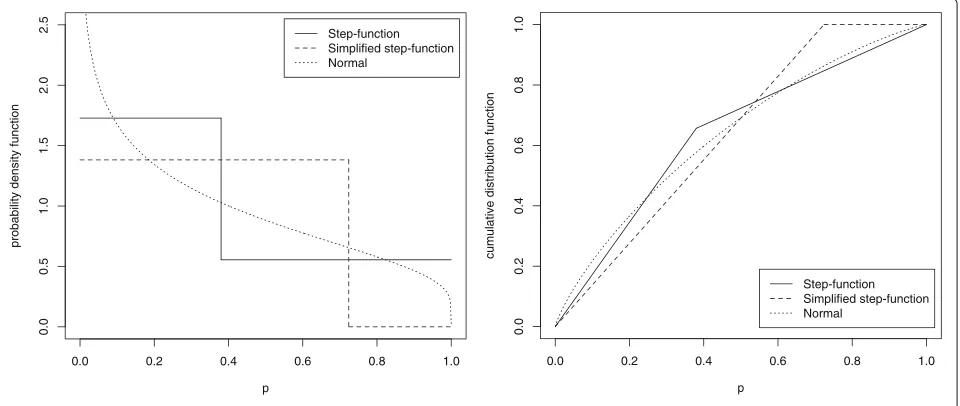
special case, whenf =1, the distribution is uniform [ 0, 1]. The probability density functions and the cumulative dis-tribution functions of the normal-disdis-tribution-based and the step-function-basedp-value models are compared in Fig. 1. The step-function-basedp-value models serve an approximation to thep-value models based on the original test statistics.

Based on the univariate model, the corresponding mul-tivariatep-value model has a density function

h(p1,· · ·,pn)= n

i=1

hi(pi), (5)

where differenthi(·)’s may have different parametersfi’s

and gi’s. In the following sections, the simplified

step-function-basedp-value model is applied to two problems in multiple testing procedures.

Results

Application: optimal choices of the critical constants

Assumenhypotheses{Hi}ni=1withp-values

pi

n i=1. Sort

p-values as p(1) ≤ · · · ≤ p(n), and H(1),· · ·,H(n) are

the corresponding null hypotheses. Consider testing the global null hypothesis∩n_i=1Hiunder the control of type I

error [15]

Pr∪n_i=1p(n−i+1)≤ciα

≤α.

The global test comparesp₍n−i+1)with its

correspond-ing critical constant ciα for every i = 1,· · ·,n. If for

some i’s, p(n−i+1) ≤ ciα, then the global null

hypoth-esis is rejected. Simes [25] proposed a test with ci =

(n−i+1) /n, and other choices ofci’s were proposed by

Rom [22], Cai and Sarkar [7], Gou and Tamhane [11].

Among different choices of critical constantsci’s,

peo-ple usually run simulations [19] or rely on numerical calculations [14] to make power comparison in order to choose suitable sets of critical constants. Besides the existing computationally intensive methods, the step-function-basedp-value model is an alternative choice to theoretically calculate the powers and make comparisons between different multiple testing procedures.

In this section we first show how the most powerful crit-ical constants can be chosen using our proposed method for a global test with two hypotheses, and then we can apply the successive recursion process to calculate the power for a global test withn hypotheses. For a global test with two single hypotheses, the control of type I error under independence requires

Prp(2)≤c1α

∪p(1)≤c2α

=α, wherec1≥c2. This equality is equivalent to

(1−2c2)+c1(2c2−c1) α=0. (6)

From (6) we getc2= 1−c

2 1α

2(1−c1α), and the derivative

dc2

dc1 =

−(c1−c2)α

1−c1α , which is less than zero. Soc2decreases whenc1 increases.

By using the simplified step-function-based p-value model, without loss of generality, we assume 1 ≤f1≤f2,

the probability of rejecting the global hypothesis is

Rejection probability

= ⎧ ⎪ ⎨ ⎪ ⎩

c2

f1+f2

α+c1(c1−2c2)f1f2α2, whenf1≤f2≤_c11_α,

c1f1+c2f2

α−c1c2f1f2α2, whenf1≤c11α≤f2≤c21α,

1, whenf1≥c11αorf2≥c21α.

When the global hypothesis contains two single hypotheses (n = 2), there are two configurations of

0.0 0.2 0.4 0.6 0.8 1.0

0.0

0.5

1.0

1.5

2.0

2.5

p

probability density function

Step-function Simplified step-function Normal

0.0 0.2 0.4 0.6 0.8 1.0

0.0

0.2

0.4

0.6

0.8

1.0

p

cumulative distribution function

Step-function Simplified step-function Normal

true and non-true null hypotheses where the global null hypothesis is false: (1) one true null hypothesis (n0 = 1)

and one false null hypothesis (m = 1), and (2) two false null hypotheses (m=2).

First, assume that one null hypothesis is true and the other is false, say,f1=1 andf2=f, then the power is

Power= ⎧ ⎪ ⎨ ⎪ ⎩ c2

1+fα+fc1(c1−2c2) α2 whenf ≤c1α1 ,

c1+fc2

α−fc1c2α2, when _c1α1 ≤f ≤ _c2α1 ,

1, whenf ≥_c2α1 .

Whenf ≤ _c1

1α, from (6) it follows thatc1(c1−2c2) α = 1−2c2, therefore

c2

1+fα+fc1(c1−2c2) α2=

f −f −1c2

α,

hence power increases whenc2decreases (c1increases).

When _c1

1α ≤ f ≤

1

c2α, from (6) we get c1c2α =

1 2

2c2−1+c21α

, consequently

c1+fc2

α−fc1c2α2= α

2

f+2c1−fαc21

= 1

2f

1+f2α−fαc1−1

2

.

Note that fαc1 ≥ 1, so power increases when c1

decreases (c2increases).

We calculate the maximal power for different f’s. When we assume the alternative hypothesis has a small effect size, where f ≤ 1/√α, the maximal power is achieved when c2 = 0 and c1 = 1/√α. When we

assume the alternative hypothesis has a moderate effect size, where 1/√α < f ≤ 1+√1−α/α, the max-imal power is achieved when c1 = 1/

fα and c2 =

f2α−1/2αff −1, so whenf increases, we can fol-low the strategy to decreasec1(increasec2) to achieve the

maximal power. When we assume the alternative hypoth-esis has a large effect size, wheref >1+√1−α/α, the maximal power is achieved when we choose a test with c2 ≥ 1/

fα, so whenf is large enough, different tests have similar power.

max Power= ⎧ ⎪ ⎪ ⎨ ⎪ ⎪ ⎩

fα, whenf ≤√1

α,

1+f2α

2f , when √1α <f ≤ 1+ √

1−α

α ,

1, whenf > 1+ √

1−α

α .

(7)

Second, assume that both null hypothesis are false with the same effect size, say,f1=f2=f, then the power is

Power=

2fc2α+f2c1(c1−2c2) α2, whenf ≤ _c1α1 ,

1, whenf ≥ _c1α1 .

Whenf ≤ _c1

1α, from (6) we getc1(c1−2c2) α=1−2c2, then

2fc2α+f2c1(c1−2c2) α2=fα

f −2f −1c2

,

power increases whenc2decreases (c1increases).

We calculate the maximal power for differentf values. When we assume both hypotheses are false and with a small effect size, wheref ≤1/√α, the maximal power is achieved whenc2= 0 andc1=1/√α. When we assume

both false hypotheses have a big effect size, where f ≥ 1/√α, the maximal power is achieved when the test satis-fiesc1≥1/

fα. By taking bothf ≤1/√αandf ≥1/√α into account, it follows thatc1= 1/√αandc2= 0 is the

uniformly best choice when both null hypotheses are false.

max Power=

f2α, whenf ≤ √1 α,

1, whenf > √1 α.

(8)

In general, for a global test with n single hypothe-ses, where m of them are true significances (false null hypotheses), define the probabilities as

Bn,m,i

= ⎧ ⎪ ⎪ ⎨ ⎪ ⎪ ⎩

Prn,mp₍n)≤c1α

, i=1,

Prn,mp₍n)>c1α,· · ·,p(n−i+2)>ci−1α,p(n−i+1)≤ciα, i=2,· · ·,n, Prn,mp₍n)>c1α,· · ·,p₍1)>cnα, i=n+1,

where Prn,m indicates the probability for n hypotheses,

wheremis the number of the true significances, andn0=

n−mis the number of the true nulls. Since

Bn,m,n=Prn,m

p(n)>c1α,· · ·,p(2)>cn−1α,p(1)≤cnα

=(n−m)Prn−1,m

p(n−1)>c1α,· · ·,p(1)

>cn−1α)Pr1,0(p≤cnα)

+mPrn−1,m−1p(n−1)>c1α,· · ·,p(1)

>cn−1α)Pr1,1(p≤cnα),

we have the recurrence relation fori=n Bn,m,n=(n−m)cnαBn−1,m,n+m

fcnα∧1

Bn−1,m−1,n.

(9)

Similarly, for generali, since

Bn,m,i=Prn,m

p₍n)>c1α,· · ·,p(n−i+2)

>ci−1α,p(n−i+1)≤ciα

= n−m

n−i+1Prn−1,m

p(n−1)>c1α,· · ·,p(n−i+1)

>ci−1α,p(n−i)≤ciα

Pr1,0(p≤ciα)

+ m

n−i+1Prn−1,m−1

p(n−1)>c1α,· · ·,p(n−i+1)

>ci−1α,p(n−i)≤ciα

Pr1,1(p≤ciα),

we have the general recurrence relation fori

Bn,m,i=

n−m

n−i+1ciαBn−1,m,i

+ m

n−i+1

fciα∧1

Bn−1,m−1,i.

(10)

global null hypothesis. They proved a recurrence relation-ship amongBn,0,i’s. We generalize this result toBn,m,i’s and

have this recurrence relationship (10) under the simplified step-function-basedp-value model for power analysis.

By starting from

B1,0,1=c1α, B1,0,2=1−c1α,

B1,1,1=fc1α∧1, B1,0,2=1−fc1α∧1,

and using the recurrence relation (10), the power is calcu-lated by

Powern,m= n

i=1

Bn,m,i (11)

Note that

n+1

i=1

Bn,m,i=1,

and the control of type I error is satisfied if

n

i=1

Bn,0,i≤α.

When f is specified and the set of critical constants

{ci}ni=1is given, the exact power can be calculated by using

(11). Since only arithmetic calculations are needed, the power can be computed very fast.

For theoretical analysis, we consider the situation where f is not too small.

Powern,m=1, when f ≥

1 cn+1−mα

.

The largest possiblecn+1−mis achieved by using the set

of critical constants which satisfies c1 = c2 = · · · =

cn+1−m = c, andcn−m+2 = · · · = cn =0. The control of

type I error requires that

n−m

i=0

n i

(cα)n−i(1−cα)i≤α, (12)

the largest possible cn+1−m can be solved from (12). If

we only take the leading term, we have an approximate solution

cn+1−m

1

m

_n

m

αm−1

So when

f m

(n

m) α

the maximal power is achieved when the test satisfies cn+1−m≥1/fα.

Note that when m is relatively large (e.g., more than n/2), the bound m n

m

/α is small, and the global tests with largec1,· · ·,cn+1−mand smallcn+2−m,· · ·,cntend

to have large power. Similar observations were reported by Gou and Tamhane [11] based on simulations.

Note that in this application power is simply the prob-ability of rejecting H0 = ∩ni=1Hi where at least one Hi

is false. For testing multiple hypothesis, powers can be of different types: individual, average, disjunctive, and conjunctive, and the appropriate power concept is deter-mined on a case-by-case basis [4]. These power definitions can also be used in the proposed method by using the step-function-basedp-value model.

Power analysis can be complex when multiple hierarchi-cal objectives are involved. Alosh and Huque [1] discussed the power for testing hierarchically ordered endpoints. The step-function-basedp-value model can be applied to various clinical trials, e.g., group sequential designs [18], graphical procedures [5, 6].

Application: monotonicity of the critical constants

For multiple test procedures, critical constants are often required to satisfy [7, 12]

c1≥c2≥ · · · ≥cn (13)

This requirement is called the monotonicity assumption of critical constants.

Suppose that we have a set of critical constants c∗₁,· · ·,c∗_n, andc∗_k<c∗_k+1, so the monotonicity assumption is not satisfied. Note that

Pr

∪n i=1

p(n+1−i)≤c∗iα

=Pr

∪n i=1,i=k

p(n+1−i)

≤c∗_iα∪p₍n+1−k)≤c∗k+1α

So if a test with critical constants c∗₁,· · ·,c∗_k−1, c∗_k,c∗_k+1,· · ·,c∗_ncontrols type I error belowα, then another test with critical constantsc∗₁,· · ·,c∗_k−1,c_k∗₊₁,c∗_k+1,· · ·,c∗_n, which satisfies the monotonicity assumption, also con-trols type I error belowα, and has the same power with the previous test which does not satisfy the monotonic-ity assumption. Hence, only the set of critical constants which satisfies the monotonicity assumption needs to be considered.

Many multiple tests have critical constants which satisfy a strict monotonicity assumption [11, 22, 25]

c1>c2>· · ·>cn. (14)

have several observations: (1) when there is one true null hypothesis and one false null hypothesis, only if f =

1+√1−α/α, the test which does not satisfy (14) can be more powerful than or as powerful as all the tests which satisfy (14), (2) when there are two false null hypothe-ses, the test does not satisfy (14) is less powerful than some of the tests which satisfy (14) for all f values. In general, on the parameter space of the effect size (under simplified step-function-based p-value model, the effect size is a function of parameterf), the tests which do not satisfy (14) have more power than all other tests which satisfy (14) only at a zero measure subspace of the effect size. This fact explains that usually people prefer multiple tests which satisfy the strict monotonicity property (14), because these tests are generally more powerful than the tests which do not satisfy (14).

A worked example

Annesi et al. [2] evaluated behavioral weight-loss treat-ments. They recruited 110 women whose BMI’s are between 30 and 40 kg/m2, and randomly assigned the par-ticipants to a comparison treatment with a print manual and telephone follow-ups, or an experimental treatment of the coach approach exercise-support protocol. The self-efficacy for controlled eating (SE-eating) is one of the psychological predictors of behavioral changes. Annesi et al. [2] reported that during the weight-loss phase (month 0-6), the SE-eating increases in the experimental group were significantly greater than the increases in the com-parison group witht=2.88, and there was no significant between-group difference during the weight-loss mainte-nance phase (month 6-24) witht= −0.48.

The increases of the self-efficacy for controlled eat-ing were evaluated both dureat-ing the weight-loss phase and during the weight-loss maintenance phase, so the multiplicity adjustment is advised to apply. To choose the optimal multiplicity correction based on the esti-mated effect size from the pilot study, we recommend our proposed step-function-basedp-value model because it is easy to implement and preserves the information from the alternative hypothesis. If we take the weight-loss study by Annesi et al. [2] as a pilot study, we have the information that the standardized SE-eating increase during the weight-loss phase is normally dis-tributed with mean δ = 2.88 and variance 1, and the increase during the weight-loss maintenance phase is nor-mally distributed with mean δ = 0 and variance 1. To match the mean for the normal-distribution-based p-value model with parameter δ = 2.88, the parame-terf of the simplified step-function-basedp-value model is 23.979. From (7) and by using the significance level α = 0.05, the maximal power is(1+f2_{α)/(2f) = 62 %,}

and the optimal choice of critical constants is(c1,c2) =

1/fα,f2_{α−1/2αf f −1 = (0.8341, 0.5036).}

So the larger p-value is compared with 0.8341α and the smallerp-value is compared with 0.5036α, and if anyp -value is less than the corresponding critical -value, the global null hypothesis will be rejected.

The step-function-based p-value models for power analysis simplify the theoretical analysis that is difficult in many situations. At the same time, information of loss remains at an acceptable level. Finner and Gontscharuk [10] and Sarkar et al. [24] used a tool called the Dirac– uniform configuration for power analysis, where all p -values under the false null hypotheses follow a Dirac dis-tribution with point mass at 0. When the Dirac-uniform configuration is applied to Annesi et al.’s [2] study, the information ofδis lost, and any choice of positive critical constants(c1,c2)will result a claim of significance. Under

thep-value model based on Dirac function, all choices of critical constants have the same power, and the optimal choice is unable to be located.

The Dirac-uniform configuration is too brief to include necessary information to choose the optimal critical con-stants. Hung et al. [17] discussed ap-value model based on normal distribution. By using Annesi et al.’s [2] research as a pilot study, one test statistic isN(δ, 12), and the other test statistic isN(0, 12). The probability of rejecting the global null hypothesis is

Power=

−1_(c 1α)

−∞

−1_(c 1α)

−∞ +

−1_(c 2α)

−∞

+∞

−1_(c1α)

+ +∞

−1_(c1α) −1_(c

2α)

−∞

φ(x1+δ)φ(x2)dx1dx2

=c1α·

−1_(c

1α)+δ

+c2α

1−−1(c1α)+δ

+(1−c1α)

−1_(c

2α)+δ

,

The optimal choice of critical constants is followed by solving

maximizec1,c2 Power(c1,c2) (15) subject to (1−2c2)+c1(2c2−c1) α=0.

This optimization problem has no explicit solution. When δ = 2.88 and α = 0.05, the optimal solution is (c1,c2) = (1.0076, 0.4998). While the step-function

based p-value model and the normal-distribution based p-value model produce similar choices of critical con-stants (c1,c2), the model based on step function has an

explicit solution of critical constants and requires little computational effort.

Discussion and conclusions

and concise to perform theoretical power analysis. In addition, different test statistics, for example,t, chi-square or F, can be transformed to the p-value scale. These models can be applied to the field of multiple testing pro-cedures to explain the assumption of monotonicity of the critical constants. We also use these p-value models to choose suitable sets of critical constants with more power. In this paper, we consider the independentp-values for the multivariate cases. Dependence structures can be brought into thesep-value models, like Sarkar et al. [23] or Gou and Tamhane [13], and we will report the dependent mul-tivariatep-value models in a separate paper. Finally, there are many applications of the step-function-basedp-value models, and multiple testing procedure is an example in point.

Abbreviations

BMI: Body mass index; SE-eating: Self-efficacy for controlled eating

Acknowledgments

We thank the editor and referees for their comments which helped to improve the paper.

Funding

The researchers did not receive external sources of funding.

Availability of supporting data

Not applicable.

Authors’ contributions

FZ and JG conceived and designed the study. FZ conducted the statistical analysis and drafted the manuscript. JG developed methods and revised the manuscript. Both authors read and approved the final manuscript.

Competing interests

The authors declare that they have no competing interests.

Consent for publication

Not applicable.

Ethics approval and consent to participate

Not applicable.

Author details

1_{Department of Psychology, Drexel University, 3201 Chestnut Street, 19104} Philadelphia, USA.2_{Department of Mathematics and Statistics, Hunter College} of CUNY, 695 Park Avenue, 10065 New York, USA.

Received: 24 March 2016 Accepted: 20 September 2016

References

1. Alosh M, Huque MF. A consistency-adjusted alpha-adaptive strategy for sequential testing. Stat Med. 2010;29:1559–71.

2. Annesi JJ, Johnson PH, Tennant GA, Porter KJ, McEwen KL. Weight loss and the prevention of weight regain: evaluation of a treatment model of exercise self-regulation generalizing to controlled eating. Permanente J. 2016;20:1–15.

3. Bauer P. Sequential tests of hypotheses in consecutive trials. Biom J. 1989;31:663–76.

4. Bretz F, Hothorn T, Westfall P. Multiple Comparisons Using R; 2010. 5. Bretz F, Maurer W, Brannath W, Posch M. A graphical approach to

sequentially rejective multiple test procedures. Stat Med. 2009;28: 586–604.

6. Burman CF, Sonesson C, Guilbaud O. A recycling approach for the construction of Bonferroni-based multiple tests. Stat Med. 2009;28: 739–61.

7. Cai G, Sarkar SK. Modified Simes’ critical values under independence. Stat Probab Lett. 2008;78:1362–78.

8. Feise RJ. Do multiple outcome measures requirep-value adjustment. BMC Med Res Methodol. 2002;2:1–4.

9. Finner H, Roters M. On the limit behavior of the joint distribution of order statistics. Ann Inst Stat Math. 1994;46:343–9.

10. Finner H, Gontscharuk V. Controlling the familywise error rate with plug-in estimator for the proportion of true null hypotheses. J R Stat Soc Ser B. 2009;71:1031–48.

11. Gou J, Tamhane AC. On generalized Simes critical constants. Biom J. 2014;56:1035–54.

12. Gou J, Tamhane AC, Xi D, Rom D. A class of improved hybrid Hochberg-Hommel type step-up multiple test procedures. Biometrika. 2014;101:899–911.

13. Gou J, Tamhane AC. Hochberg procedure under negative dependence. 2015. Technical report, Department of Statistics, Northwestern University, Evanston, Illinois.

14. Hayter AJ, Tamhane AC. Sample size determination for step-down multiple test procedures: orthogonal contrasts and comparisons with a control. J Stat Plan Infer. 1991;27:271–90.

15. Hochberg Y, Tamhane AC. Multiple Comparison Procedures. New York: John Wiley; 1987.

16. Hsu JC. Sample size computation for designing multiple comparison experiments. J Comput Stat Data Anal. 1988;7:79–91.

17. Hung HM, O’Neill RT, Bauer P, Köhne K. The behavior of thep-Value when the alternative hypothesis is true. Biometrics. 1997;53:11–22. 18. Jennison C, Turnbull BW. Group Sequential Methods with Applications to

Clinical Trials. New York: Chapman and Hall/CRC; 2000.

19. Jung S, Bang H, Young S. Sample size calculation for multiple testing in microarray data analysis. Biostatistics. 2005;6:157–69.

20. Lazzeroni LC, Ray A. The cost of large numbers of hypothesis tests on power, effect size and sample size. Mol Psychiatry. 2012;17:108–14. 21. Maxwell SE, Kelley K, Rausch RJ. Sample size planning for statistical power

and accuracy in parameter estimation. Annu Rev Psychol. 2008;59:537–63. 22. Rom DM. A sequentially rejective test procedure based on a modified

Bonferroni inequality. Biometrika. 1990;77:663–5.

23. Sarkar SK, Fu Y, Guo W. Improving Holm’s procedure using pairwise dependencies. Biometrika. 2016;103:237–43.

24. Sarkar SK, Guo W, Finner H. On adaptive procedures controlling the familywise error rate. J Stat Plan Infer. 2012;142:65–78.

25. Simes RJ. An improved Bonferroni procedure for multiple tests of significance. Biometrika. 1986;73:751–4.

26. Šidák Z. Rectangular confidence regions for the means of multivariate normal distributions. J Am Stat Assoc. 1967;62:626–33.

27. Stange J, Bodnar T, Dickhaus T. Uncertainty quantification for the family-wise error rate in multivariate copula models. AStA Adv Stat Anal. 2015;99:281–310.

• We accept pre-submission inquiries

• Our selector tool helps you to find the most relevant journal

• We provide round the clock customer support

• Convenient online submission

• Thorough peer review

• Inclusion in PubMed and all major indexing services

• Maximum visibility for your research Submit your manuscript at

www.biomedcentral.com/submit