Window Network Data Envelopment Analysis: An Application to Investment Companies

(1)

Vol. 12, No. 1, 2020 Article ID IJIM-1209, 11 pages Research Article

Window Network Data Envelopment Analysis: An Application to

Investment Companies

P. Peykani ∗, E. Mohammadi †‡

Received Date: 2018-07-05 Revised Date: 2019-06-10 Accepted Date: 2019-08-31

————————————————————————————————–

Abstract

Network data envelopment analysis (NDEA) is one of the most important branches of data envel-opment analysis (DEA) that is employed in order to performance measurement of decision making units (DMUs) with internal or network structures. In this study, the window network data envelop-ment analysis (WNDEA) model will be proposed, that is capable to be used in the presence of panel data. Additionally, the proposed model is applied to evaluate the dynamic efficiency of 5 investment companies in Tehran stock exchange during the period from 2013 to 2017. Experimental results show that the proposed window network DEA model is effective and employing this model increases the reliability of the results.

Keywords: Network Data Envelopment Analysis; Two-Stage Structure; Window Analysis; Dynamic Efficiency; Investment Company.

—————————————————————————————————–

1 Introduction

W

indow analysis, as presented by Charnes etal. [5] is a non-parametric panel approach that can be used to handle cross-sectional and time-varying data investigate the dynamic effi-ciency. Applying the window data envelopment analysis (WDEA) can help the decision maker (DM) to examine the dynamic changes of the effi-ciency of each decision making unit (DMU) com-prehensively over time. Under the WDEA ap-proach, the performance of a DMU in a period can be contrasted with the performance of other

∗_{Department of Industrial Engineering, Iran University}

of Science and Technology, Tehran, Iran.

†_{Corresponding author.} _e _{[email protected],}

Tel:+98(21)73225075.

‡_{Department of Industrial Engineering, Iran University}

of Science and Technology, Tehran, Iran.

DMUs as well as with its own performance in other periods. In other words, by employing this method, DM can assess the efficiency of different DMUs in different periods through a sequence of overlapping windows. Significantly, the number of DMUs is increased thus using this approach enhances the discriminating power by increasing the number of decision making units when a lim-ited number of DMUs is available. With respect to these features and advantages, WDEA is used by many researchers. In following, some practi-cal studies that apply the window DEA approach to dynamic performance assessment of DMUs are introduced. Webb [24] used window DEA model for measuring the relative efficiency levels of large UK retail banks in the period 1982-1995. Yang and Chang [26] employed DEA window analysis technique for efficiency measurement of Taiwans

(2)

integrated telecommunication firms over the pe-riod 2001–2005. Since there were only three firms, window data envelopment analysis approach was utilized by researchers to increase the number of decision-making units so that the discriminating power can be increased. Pulina et al. [21] exam-ined the relationship between size and efficiency of hotels across all of the 20 regions in Italy ap-plying a window DEA approach. Salem Al-Eraqi et al. [22] applied DEA window analysis in order to investigate the efficiency of 22 cargo seaports situated in the regions of East Africa and Mid-dle East based on the panel data for the period from 2000 to 2005. Hemmasi et al. [11] evalu-ated the performance of Iranian wood panels in-dustry using window DEA approach based on a free oriented slack-based measure (SBM) model. Pjevevi et al. [20] utilized DEA window analysis to measure the efficiency of ports and to inves-tigate the possibility of changes in the port effi-ciency over time. Wang and Zhang [23] applied window DEA model to determine the energy and environmental efficiency of 29 Chinas administra-tive regions in the period 2000-2008. Wu et al. [25] used super-efficiency DEA and window anal-ysis approaches to dynamically evaluate circular economy efficiency of 30 regions in China during the period of 2005-2010. Arefrad and Alipoor [2] assessed the performance of Guilan Refah bank branches using window data envelopment analy-sis for the period from 2011 to 2013. Al-Refaie et al. [1] estimated the efficiencies of blowing ma-chines in plastics industry using window data en-velopment analysis. Ohe and Peypoch [15] mea-sured the efficiency of Japanese ryokans apply-ing the window DEA coverapply-ing the period 2005-2012. Jia and Yuan [12] used DEA window anal-ysis model for measuring the operational efficien-cies of multi-branched public hospitals in China. Flokou et al. [9] evaluated the efficiency of the public hospital sectors in Greece for the period from 2009 to 2013 applying window DEA. Chen et al. [7] applied window data envelopment anal-ysis for measuring the energy efficiency of Chinese Yangtze River Deltas 15 cities in the period 2009– 2013. Halkos and Polemis [10] integrated radial and non-radial efficiency measurements in a win-dow data envelopment analysis framework for es-timating the efficiency of the power generation

sector in the USA states. One of the drawbacks of classical window DEA models is the neglect of internal or linking activities. In other words, the DMU is considered as black-box system and the operations and interrelations of the processes within the system are neglected. For eliminating this issue, the window network DEA approach must be used instead of window DEA approach. Because, network DEA models can measure the efficiencies of system and process at the same time, and derive mathematical relationships be-tween them, based on which the most effective way to improve the efficiency of a DMU can be identified. The rest of this paper is organized as follows. The modeling of network data envelop-ment analysis for two-stage process with added inputs to the second stage will be explained in Section 2. Then, by applying the window analy-sis technique, the window network data envelop-ment analysis model will be proposed in Section

3. The proposed window two-stage DEA model in this study will be implemented for performance assessment of an investment company in Section

4. Finally, the conclusions of this research are given in Section5.

2 Two-Stage Network Data

En-velopment Analysis

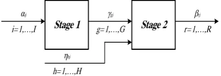
Network DMUs have various types of structure such as basic two-stage, general two-stage, se-ries, parallel, mixed, hierarchical, and dynamic. It should be noted that among the structures that have been mentioned, the two-stage struc-ture has been widely discussed in the NDEA lit-erature [13]. Accordingly, in this study, window network DEA model will proposed based on ex-tended two-stage structure presented in Fig. 1. As can be seen in Fig. 1, the network structure

Stage 1 Stage 2

αij

i=1, ,I

γgj

g=1, ,G

βrj

r=1, ,R

ηhj

h=1, ,H

(3)

is a two-stage process with added inputs to the second stage, where there is a set of ri

homoge-nous DMUj(j = 1,· · ·, n) that each DMU has I

inputsαij(i= 1,· · ·, I) in the first stage, G

inter-mediate variables γgj(g = 1,· · ·, G) that linking

first stage and second stage, H additional inputs

ηhj(h= 1,· · ·, H) in the second stage and finally R outputsβrj(r = 1,· · ·, R) in the second stage.

Note that the NDEA models, like the classic DEA models could be proposed based on differ-ent return to scale (RTS) including constant re-turn to scale (CRS) and variable rere-turn to scale (VRS) assumptions that presented by Charnes et al. [6] and Banker et al. [3], respectively. Since, the VRS is a realistic assumption in different ap-plication and real word problems, the modeling of NDEA in this section and subsequently modeling of WNDEA in next section are presented under VRS assumption.

Table 1: The Value of Parameters in WNDEA Model

Parameters Value Number of DMUs 5 Number of Periods 5 Width of Window 2 Number of Windows 4

Stage 1

Operational Management Process

Stage 2

Portfolio Management

Process Financial Fees

General & Administrative Fees

Asset Turnover

Standard Deviation

Net Asset Value Average Return

Figure 2: Extended Two-Stage Process

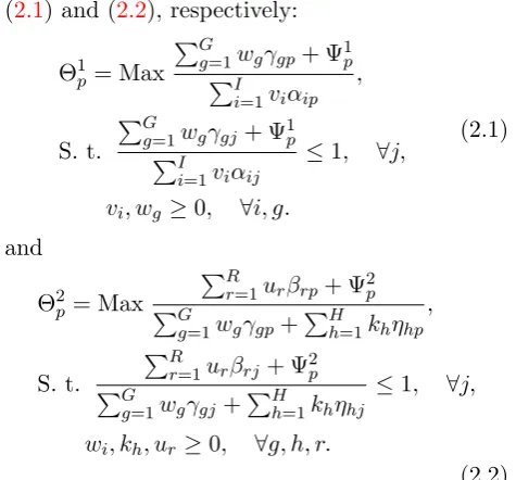
Now, after providing the necessary preliminar-ies, modeling the network data envelopment anal-ysis based on additive efficiency decomposition approach that presented by Chen et al. [8], will be discussed. Acording to the BCC model that intruduced by Banker et al. [3], the efficiency scores based on varibele return to sclae assum-tion for DMU under investigaassum-tion in the stages 1 and 2 can be estimated by the following Models

(2.1) and (2.2), respectively:

Θ1_p = Max

∑G

g=1wgγgp+ Ψ1p

∑I

i=1viαip ,

S. t.

∑G

g=1wgγgj+ Ψ1p

∑I i=1viαij

≤1, ∀j,

vi, wg ≥0, ∀i, g.

(2.1)

and

Θ2_p= Max

∑R

r=1urβrp+ Ψ2p

∑G

g=1wgγgp+

∑H

h=1khηhp ,

S. t.

∑R

r=1urβrj+ Ψ2p

∑G

g=1wgγgj+ ∑H

h=1khηhj

≤1, ∀j,

wi, kh, ur≥0, ∀g, h, r.

(2.2) Based upon the idea of Chen et al. [8], the overall efficiency of the two-stage process with added inputs to the second stage will be defined as Eq. (2.3):

Θp =λ1Θ1p+λ2Θ2p

=λ1

(∑G

g=1wgγgp+ Ψ1p

∑I

i=1viαip )

+λ2

( _∑_R

r=1urβrp+ Ψ2p

∑G

g=1wgγgp+

∑H

h=1khηhp

)

(2.3)

Note that in Eq. (2.3), λ1 and λ2 are

user-specified weights such thatλ1+λ2 = 1 . In other

words, λ1 and λ2 are the relative importance of

the performances of first stage and second stage, respectively, to the overall performance of the decision-making unit. Accordingly, the overall ef-ficiency of the process is calculated by solving the Model (2.4) as follows:

Θp=Maxλ1

(∑G

g=1wgγgp+ Ψ1p

∑I

i=1viαip

)

+λ2

( _∑_R

r=1urβrp+ Ψ2p

∑G

g=1wgγgp+

∑H

h=1khηhp

)

,

S.t.

∑G

g=1wgγgj+ Ψ1p

∑I i=1viαij

≤1, ∀j,

∑R

r=1urβrj + Ψ2p

∑G

g=1wgγgj+ ∑H

h=1khηhj ∀j,

vi, wg, kh, ur≥0, ∀i, g, h, r.

(4)

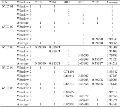
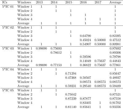
Table 2: The Results of Window Network DEA Model - Overall

ICs Windows 2013 2014 2015 2016 2017 Average

5*IC 01 Window 1 1 1 1

Window 2 1 1 1

Window 3 1 1 1

Window 4 1 1 1

Average 1 1 1 1 1 1

5*IC 02 Window 1 1 1 1

Window 2 1 1 1

Window 3 1 1 1

Window 4 1 0.99290 0.99645

Average 1 1 1 1 0.99290 0.99858 5*IC 03 Window 1 0.99690 0.83923 0.91807

Window 2 0.82803 1 0.91402

Window 3 1 0.59596 0.79798

Window 4 0.68208 0.75637 0.71923 Average 0.99690 0.83363 1 0.63902 0.75637 0.84518

5*IC 04 Window 1 1 1 1

Window 2 1 0.71294 0.85647

Window 3 0.64944 0.50507 0.57725 Window 4 0.59205 0.59205 0.59205 Average 1 1 0.68119 0.54856 0.59205 0.76436

5*IC 05 Window 1 1 1 1

Window 2 1 0.84627 0.92314

Window 3 0.87239 0.87877 0.87558

Window 4 0.83742 1 0.91871

Average 1 1 0.85933 0.85809 1 0.94348

As it can be seen in Model (2.4), this model cannot be turned into a linear program (LP) by applying the usual Charnes and Cooper [4]. For eliminating this issue, Chen et al. [8] suggested and as Eq. (2.5) Eq. (2.6), respectively:

λ1=

∑I i=1viαip ∑I

i=1viαip+∑Gg=1wgγgp+ ∑H

h=1khηhp

(2.5)

λ1=

∑G

g=1wgγgp+ ∑H

h=1khηhp ∑I

i=1viαip+∑Gg=1wgγgp+ ∑H

h=1khηhp

(2.6)

Thus, by utilizing the above equations, Model (2.4) will be converted to Model (2.7) as follows:

Θp=Max

∑G

g=1wgγgp+ Ψ1p+

∑R

r=1urβrp+ Ψ2p

∑R

i=1viαip+

∑G

g=1wgγgp+

∑H

h=1khηhp

S.t.

∑G

g=1wgγgj+ Ψ1p

∑I i=1viαij

≤1, ∀j,

(2.7)

∑R

r=1urβrj+ Ψ2p

∑G

g=1wgγgj+

∑H

h=1khηhj ∀j,

vi, wg, kh, ur≥0, ∀i, g, h, r.

Now, by applying Charnes and Cooper [4] transformation, Model (2.7) is equivalent to Model (2.8):

Θp=Max G

∑

g=1

wgγgp+ Ψ1p+ R

∑

r=1

urβrp+ Ψ2p,

S.t.

R

∑

i=1

viαip+ G

∑

g=1

wgγgp+ H

∑

h=1

khηhp= 1,

G

∑

g=1

wgγgj− R

∑

i=1

viαij + Ψ1p ≤0 ∀j,

R

∑

r=1

urβrj− G

∑

g=1

wgγgj

(5)

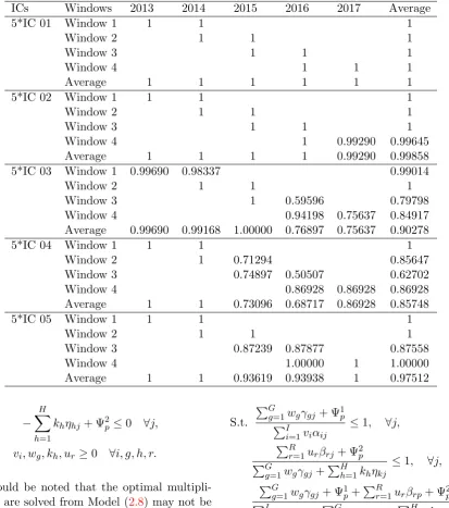
Table 3: The Results of Window Network DEA Model - Stage 1

5*IC 01 Window 1 1 1 1

Window 2 1 1 1

Window 3 1 1 1

Window 4 1 1 1

Average 1 1 1 1 1 1

5*IC 02 Window 1 1 1 1

Window 2 1 1 1

Window 3 1 1 1

Window 4 1 0.99290 0.99645

Average 1 1 1 1 0.99290 0.99858 5*IC 03 Window 1 0.99690 0.98337 0.99014

Window 2 1 1 1

Window 3 1 0.59596 0.79798

Window 4 0.94198 0.75637 0.84917 Average 0.99690 0.99168 1.00000 0.76897 0.75637 0.90278

5*IC 04 Window 1 1 1 1

Window 2 1 0.71294 0.85647

5*IC 05 Window 1 1 1 1

Window 2 1 1 1

Window 3 0.87239 0.87877 0.87558

Window 4 1.00000 1 1.00000

Average 1 1 0.93619 0.93938 1 0.97512

− H

∑

h=1

khηhj + Ψ2p≤0 ∀j,

vi, wg, kh, ur≥0 ∀i, g, h, r.

It should be noted that the optimal multipli-ers that are solved from Model (2.8) may not be unique. As a result, the decomposition of the overall efficiency defined in Eq. (2.3) would not be unique. Kao and Hwang [14] suggested an ap-proach to find a set of multipliers which produces the maximum efficiency score for stage 1 (or stage 2) while maintaining the overall efficiency score. By assuming that the efficiency of the stage 1 is more important for the decision maker (DM), Θ1_p will be estimated by solving Model (2.9) while calculating the Θp by Model (2.8).

Θ1_p =Max

∑G

g=1wgγgp+ Ψ1p

∑I

i=1viαip

(2.9) S.t.

∑G

g=1wgγgj+ Ψ1p

∑I i=1viαij

≤1, ∀j,

∑R

r=1urβrj + Ψ2p

∑G

g=1wgγgj+

∑H

h=1khηkj

≤1, ∀j,

∑G

g=1wgγgj+ Ψ1p+

∑R

r=1urβrp+ Ψ2p

∑I

i=1viαip+

∑G

g=1wgγgp+ ∑H

h=1khηkp

= Θ∗_p,

vi, wg, kh, ur≥0 ∀i, g, h, r.

Since Model (2.9) is a linear fractional pro-gram, using the transformation of Charnes and Cooper [4], this model will be equivalent to Model (2.10):

Θ1_p =Max

G

∑

g=1

wgγgp+ Ψ1p,

S.t.

I

∑

i=1

viαip= 1,

(6)

Table 4: The Results of Window Network DEA Model - Stage 2

5*IC 01 Window 1 1 1 1

Window 2 1 1 1

Window 3 1 1 1

Window 4 1 1 1

Average 1 1 1 1 1 1

5*IC 02 Window 1 1 1 1

Window 2 1 1 1

Window 3 1 0.64790 0.82395

Window 4 0.45024 0.50000 0.47512 Average 1 1 1 0.54907 0.50000 0.80981 5*IC 03 Window 1 0.99690 0.75693 0.87692

Window 2 0.78612 1 0.89306

Window 3 1 0.59596 0.79798

Window 4 0.14049 0.75637 0.44843 Average 0.99690 0.77153 1 0.36822 0.75637 0.77861

5*IC 04 Window 1 1 1 1

Window 2 1 0.71294 0.85647

5*IC 05 Window 1 1 1 1

Window 2 1 0.75042 0.87521

Window 3 0.87239 0.87877 0.87558

Window 4 0.83405 1 0.91702

Average 1 1 0.81140 0.85641 1 0.93356

Table 5: The Average Efficiency Score and Ranking of Investment Companies

2*ICs Overall Stage 1 Stage 2

Average Efficiency Rank Average Efficiency Rank Average Efficiency Rank

IC 01 1 1 1 1 1 1

IC 02 0.99858 2 0.99858 2 0.80981 3 IC 03 0.84518 4 0.90278 4 0.77861 4 IC 04 0.76436 5 0.85748 5 0.59489 5 IC 05 0.94348 3 0.97512 3 0.93356 2

G

∑

g=1

wgγgj− I

∑

i=1

viαij + Ψ1p ≤0 ∀j,

R

∑

r=1

urβrj − G

∑

g=1

wgγgj

− H

∑

h=1

khηhj+ Ψ2p ≤0, ∀j,

G

∑

g=1

wgγgp+ R

∑

r=1

urβrp−Θ∗p

(_∑G

g=1

wgγgp

+

H

∑

h=1

khηhp

)

+ Ψ1_p+ Ψ2_p= Θ∗_p,

vi, wg, kh, ur≥0 ∀i, g, h, r.

After calculating Θ1_p∗ using the Model (2.10), the efficiency score of the stage 2 is obtained from Eq. (2.11):

Θ2_p∗= θ

∗

p−λ∗1Θ1p∗

λ∗₂ (2.11)

(7)

more important for the DM, Θ2_pwill be estimated by solving the Model (2.12) while calculating the Θ∗_p by Model (2.8).

Θ2p=Max

∑R

r=1urβrp+ Ψ2p ∑G

g=1wgγgp+∑Hh=1khηhp

S.t.

∑G

g=1wgγgj+ Ψ1p ∑I

i=1viαij

≤1, ∀j,

∑R

r=1urβrj+ Ψ 2 p ∑G

g=1wgγgj+ ∑H

h=1khηkj

≤1, ∀j,

∑G

g=1wgγgp+ Ψ1p+ ∑R

r=1urβrp+ Ψ2p ∑I

i=1viαip+ ∑G

g=1wgγgp+ ∑H

h=1khηkp

= Θ∗p,

vi, wg, kh, ur≥0 ∀i, g, h, r.

(2.12)

Like the previous fractional models in this sec-tion, by employing the Charnes and Cooper [4] transformation, Model (2.12) will be equivalent to Model (2.13):

Θ2_p =Max

R

∑

r=1

urβrp+ Ψ2p,

S.t.

G

∑

g=1

wgγgp+ H

∑

h=1

khηhp= 1,

G

∑

g=1

wgγgj− I

∑

i=1

viαij+ Ψ1p ≤0 ∀j,

R

∑

r=1

urβrj− G

∑

g=1

wgγgj

− H

∑

h=1

khηhj + Ψ2p≤0, ∀j,

G

∑

g=1

wgγgp+ R

∑

r=1

urβrp−Θ∗p

( _I

∑

i=1

viαip

)

+ Ψ1_p+ Ψ2_p= Θ∗_p,

vi, wg, kh, ur ≥0 ∀i, g, h, r.

(2.13) Finally, after Θ2_p∗ is calculated from the Model (2.13), the efficiency score of the stage 1 is ob-tained from Eq. (2.14):

Θ1_p∗= θ

∗

p−λ∗2Θ2p∗

λ∗₁ (2.14)

It should be noted that the two-stage data en-velopment analysis models presented in this sec-tion are input-oriented. The window network

data envelopment analysis model for a two-stage process with added inputs to the second stage un-der VRS assumption will be proposed in the next section.

3 Window Network Data

Envel-opment Analysis

The combination of window analysis approach and DEA models is a very applicable and useful methodology to investigate the dynamic changes of the efficiency of each DMU comprehensively, both horizontally and vertically. The goal of this section is to propose window network DEA model for dynamic performance measurement of net-work DMUs that is capable to be used in the presence of panel data for performance appraisal of DMUs with network structure. In order to propose WNDEA model, consider an extended two-stage process with added inputs to the sec-ond stage as depicted in Fig. 1, as well as the indices, parameters and variables that introduced in previous section. Note that, in window analysis methodology, the same DMU in different period of time are considered as entirely different DMUs and moving average approach is used to choose different reference sets in order to measure the relative efficiency of each DMU.

Accordingly, consider a set of ri DMUs with

two-stage structure in T(t = 1,· · ·, T) period of time. Let indices of qz denote the window start at the time point of q and the width of window is z(1 ≤ z ≤ T −q), Λqz is the set of DMUs

that exists in window with characteristics of qz. The window two-stage DEA model for measuring the overall efficiency of the process is proposed as Model (3.15):

Θpqz=Max G ∑

g=1

wgγgpqz+ Ψ1pqz+ R ∑

r=1

urβrpqz+ Ψ2pqz,

S.t.

R ∑

i=1

viαipqz+ G ∑

g=1

wgγgpqz+ H ∑

h=1

khηhpqz= 1,

G ∑

g=1

wgγgjt− I ∑

i=1

viαijt+ Ψ1pqz≤0 ∀j, t∈Λqz

R ∑

r=1

urβrjt− G ∑

g=1 wgγgjt

(8)

− H ∑

h=1

khηhjt+ Ψ2p≤0 ∀j, t∈Λqz

vi, wg, kh, ur≥0 ∀i, g, h, r.

As the previous section, if first sub process is as-sumed to be more important, Θ1(pqz) will be

cal-culated by solving the Model (3.16) while measur-ing the Θ∗(pqz) by Model (3.15).

Θ1_pqz =Max

G

∑

g=1

wgγgpqz+ Ψ1pqz,

S.t.

I

∑

i=1

viαipqz= 1,

G

∑

g=1

wgγgjt− I

∑

i=1

viαijt

(3.16)

+ Ψ1_pqz ≤0 ∀j, t∈Λqz, R

∑

r=1

urβrjt− G

∑

g=1

wgγgjt

− H

∑

h=1

khηhjt+ Ψ2pqz ≤0,∀j, t∈Λqz,

G

∑

g=1

wgγgpqz+ R

∑

r=1

urβrpqz

−Θ∗_pqz

 ∑G

g=1

wgγgpqz+ H

∑

h=1

khηhpqz

 

+ Ψ1_pqz+ Ψ2_pqz = Θ∗_pqz, vi, wg, kh, ur ≥0 ∀i, g, h, r.

And the efficiency of the second sub process is calculated by Eq. (3.17):

Θ2_pqz∗ = θ

∗

pqz−λ∗1Θ1pqz∗

λ∗₂ (3.17)

In a similar manner, if second sub process is as-sumed to be more important, Θ2_pqz will be esti-mated by solving the Model (3.18) while

measur-ing the Θ∗_pqz by Model (3.15).

Θ2_pqz =Max

R

∑

r=1

urβrpqz+ Ψ2pqz,

S.t.

G

∑

g=1

wgγgpqz+ H

∑

h=1

khηhpqz = 1,

G

∑

g=1

wgγgjt− I

∑

i=1

viαijt

+ Ψ1_pqz ≤0 ∀j, t∈Λqz, R

∑

r=1

urβrjt− G

∑

g=1

wgγgjt− H

∑

h=1

khηhjt

+ Ψ2_pqz ≤0, ∀j, t∈Λqz, G

∑

g=1

wgγgpqz+ R

∑

r=1

urβrpqz

−Θ∗_pqz

( _I ∑

i=1

viαipqz

)

+ Ψ1_pqz + Ψ2_pqz = Θ∗_pqz, vi, wg, kh, ur≥0 ∀i, g, h, r.

(3.18)

And the efficiency of the first sub process is then calculated as follows:

Θ1_pqz∗ = θ

∗

pqz−λ∗2Θ2pqz∗

λ∗₁ (3.19)

It should be noted that applying the WNDEA model required to choose the window and the number of windows depends on the time span considered. A real-life case study from financial market is applied to demonstrate the applicabil-ity, efficacy and effectiveness of the proposed WN-DEA model.

4 Application:

Investment

Company

(9)

in the investment incomes and risks in proportion to his/her interest in the ICs [16]. As a result, the activities of investment companies can be viewed as a two-stage process that the management of ICs seeks to attract funds from investors in stage 1, and focuses on the optimal portfolio construc-tion in stage 2. Fig.2depicts the empirical frame-work of the activities of ICs.

As shown in Fig. 2, the overall efficiency of the ICs is decomposed into two stages that the first stage indicates the operational management pro-cess and the second stage indicates the portfolio management process. In the first stage, two in-put variables including financial fees and general and administrative fees are considered. Net as-set value (NAV) is the intermediate measure that is linking first and second stage. In the second stage, asset turnover and standard deviation of the returns are the input variables and average return is the output variable.

Now, for employing the WNDEA model in or-der to performance assessment of 5 ICs from Tehran stock exchange during the period 2013– 2017, a 2 year window width was chosen and therefore four overlapping windows will be an-alyzed over the 5 year study period. The value of parameters that used in WNDEA model are given in Table 1.

Now, by assuming that the first stage is more important for DM, the results of window network DEA model for overall, stage 1 and stage 2, will be calculated using Model (3.15), Model (3.16) and Equation (3.17), respectively. It should be noted that LINGO software was used for solving all models. Accordingly, Tables 2 to 4, present the overall, first stage and second stage efficiency based on WNDEA approach, respectively.

As can be seen in Tables 2 to 4, in addition to calculating the efficiency of each IC per win-dow, three types of average efficiency including the average efficiency scores of ICs for all years, the average efficiency scores of ICs for all windows and the average of all efficiency scores for each IC are measured. Accordingly, in order to evaluate and rank all ICs comprehensively, the average of all efficiency scores for each IC are extracted from Tables 2to4 and summarized in Table5.

Numerical assessment of the proposed window network DEA model during period from 2013 to

2017 reveals that the presented model is able to highlight the investment companies that may have managed their portfolios well. Also, which of the two-stage including operational manage-ment process and portfolio managemanage-ment process, may have been the contributory factor to their good or bad performance.

With respect to the results from WNDEA model, the IC 01 is the best investment company in comparison to other ICs in period 2013–2017. It should be noted that the introduced informa-tion of Table 5 can help investors to make in-formed decisions and enables administrators of investment companies to judge how well their portfolio managers have performed relative to their competitors over the period 2013–2017.

5 Conclusion

This study presents a window network data en-velopment analysis model based on additive effi-ciency decomposition and VRS assumptions for assessing the relative performance of investment companies. It should be noted that this WNDEA model is presented for extended two-stage struc-ture with added inputs to the second stage. The applicability of the WNDEA model is demon-strated by performance measurement of 5 invest-ment companies from Tehran Stock Exchange across the period 2013–2017. For future research, the WNDEA method can be extended based on uncertainty programming approaches for dealing with uncertain panel data (for more details see [17,18,19]). Moreover, the window network DEA model can also be applied to other financial in-stitutions with network structure, such as banks and insurance companies.

References

[1] A. Al-Refaie, R. Najdawi, E. Sy, Using DEA window analysis to measure the efficiencies of blowing machines in plastics industry, Jor-dan Journal of Mechanical and Industrial Engineering 10 (2016) 1-11.

(10)

envelopment analysis-DEA (window model),

Indian Journal of Fundamental and Applied Life Sciences 5 (2015) 1291-1297.

[3] R. D. Banker, A. Charnes, W. W. Cooper, Some models for estimating technical and scale inefficiencies in data envelopment anal-ysis, Management Science 30 (1984) 1078-1092.

[4] A. Charnes, W. W. Cooper, Programming with linear fractional functionals,Naval Re-search Logistics Quarterly 9 (1962) 181-186. [5] A. Charnes, W. W. Cooper, B. Golany, A development study of DEA in measuring the effect of maintenance units in the US Air Force, Annals of Operations Research 2 (1985) 95-112.

[6] A. Charnes, W. W. Cooper, E. Rhodes, Measuring the efficiency of decision making units, European Journal of Operational Re-search 2 (1978) 429-444.

[7] X. Chen, Y. Gao, Q. An, Z. Wang, L. Nerali, ). Energy efficiency measurement of Chinese Yangtze River Deltas cities transportation: a DEA window analysis approach,Energy Ef-ficiency (2018) 1-13.

[8] Y. Chen, W. D. Cook, N. Li, J. Zhu, Ad-ditive efficiency decomposition in two-stage DEA, European Journal of Operational Re-search 196 (2009) 1170-1176.

[9] A. Flokou, V. Aletras, D. Niakas, A window-DEA based efficiency evaluation of the pub-lic hospital sector in Greece during the 5-year economic crisis,PloS One12 (2017) 177-194. [10] G. E. Halkos, M. L. Polemis, The impact of economic growth on environmental efficiency of the electricity sector: A hybrid window DEA methodology for the USA, Journal of Environmental Management211 (2018) 334-346.

[11] A. Hemmasi, M. Talaeipour, H. Khademi-Eslam, S. H. Pourmousa, Using DEA win-dow analysis for performance evaluation of Iranian wood panels industry, African Jour-nal of Agricultural Research 6 (2011) 1802-1806.

[12] T. Jia, H. Yuan, The application of DEA (Data Envelopment Analysis) window anal-ysis in the assessment of influence on opera-tional efficiencies after the establishment of branched hospitals, BMC Health Services Research 17 (2017) 265-275.

[13] C. Kao, Network data envelopment analysis: A review, European Journal of Operational Research 239 (2014) 1-16.

[14] C. Kao, S. N. Hwang, Efficiency decomposi-tion in two-stage data envelopment analysis: An application to non-life insurance compa-nies in Taiwan, European Journal of Oper-ational Research 185 (2008) 418-429.

[15] Y. Ohe, N. Peypoch, Efficiency analysis of Japanese Ryokans: A window DEA ap-proach, Tourism Economics 22 (2016) 1261-1273.

[16] P. Peykani, E. Mohammadi, Interval net-work data envelopment analysis model for classification of investment companies in the presence of uncertain data, Journal of In-dustrial and Systems Engineering 11 (2018) 63-72.

[17] P. Peykani, E. Mohammadi, A. Jab-barzadeh, A. Jandaghian, Utilizing robust data envelopment analysis model for measur-ing efficiency of stock, a case study: Tehran stock exchange, Journal of New Research in Mathematics 1 (2016) 15-24.

[18] P. Peykani, E. Mohammadi, M. S. Pishvaee, M. Rostamy-Malkhalifeh, A. Jabbarzadeh, A novel fuzzy data envelopment analysis based on robust possibilistic programming: possibility, necessity and credibility-based approaches,RAIRO-Operations Research 52 (2018) 1445-1463.

(11)

[20] D. Pjevevi, A. Radonji, Z. Hrle, V. oli, DEA window analysis for measuring port efficien-cies in Serbia, Promet-Traffic & Transporta-tion 24 (2012) 63-72.

[21] M. Pulina, C. Detotto, A. Paba, An investi-gation into the relationship between size and efficiency of the Italian hospitality sector: A window DEA approach,European Journal of Operational Research 204 (2010) 613-620. [22] A. Salem Al-Eraqi, A. Mustafa, A. Tajudin

Khader, An extended DEA windows analy-sis: Middle East and East African seaports,

Journal of Economic Studies 37 (2010) 208-218.

[23] K. Wang, S. Yu, W. Zhang, Chinas regional energy and environmental efficiency: A DEA window analysis based dynamic evaluation,

Mathematical and Computer Modelling 58 (2013) 1117-1127.

[24] R. Webb, Levels of efficiency in UK retail banks: a DEA window analysis, Interna-tional Journal of the Economics of Business

10 (2003) 305-322.

[25] Q. D. Wu, Y. Shi, Q. Xia, W. D. Zhu, Effec-tiveness of the policy of circular economy in China: A DEA-based analysis for the period of 11th five-year-plan, Resources, Conser-vation and Recycling 83 (2014) 163-175. [26] H. H. Yang, C. Y. Chang, Using DEA

win-dow analysis to measure efficiencies of Tai-wan’s integrated telecommunication firms,

Telecommunications Policy 33 (2009) 98-108.

Pejman Peykani is a PhD Candi-date at the School of Industrial En-gineering, Iran University of Sci-ence and Technology, Tehran, Iran. He received his MSc in Financial Engineering in 2014 from the K. N. Toosi University of Technology, Tehran, Iran. His areas of research interests include Data Envelopment Analysis, Financial

Modeling, Portfolio Management, Robust Opti-mization, and Fuzzy Mathematical Programing.