STREAMLINE UPWIND/PETROV GALERKIN SOLUTION OF OPTIMAL CONTROL PROBLEMS GOVERNED BY TIME DEPENDENT DIFFUSION-CONVECTION-REACTION EQUATIONS

STREAMLINE UPWIND/PETROV GALERKIN SOLUTION OF OPTIMAL CONTROL PROBLEMS GOVERNED BY TIME DEPENDENT DIFFUSION-CONVECTION-REACTION EQUATIONS

T. AKMAN1_{, B. KARAS ¨OZEN}2_{, Z. KANAR-SEYMEN}2_{, §}

Abstract. The streamline upwind/Petrov Galerkin (SUPG) finite element method is studied for distributed optimal control problems governed by unsteady diffusion-convection-reaction equations with control constraints. We derive stability and convergence esti-mates for fully-discrete state, adjoint and control and discuss the choice of the stabiliza-tion parameter by applying backward Euler method in time. We show that by balancing the error terms in the convection dominated regime, optimal convergence rates can be obtained. The numerical results confirm the theoretically observed convergence rates. Keywords: optimal control problems, unsteady diffusion-convection-reaction equations, finite element elements, a priori error estimates.

AMS Subject Classification: 49N10,49K20, 65M60,65M15.

1. Introduction

Optimal control problems (OCPs) governed by diffusion-convection-reaction equations arise in environmental control problems, like air and water pollution, optimal control of fluid flow, steel formation and in many other industrial applications. It is well known that the standard Galerkin finite element discretization causes nonphysical oscillations in the solution when convection dominates. Stable and accurate numerical solutions can be achieved by various effective stabilization techniques such as the streamline upwind/Petrov Galerkin (SUPG) finite element method [6], the local projection stabilization [3], the edge stabilization [11] and the symmetric stabilization [4].

In the recent years, most of the research is concentrated on parabolic OCPs. There are few publications dealing with the OCPs governed by non-stationary diffusion-convection-reaction equations. For example, the local discontinuous Galerkin (dG) approximation and the characteristic finite element solution of the control constraint OCP are discussed in [10, 17], respectively. The symmetric interior penalty Galerkin method with backward Euler time discretization is studied in [1]. SUPG discretization of a time-dependent diffusion-convection-reaction equation and a priori error analysis are given in [12].

1

Department of International Trade And Finance, Faculty of Management, University of Turkish Aeronautical Association, 06790, Etimesgut, Ankara, Turkey.

e-mail: [email protected], ORCID1: http://orcid.org/0000-0003-1206-2287;

2 _{Department of Mathematics & Institute of Applied Mathematics, Middle East Technical University,}

Ankara, Turkey.

e-mail: [email protected], [email protected];

ORCID2,2: http://orcid.org/0000-0003-1037-5431, http://orcid.org/0000-0001-8391-8121;

§ Manuscript received: August 03, 2016; accepted: September 20, 2016.

TWMS Journal of Applied and Engineering Mathematics, Vol.7, No.2; cI¸sık University, Department of Mathematics, 2017; all rights reserved.

The choice of the stabilization parameter for time-dependent diffusion-convection-reaction equation is discussed in [12] for SUPG discretization in space, backward Euler and Crank-Nicolson method in time. When the stabilization parameter is chosen proportional to the mesh size h, i.e. τ = O(h), for all cells, the discrete solution converges for the time-continuous case. When discretization is performed first in time, then the stabilization parameter can be chosen proportional to the time step k. However, this leads to large spurious oscillations. When the time and space grids are comparable, i.e. k ∼ h, then the stabilization parameter can be chosen as for the steady-state case, whereas the spatial and temporal errors have to be balanced.

Our work is motivated by the study [12] where the SUPG-backward Euler discretization is studied for a single parabolic partial differential equation (PDE). We have discretized the OCP using SUPG in space and backward Euler method in time by extending the error analysis for evolutionary convection-diffusion-reaction equations provided in [12] to OCPs governed by time-dependent convection-diffusion-reaction equations. According to [9, 10], the characteristic finite element method combined with backward Euler discretization leads to the first order of convergence with the choice ofh=k. Here, we choose the stabilization parameter depending on the length of the time step to balance the error terms for the convection-dominated regime. It turns out that the SUPG improves the convergence rates up to the orderO(h4/3_{) withk}∼_=h4/3 _{and the oscillations in the solutions disappear. The} theoretically observed convergence rates are confirmed by the numerical results.

The rest of the paper is organized as follows. In Section 2, we define the model problem and derive the optimality system. In Section 3, we present the SUPG finite element method and state the semi-discrete optimality system. In Section 4, stability and convergence estimates for the fully discrete optimality system are presented and the choice of the stabilization parameter is discussed. In Section 5, numerical results are presented for different choices of stabilization parameters. The paper ends with some conclusions.

2. The Optimal Control Problem

We adopt the standard notations for Sobolev spaces on computational domains and their norms. Ω and ΩU are bounded convex polygonal domains inR2 with Lipschitz boundaries

∂Ω and ∂ΩU, respectively. We consider the following distributed optimal control problem

governed by the unsteady diffusion-convection-reaction equation with control constraints

minimize

u∈Uad_⊆L2_(0,T;L2_(ΩU))J(y, u) :=

1 2

Z T

0

ky−ydk2L2_(Ω) +αkuk2_L2_(ΩU)

dt, (1a)

subject to ∂ty−∆y+β· ∇y+σy=f+Bu, (x, t)∈Ω×(0, T], (1b)

y(x, t) = 0, (x, t)∈∂Ω×(0, T], (1c) y(x,0) =y0(x), x∈Ω, (1d)

Uad=u∈L2(0, T;L2(ΩU) : ua≤u≤ub a.e. in ΩU ×(0, T] , (2)

For well-posedness of the optimal control problem (1) we refer to [1, 9, 10].

The variational formulation corresponding to (1) is given by

minimize

u∈Uad J(y, u) := 1 2

Z T

0

ky−ydk2L2_(Ω)+αkuk2_L2_(ΩU)

dt, (3a)

subject to (∂ty, v) +a(y, v) +b(u, v) = (f, v) ∀v∈V, t∈(0, T], (3b)

y(x,0) =y0,

a(y, v) =

Z

Ω

(∇y∇v+β· ∇yv+σyv)dx, b(u, v) =−

Z

Ω

Buvdx, (f, v) =

Z

Ω f vdx.

It is well known that the triple (y, u, p) is the unique solution of (3) if and only if there is an adjointp(x, t) such that (y, p, u) satisfies the following optimality system [1, 2]:

(∂ty, v) +a(y, v) +b(u, v) = (f, v), ∀v∈V, y(x,0) =y0, (4a)

−(∂tp, ψ) +a(ψ, p) =−(y−yd, ψ), ∀ψ∈V, p(x, T) = 0, (4b)

Z T

0

(αu−B∗p, w−u)U dt≥0, ∀w∈Uad, (4c)

whereB∗ denotes the adjoint ofB.

3. Streamline Upwind/Petrov Galerkin(SUPG) Finite Element Method for Optimal Control Problem

Let{T_h}be a triangulation of Ω such that Ω =∪_K∈ThK,Ki∩Kj =∅forKi, Kj ∈Th, i 6= j. The diameter of an element K and the length of an edge E are denoted by hK

and hE, respectively. In addition, the maximum value of element diameter is denoted by

h = max

K∈Th

hK. We note that the subindexU denotes the associated triangularization for

the control. In general, the sizes of the elements in {(T_h)U}h are smaller than those in

{Th}h, so we assume thathU/h≤C throughout this paper [9, Sec.3].

We use piecewise continuous linear finite element space to define the discrete spaces of the state, the adjoint and the control

Vh=

v∈H₀1(Ω) : v|_K∈_P1_{(K) ∀K∈T}

h ,

Uh =

u∈L2(ΩU) : u|KU∈P 1_(K

U) ∀KU ∈(Th)U .

Finite element approximations of the state, the adjoint and the control are given as

yh(x, t) = m−1

X

i=1

yh,i(t)ϕi(x), ph(x, t) = m−1

X

i=1

ph,i(t)ϕi(x), uh(x, t) = mu

X

i=0

uh,i(t)φi(x),

yh(t) = (yh,1(t), . . . , yh,m−1(t))T, ph(t) = (ph,1(t), . . . , ph,m−1(t))T, uh(t) = (uh,0(t), . . . , uh,mu(t))

T_.

The semi-discrete approximation of the optimal control problem (3) is defined as follows:

minimize

uh∈Uhad

Z T

0 1 2

X

K∈Th

ky_h−yd,hk2L2_(K)+

α 2

X

KU∈TUh

ku_hk2_L2_(KU)

dt, (5a)

subject to (∂tyh, vh) + X

K∈Th

τ(∂tyh, β· ∇vh)K+ash(yh, vh) +bsh(uh, vh) = (f, vh)sh, (5b)

as_h(y, vh) =a(y, vh) + X

K∈Th

τ(−∆y+β· ∇y+σy, β· ∇v_h)K, (6a)

bs_h(u, vh) =b(u, vh)− X

K∈Th

τ(Bu, β· ∇v_h)K, (6b)

(f, vh)sh= (f, vh) + X

K∈Th

τ(f, β· ∇v_h)K. (6c)

The stabilization parameter τ is chosen depending on a priori error estimates in Sec-tion 4. We use discretize-then-optimize approach to solve the OCP. We derive the fully-discrete optimality system by differentiating the fully-discrete Lagrangian with respect to the state, adjoint and control variables. The semi-discrete optimality system is discretized in time with the backward Euler method and resulting fully discrete optimality system is solved using all all at once approach [15] with the MINRES. The fully discrete optimality system is given as:

minimize

un h∈Uhad





k 2

X

K∈Th

ky_hn−y_d,hn k2_L2_(K)+α

k 2

X

KU∈Tuh

kun_hk2_L2_(KU) 

 (7)

(yn_h−yn_h−1, ϕ) +kas_h(y_hn, ϕ) =k(fn+Bun_h, ϕ) +k



 X

K∈Th

τ(fn+Bun_h, β· ∇ϕ)_K





−



 X

K∈Th

τ(yn_h−yn_h−1, β· ∇ϕ)K 

, ∀ϕ∈V_h, n= 1, . . . , N+ 1, (8a)

(ψ, pn_h−1−pn_h) +kas_h ψ, pn_h−1 =−k(y_hn−1−y_d,hn−1), ψ−k



 X

K∈Th

τ(ψ, β· ∇(pn_h−1−pn_h))K 

,∀ψ∈Vh, n=N + 1, . . . ,2,

(8b)

(αun_h−B∗p_hn−1−τ β· ∇B∗pn_h−1, wh−unh)U ≥0, ∀wh ∈Uhad, n= 1, . . . , N+ 1. (8c)

4. A Priori Error Estimates

In this section, we shall derive the stability and convergence estimates for the fully-discrete OCP. We start with the stability estimates following the approach in [12] for time-dependent diffusion-convection-reaction equations. In this section, r denotes the degree of local polynomials andk · kr denotes the norm in Hr(Ω) with H0(Ω) = L2(Ω).

To prove the a priori error estimate of the fully-discrete scheme, we need the discrete time-dependent norm for 1≤q <∞ by [9],

kvk_Lq_(0,T;L2_(Ω)) =

N+1

X

n=1

kkvnkq_L2_(Ω) !1/q

4.1. Stability Estimates. We take a fixed time step k, and we denote the fully discrete state, adjoint and control solution at timetn=nk by yhn, pnh and unh, respectively.

More-over, the exact solutions of the state, the adjoint and the control at timetn are defined as

yn,pn and un, respectively. We give first some useful inequalities which are needed. The elliptic projection πh:V →Vh is defined by (∇(y−πhy),∇vh) = 0 for all vh∈Vh

and

(πhy)t=πh(yt) =πhyt. (9)

The following inverse inequality holds for each vh ∈Vh with the assumption of a quasi

uniform mesh (see, e.g., [5]):

kv_hk_Wm,q_(K)≤c_invh

l−m−d(1 q0−

1

q)

K kvhkWl,q0_(K), (10)

where 0 ≤ l ≤ m ≤ 1, 1 ≤ q0 ≤q ≤ ∞, h_K is the mesh size diameter of K ∈ T_h. We note that we take the same step sizehK =h for all mesh cellK. The interpolation error

estimate fory∈V ∩Hr+1 given in [5] is

ky−πhykL2_(Ω)+hky−π_hyk_H1_(Ω) ≤Chr+1kyk_Hr+1_(Ω). (11)

We introduce an element integral averaging operator ˜Πh from U toUh such that

˜

Πhv|KU = 1 |KU|

Z

KU

v, ∀KU ∈TUh,

where|K_U|denotes the measure of KU [10, Sec.3].

There is a positive constantC independent ofhU such that the following estimate holds

[5]: |v−Π˜hv|0,p,KU ≤ChU|v|1,p,KU,forv ∈W 1,p_(Ω

U) and 1≤p≤ ∞.

The coercivity condition for the bilinear form as_h(·,·) given in [16, Lemma 10.3].

Lemma 4.1. Let µ0 be a positive constant satisfying σ−1₂∇ ·β≥µ0 holds. If the SUPG parameter τ is chosen such that

τ ≤ µ0 2kσk2

L∞_(K)

, (12)

then the bilinear formas_h(·,·) associated with SUPG method satisfies

as_h(yh, yh)≥

1 2kyhk

2

s, (13)

ky_hk2_s:=k∇y_hk2_L2_(Ω)+ X

K∈Th

τkβ· ∇y_hk2_L2_(K)+kµ

1/2

0 yhk2L2_(Ω). (14) Lemma 4.2. Let y_hn be a solution of discrete OCP and (12) be fulfilled and τ ≤ 4₅k,

ky_hnk2_L2_(Ω)+

3k 40

n X

j=1

ky_hjk2_s≤ ky0_hk2_L2_(Ω)+ 8k

1 µ0

+4k 5

n

X

j=1

(kfjk2_L2_(Ω)+kBu

j hk

2

L2_(Ω)).

(15)

Proof. Let us takeϕ=yn_h in (8a). By the coercivity estimate (13) and using the following equality

y_hn−y_hn−1, yn_h= 1 2

kyn_hk2_L2_(Ω)− kyn

−1

h k

2

L2_(Ω)

+1 2ky

n h−yn

−1

h k

2

we obtain 1

2

ky_hnk2_L2_(Ω)− ky_hn−1k2_L2_(Ω)

+1 2ky

n

h −yhn−1k

2

L2_(Ω)+

k 2ky

n hk2s

≤ |k(fn+Bun_h, yn_h)|

| {z }

A1 + k   X

K∈Th

τ(fn+Bun_h, β· ∇(yn h))K

 

| {z }

A2 + X

K∈Th

τ(y_hn−y_hn−1, β· ∇(yn h)K

| {z }

A3

.

(16) We estimateA1,A2 by using the Cauchy-Schwarz and Young’s inequalities as in [12].

A1 ≤ 4k µ0

kfn_+Bun

hk2L2_(Ω)+

k 16kµ

1/2

0 yhnk2L2_(Ω),

A2 ≤4k

X

K∈Th

τkfn+Bun_hk2_L2_(K)+

k 16

X

K∈Th

τkβ· ∇y_hnk2_L2_(K).

The termA3 can be estimated under the conditionτ ≤ 4₅k using the condition (14): A3≤

5 8k

X

K∈Th τkyn

h −yn

−1

h k

2

L2_(K)+

2k 5

X

K∈Th

τkβ· ∇yn hk2L2_(K)

≤ 1 2ky

n h−yn

−1

h k

2

L2_(Ω)+

2k 5

X

K∈Th

τkβ· ∇y_hnk2_L2_(K).

A1+A2+A3 ≤ 4k µ0

kfn+Bun_hk2_L2_(Ω)+ 4k X

K∈Th

τkfn+Bun_hk2_L2_(K)

+ k 16kµ

1/2

0 yhnk2L2_(Ω)+

k 16

X

K∈Th

τkβ· ∇y_hnk2_L2_(K)

| {z }

≤k

16ky

n hk2s

+1 2ky

n

h −yhn−1k

2

L2_(Ω)+

2k 5

X

K∈Th

τkβ· ∇yn_hk2_L2_(K)

| {z }

≤2k

5 kyhnk2s

.

and inserting all these estimates into (16) we obtain

kyn_hk2_L2_(Ω)+

3k 40ky

n

hk2s≤ kynh−1k

2

L2_(Ω)+

8k µ0

(kfnk2_L2_(Ω)+kBun_hk2_L2_(Ω))+8k X

K∈Th

τkfn+Bun_hk2_L2_(K).

We sum the resulting inequality overj= 1,2, ..., n with the conditionτ ≤ 4k

5 to arrive at

(15).

Lemma 4.3. Let pn_h be in (8b) and (12) be fulfilled and τ ≤ 4₅k,

kpn

hk2L2_(Ω)+

3k 40

n X

j=1

kpj_h−1k2

s ≤ kpNh k2L2_(Ω)+ 8k 1 µ0 +4k 5 n X j=1

ky_hj −y_h,dj k2

L2_(Ω). (17)

Proof. We choose ψ = pn_h−1 in (8b) and follow the proof of Lemma 4.2 to obtain the

4.2. Convergence estimates. We derive convergence estimates for the fully-discrete scheme. First, we shall use two auxiliary variablesyn

h(u), pnh(u)∈Vh×Vh ,n= 1,2, ..., N,

associated with the control variable to derive a priori error estimate of the fully discrete scheme as in [9]:

(y_hn(u)−y_hn−1(u), ϕ) +kas_h(yn_h(u), ϕ) =k(fn+Bun, ϕ) +k



 X

K∈Th

τ(fn+Bun, β· ∇ϕ)_K



−



 X

K∈Th

τ(yn_h(u)−yn_h−1(u), β· ∇ϕ)_K



,

(y_h0(u), ϕ) = (y0_h, ϕ), ∀ϕ∈Vh, (18a)

(ψ, pN_h+1(u)) +kas_hψ, pN_h+1(u)=−k



 X

K∈Th

τ(ψ, β· ∇pN_h+1(u))K 

−k

(yN_h+1(u)−y_d,hN+1(u)), ψ, ∀ψ∈Vh,

(ψ, pn_h−1(u)−pn_h(u)) +kas_h ψ, pn_h−1(u)

=−k(y_hn−1(u)−y_d,hn−1(u)), ψ

−k



 X

K∈Th

τ(ψ, β· ∇(pn_h−1(u)−pn_h(u)))K 

, ∀ψ∈Vh,

(ψ, p0_h(u)) = (ψ, p1_h(u))−k



 X

K∈Th

τ(ψ, β· ∇p1_h(u))K 

, ∀ψ∈V_h. (18b)

The approximation solution (yn_h, pn_h) and the auxiliary solution (y_hn(u), pn_h(u)) connected asθn=y_hn−y_hn(u), ζn=pn_h−pn_h(u).

Lemma 4.4. Let (yh, ph) and (yh(u), ph(u))be the solutions of (8a)-(8b) and (18a-18b), respectively. Then, there exists a constantCindependent ofhandksuch that the following estimate holds

ky_h−yh(u)kL∞_(I;L2_(Ω))+kp_h−p_h(u)k_L∞_(I;L2_(Ω)) ≤Cku−u_hk_L2_(I;L2_(ΩU)). (19)

Proof. As in [9] we subtract (8a) from (18a), and we obtain the following equation (θn−θn−1, ϕ) +kas_h(θn, ϕ)

=k(Bun_h−Bun, ϕ) +k



 X

K∈Th

τ(Bun_h−Bun, β· ∇ϕ)_K



−

X

K∈Th

τ(θn−θn−1, β· ∇ϕ)K.

(20) As in the proof of the Lemma 4.2, we choose ϕ =θn _{as a test function. By following}

the steps in the proof of Lemma 4.2, we get

kθnk2_L2_(Ω)+

3k 40

n X

j=1

kθjk2_s ≤C

n X

j=1

k(kθjk2_L2_(Ω)+kθj−1k2_L2_(Ω))+C

n X

j=1

kkuj−uj_hk2_L2_(ΩU). (21)

By arranging the inequality (21), we obtain

(1−Ck)kθnk2_L2_(Ω)≤Ckkθ0k2_L2_(Ω)+ 2Ck

n−1

X

j=1

kθjk2_L2_(Ω)+C

n X

j=1

kkuj−uj_hk2_L2_(ΩU). (22)

For 1−Ck >0, we apply the discrete Gronwall’s Lemma to obtain

Similarly, we derive the following inequality subtractin (8b) from (18b)

kζk_L∞_(I;L2_(Ω))≤Cky_h−y_h(u)k_L2_(I;L2_(Ω)). (24)

Therefore, Lemma 4.4 is proved through (23)-(24).

In order to find an upper bound to the difference between the optimalu and the fully-discrete control un_h, we divide the domain ΩU as the active and inactive regions of the

controlu:

Ω∗_U(t) ={∪_KU :KU ⊂ΩU, ua< u(·, t)|KU < ub},

Ωc_U(t) ={∪_KU :KU ⊂ΩU, u(·, t)|KU =ua oru(·, t)|KU =ub}, Ωb_U(t) = ΩU\(Ω∗U(t)∪ΩcU(t)).

It is assumed that the intersection of the three sets is empty, i.e., Ωi_U∩Ωj_U =∅ fori6=j and ΩU = Ω∗_U(t)∪Ω_Uc(t)∪Ωb_U(t). Ωb_U(t) consists of elements which lie close to the free

boundary between the active and the inactive sets for each time interval. We also assume

meas(Ωb_U(t))≤ChU ∀t∈[0, T] (25)

for the regularity ofu and TU_h. This assumption is valid if the boundary of the level set Ωc

U(t) consists of a finite number of rectifiable curves [14]. In addition, we set Ω∗(t) =

{x∈ΩU :ua< u(x, t)< ub},which includes Ω∗U(t)⊂Ω

∗_{(t) [10].}

Lemma 4.5. Let(y, p, u)and(yh, ph, uh)be the solutions of (4) and discrete OCP, respec-tively. We assume that u∈L2(I;W1,∞(ΩU)), u|Ω∗ ∈L2(I;H2(Ω∗)), p∈L2(I;W1,∞(Ω)), we have

ku−uhkL2_(I;L2_(ΩU))≤Ck

∂p ∂t

L2_(I;L2_(Ω))

+C(1 +τ h−1)kp_h(u)−pk_L2_(I;L2_(Ω))

+Ch3_U/2kuk_L2_(I;L2_(ΩU))+τ h_U3/2h−1kpk_L2_(I;L2_(Ω)). (26)

Proof. Following [17] and using the variational inequality (8c), we define

(J_h0(u), v−u)U = N+1

X

n=1

k(αun−B∗pn_h−1(u)−τ β· ∇B∗pn_h−1(u), vn−un)U,

wherepn_h−1(u) is the solution of (18b). WithPn−1 =pn_h−1(v)−pn_h−1(u), we consider (J_h0(v)−J_h0(u), v−u)U

=αkv−uk2_L2_(I;L2_(ΩU))−

N+1

X

n=1

We find an upper bound for the last term of (27) with Yn−1 =y_hn−1(v)−yn_h−1(u) using (8a-8b)

N+1

P

n=1

k(Pn−1+τ β· ∇Pn−1_{, Bv}n_−Bun₎

=

N+1

P

n=1

k (Yn−Yn−1, Pn−1) +kas_h(Yn, Pn−1) + P K∈Th

τ(Yn−Yn−1, β· ∇Pn−1₎

K !

=

N+1

P

n=1

k (Pn−1−Pn, Yn) +kas_h(Yn, Pn−1) + P K∈Th

τ(Yn−Yn−1, β· ∇Pn−1)K !

=

N+1

P

n=1

k −(Yn_{, Y}n_)−τ(Pn−1_−Pn_{, β· ∇Y}n_{) +} P K∈Th

τ(Yn−Yn−1, β· ∇Pn−1₎

K !

=−NP+1 n=1

k(Yn, Yn)− kYk2

L2_(I;L2_(Ω))≤0. (28)

Let Πhun∈Uhbe the standard Lagrange interpolation ofuat timetnsuch that Πhun(x) =

un(x) for all verticesx. Then, Πhun belongs toUhad at timetn. Then, by (27-28), we have

αku−uhk2_L2_(I;L2_(ΩU)) ≤(J

0

h(u)−J

0

h(uh), u−uh)U

=

N+1

X

n=1

k(αun−B∗pn_h−1(u)−τ β· ∇B∗pn_h−1(u), un−un_h)U

−

N+1

X

n=1

k(αun_h−B∗pn_h−1−τ β· ∇B∗pn_h−1, un−un_h)U.

We add and substract the term

N+1

P

n=1

k(B∗pn, un−un_h)U to the first term. For the second

term, we rewriteun−un_h asun−Πhun+ Πhun−unh. Then, we obtain

αku−uhk2_L2_(I;L2_(ΩU))=

N+1

X

n=1

k(αun−B∗pn, un−un_h)U+ N+1

X

n=1

k(B∗pn−B∗p_hn−1(u), un−un_h)U

+

N+1

X

n=1

k(αun_h −B∗pn_h−1−τ β· ∇B∗pn_h−1,Πhun−un)U

+

N+1

X

n=1

k(αun_h −B∗pn_h−1−τ β· ∇B∗pn_h−1, un_h−Πhun)U

−

N+1

X

n=1

k(τ β· ∇B∗pn_h−1(u), un−un_h)U.

We observe that the first term and the fourth term of above equation≤0 due to (4c) and (8c), respectively. Then, we obtain

αku−uhk2L2_(I;L2_(ΩU))≤

N+1

X

n=1

k(B∗pn−B∗p_hn−1(u), un−un_h)U

+

N+1

X

n=1

k(αun_h−B∗pn_h−1−τ β· ∇B∗pn_h−1,Πhun−un)U − N+1

X

n=1

Now, for the first term of the equation, we add and substract the term

N+1

P

n=1

k(B∗pn−1_{, u}n₋

un

h)U. Then, we add and substract the term N+1

P

n=1

k(τ β· ∇B∗pn_h−1, un_−un

h)U and arrange

the resulting sum to derive the following inequality

αku−uhk2_L2_(I;L2_(ΩU))≤

N+1

X

n=1

k(B∗pn−1−B∗p_hn−1(u), un−un_h)U + N+1

X

n=1

k(B∗pn−B∗pn−1, un−un_h)U

+

N+1

X

n=1

k(αun_h−B∗pn_h−1,Πhun−un)U − N+1

X

n=1

k(τ β· ∇B∗pn_h−1(u)−τ β· ∇B∗pn_h−1, un−un_h)U

+

N+1

X

n=1

k(τ β· ∇B∗pn_h−1, un_h−Πhun)U

The following estimates are derived by using Young’s inequality as in [17].

T1 ≤C1

N+1

X

n=1

kkpn−1−p_hn−1(u)k2_L2_(Ω)+C2

N+1

X

n=1

kkun−un_hk2_L2_(ΩU)

≤C1kp−ph(u)k_L22_(0,T;L2_(Ω))+C2ku−uhk2_L2_(0,T;L2_(ΩU)), (29)

T2 ≤C1

N+1

X

n=1

kkpn_−pn−1_k2

L2_(Ω)+C2

N+1

X

n=1

kkun_−un hk2L2_(Ω

U) ≤C1k2

∂p ∂t 2

L2_(0,T;L2_(Ω))

+C2ku−uhk_L22_(0,T;L2_(ΩU)), (30)

T4 ≤τ2kβk2C(δ)

N+1

X

n=1

kk∇(pn−1_−pn−1

h (u))k

2

L2_(Ω)+Cδ

N+1

X

n=1

kkun_−un hk2L2_(Ω

U) ≤τ2h−2kβk2_C(δ)kp−p

h(u)k2L2_(I;L2_(Ω))+Cδku−uhk2L2_(I;L2_(ΩU)). (31)

In order to boundT3, T5, let us mention the following interpolation error estimate given in [17, 10]. Assuming Πhun is the standard Lagrangian interpolation satisfying Πhun(x) =

u(x, tn) for any vertex x. With Πhun belonging toU_had, we obtain

kun−ΠhunkL2_(Ω∗

U(tn))≤Ch 2

UkunkH2_(Ω∗

U(tn)), ku

n_−Π

hunkW0,∞_(Ωb

U(tn)) ≤ChUku

n_k

W1,∞_(Ωb U(tn)), foru∈L2(I;W1,∞(ΩU)) andu(t)|Ω∗ ∈H2(Ω∗(t)). Hence,

ku−Πhuk2L2_(I;L2_(ΩU))

= N+1 X n=1 k Z

Ω∗_U(tn)

(un−Πhun)2+ Z

Ωc U(tn)

(un−Πhun)2+ Z

Ωb U(tn)

(un−Πhun)2 !

≤Ch4_U

N+1

X

n=1

kkuk2_H2_(Ω∗

U(tn))+ 0 +Ch 2

U N+1

X

n=1

kkuk2_W1,∞_(Ωb

U(tn)) meas (Ω

b U(tn))

≤Ch3_U(kuk2

L2_(I;H2_(Ω∗_(t)))+kuk2_L2_(I;W1,∞_(ΩU)))≤Ch3_U. (32)

The term T5 is bounded as in [10, Lemma 4.5] where an integral average operator ˜Πh

T5 =

N+1

X

n=1

k(τ β·(∇B∗pn−1−Π˜h(∇B∗pn−1)), unh−Πhun)U

≤C

N+1

X

n=1

kτ2kβk2k∇pn−1−Π˜h∇pn−1k2_L2_(I,L2_(Ω))+C

N+1

X

n=1

kkun_h−Πhunk2_L2_(I,L2_(Ωu))

≤Ch3_U(τ2h−2kβk2kpk2_L2_(I;L2_(Ω))+kuk2_L2_(I;L2_(ΩU))). (33)

We proceed with T3 by adding and subtracting the appropriate terms

T3 =

N+1

X

n=1

k(αun−B∗pn,Πhun−un)U+ N+1

X

n=1

k(α(un_h−un),Πhun−un)U

+

N+1

X

n=1

k(B∗pn−1−B∗p_hn−1(u),Πhun−un)U+ N v X

n=1

k(B∗pn_h−1(u)−B∗p_hn−1,Πhun−un)U

+

N+1

X

n=1

k(B∗pn−B∗pn−1,Πhun−un)U =

5

X

i=1

Si. (34)

By the inequality in (4c), we have αun−B∗pn = 0 on Ω∗_U(t). In addition, there exists x0 ∈KU ∈ΩbU withua < u(x0, t)< ub satisfying (αun−B∗pn)(x0) = 0. Then, we adapt the following estimate motivated by [17]

kαun_−B∗_pn_k

W0,∞_(Ωb

U(t))=kαu

n_−B∗_pn_−(αun_−B∗_pn_)(x

0)kW0,∞_(Ωb U(t)) ≤ChUkαun−B∗pnkW1,∞_(Ωb

U(t)). Then, the first termS1 in the sum (34) is rewritten as

N+1

X

n=1

k(αun−B∗pn,Πhun−un)U

=

N+1

X

n=1 k

Z

Ω∗_U(tn)

(αun−B∗pn,Πhun−un) + N+1

X

n=1 k

Z

Ωc_U(tn)

(αun−B∗pn,Πhun−un)

+

N+1

X

n=1 k

Z

Ωb U(tn)

(αun−B∗pn,Πhun−un)

≤

N+1

X

n=1

kkαun−B∗pnk_W0,∞_(Ωb

U(tn))kΠhu

n_−un_k

W0,∞_(Ωb

U(tn))meas(Ω

b U(tn))

≤Ch3_U

kuk2_L2_(I;W1,∞_(ΩU))+kpk2_L2_(I;W1,∞_(Ω))

≤Ch3_U. (35)

The remaining termsSi are bounded using similarly in [17] to find the estimate (26).

Lemma 4.6. Let (y, p) and (yh(u), ph(u)) be the solutions of (4a-4b) and (18a-18b), re-spectively. Assume that y, p ∈ L∞(I;H₀1(Ω)∩H2(Ω))∩H1(I;H2(Ω))∩H2(I;L2(Ω)),

yd∈L2(I;L2(Ω)) and τ =O(k). Then,

ky−yh(u)kL∞_(I;L2_(Ω))+kp−p_h(u)k_L∞_(I;L2_(Ω))≤C

where C depends on some spatial and temporal derivatives of y, p,and yd.

Proof. Let us start by subtracting (4a) from (18a) to obtain an error equation

(y

n_−yn−1

k , ϕ) +a(y

n_{, ϕ)−} yhn(u)−y n−1

h (u)

k , ϕ

!

−as_h(y_hn(u), ϕ)

+



 X

K∈Th

τ(fn+un, β· ∇ϕ)_K



−

X

K∈Th τ y

n h(u)−y

n−1

h (u)

k ,∇ϕ

!

K

= 0. (37)

As in [12], we decompose the erroryn−y_hn(u) as

yn_h(u)−yn= (y_hn(u)−πn_hy) + (π_hny−yn) =en_h+ηn_h. (38) The termηn_h can be estimated with (11) by taking the degree of local polynomials r= 1. We need then only to derive an estimate foren

h. We rewrite (37) by using (38) as follows

(en_h−e_hn−1, ϕ) +kas_h(en_h, ϕ)

=k



    

y_tn−πn_hyt+ πnhyt−

π_hny−π_hn−1y k

!

| {z }

Y1

, ϕ



    

+k





σ(y

n_−πn

hy) +β· ∇(yn−πnhy)

| {z }

Y2

, ϕ



 

+k X

K∈Th

τ(Y1+Y2+∆(πn_hy−yn)

| {z }

Y3

, β· ∇ϕ)K− X

K∈Th

τ(en_h−en_h−1, β· ∇ϕ)K. (39)

The error equation (39) is similar to discrete OCP problem . Thus, we can apply the techniques used in the proof of Lemma 4.2 to (39) by choosing ϕ = en_h with e0_h = 0 to arrive at

ken_hk2_L2_(Ω)+

3k 40

n X

j=1

kej_hk2_s ≤Ck



 n X

j=1

(kY₁jk2_L2_(Ω)+kY

j

2k 2

L2_(Ω)+kY

j

3k 2

L2_(Ω)) 

. (40)

By inserting the bounds for the right-hand side given in [12] to (40) and combining with the well-known estimate (11), we finish the proof for the state equation. For the adjoint equation, we subtract (4b) from (18b) and proceed as in the proof of (36) and use the stability estimate of adjoint equation Lemma 4.3 to obtain

kp−ph(u)kL∞_(I;L2_(Ω))≤Cky−y_h(u)k_L2_(I;L2_(Ω)). (41)

By combining the estimates for state and adjoint, we derive (36).

We present the main result of this study by combining Lemma 4.4, 4.5, 4.6.

Theorem 4.1. Let (y, p, u)and(yh, ph, uh)be the solutions of (4) and (8), respectively. With τ =O(k), we have

ky−yhkL∞_(I;L2_(Ω))+kp−p_hk_L∞_(I;L2_(Ω))+ku−u_hk_L2_(I;L2_(ΩU))

≤C(1 +τ h−1)(h2+k+τ1/2(h2+h+) +h2τ−1/2) +k+τ h3_U/2h−1+h3_U/2, (42)

By Theorem 4.1, we derive a priori error estimates for the SUPG method applied to the distributed OCPs. There are different approaches in the a priori error analysis according to the stabilization parameter proportional to the length of the time step or mesh size. We choose the optimal scaling of the mesh size h and time step sizek so that the error bounds of these estimates are balanced to obtain L∞ error estimates for the state and

adjoint,L2 error estimates for the control. Numerical results in the next section confirm the predicted a priori error estimates.

5. Numerical Results

In this section, we present numerical results for the unsteady control constrained optimal control problems governed by the convection diffusion equation. We consider two examples from [9, 10] which are solved by using the characteristic finite element method in space with backward Euler method in time. The control constraints are given as u≥0.

We have only one asymptotic order of convergence by setting the stabilization param-eter proportional to time step k, i.e., τ =O(k) and scaling k ∼= h4/3. Thus, we balance the termsO(k) andO(h2_τ−1/2_{) =O(h}2_k−1/2_{) to obtain the optimalL}2 _{error due to (42).} Hence, the backward Euler leads the expected order to beO(h4/3_).

We use a numerical test problem is taken from [10], of a highly convection dominated OCP problem

Q= (0,1]×Ω, Ω = (0,1)2, = 10−5, β = (0.5,0.5)T, σ = 0, α= 1. We take Ω = ΩU and B = I. The source function f and the initial condition y0 are

computed using the following exact solutions of the state, adjoint and control, respectively,

y(x, t) = p( 1

2√sin(tx)−8π 2₋

√ 2 +

1

2sin(tx) 2₎

− πcos(πt) sin(2πx1) sin(2πx2) exp(−1 + cos(t√ x) ),

p(x, t) = sin(πt) sin(2πx1) sin(2πx2) exp(−1 + cos(t√ x) ), u(x, t) = max(−p,0)

yd(x, t) = π(1 + 2

√

sin(tx)) sin(πt) sin(2π(x1+x2)) exp(

−1 + cos(t_x) √

), tx = t−0.5(x1+x2).

We choose the stabilization parameter as τ = 4k/5. In Table 1, we present the error and convergence rates. Theoretical convergence rateO(h4/3_{) is achieved for the numerical} results of the state, adjoint and control. Indeed, the rate of convergence for the state increases up to 1.5. The Errors are in the same range as in [10].

h/√2 ky−yhk∞ order kp−phk∞ order ku−uhk2 order 2−2 3.3791e-1 - 3.3772e-2 - 1.8472e-2 -2−3 _{1.2205e-1 1.47 1.5106e-2 1.16 7.0489e-3 1.39} 2−4 6.3586e-2 0.94 7.3456e-3 1.04 3.3531e-3 1.07 2−5 _{2.6872e-2 1.24 3.1713e-3 1.21 1.4818e-3 1.18} 2−6 9.2758e-3 1.53 1.4241e-3 1.16 6.8664e-4 1.11

Table 1. Error and convergence rates for the stabilization parameterτ =

4k/5

0 0.5

1

0 0.2 0.4 0.6 0.8 1 −2.5 −2 −1.5 −1 −0.5 0 0.5 1

x−axis state error

y−axis

solution

0 0.2 0.4 0.6

0.8 1

0 0.5 1 −0.4 −0.2 0 0.2 0.4

x−axis adjoint error

y−axis

solution

0 0.2 0.4 0.6

0.8 1

0 0.5 1 −0.4 −0.2 0 0.2 0.4

x−axis control error

y−axis

solution

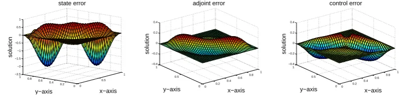
Figure 1. h= 2−6

√

2, τ = 4k/5, k∼=h4/3, t= 0.5: Errors for the state, adjoint and control errors.

6. Conclusion

We have shown that by balancing the errors, the convergence rates of the optimal solutions can be improved under SUPG discretization in space, which is common for OCPs, when the state, control and adjoint are discretized by linear finite elements. In case of higher order finite elements, for SUPG discretized diffusion-convection-reaction equations, the difference between the DO and OD is more significant. But this does not imply more accurate controls. This will be investigated in a future work for time-dependent diffusion-convection-reaction equations.

7. Acknowledgements

The authors wish to thank to Murat Uzunca for helpful discussions. This research was supported by the Middle East Technical University Research Fund Project (BAP-07-05-2012-102).

References

[1] Akman,T., Y¨ucel,H., and B. Karas¨ozen,B., (2013), A priori error analysis of the upwind symmetric interior penalty Galerkin (SIPG) method for the optimal control problems governed by unsteady convection diffusion equations, Comput. Optim. Appl., 57, pp.703-729.

[2] Akman,T. and Karas¨ozen,B., (2014), Variational Time Discretization Methods for Optimal Control Problems Governed by Diffusion- Convection-Reaction-Equations, Journal of Computational and Ap-plied Mathematics, 272, pp.41-56.

[3] Becker,R. and Vexler,B., (2007), Optimal control of the convection-diffusion equation using stabilized finite element methods, Numer. Math., 106, pp.349-367.

[4] Burman,E., (2011), Crank-Nicolson finite element methods using symmetric stabilization with an application to optimal control problems subject to transient advection-diffusion equations, Comm. Math Sci., 9, pp.319-329.

[6] Collis,S.S. and Heinkenschloss,M., (2002), Analysis of the streamline upwind/Petrov Galerkin method applied to the solution of optimal control problems. Tech. Rep. TR0201, Department of Computational and Applied Mathematics, Rice University, Houston, TX, 77005-1892.

[7] Ded`e,L., (2005), A. Quarteroni, Optimal control and numerical adaptivity for advection-diffusion equations. M2AN Math. Model. Numer. Anal., 39, pp.1019-1040.

[8] Douglas,Jr.J. and Russell,T.F., (1982), Numerical methods for convection-dominated diffusion prob-lems based on combining the method of characteristics with finite element or finite differences proce-dures. SIAM J. Numer. Anal., 19, pp.871-885.

[9] Fu,H., (2010), A characteristic finite element method for optimal control problems governed by convection-diffusion equations. J. Comput. Appl. Math., 235, pp.825-836.

[10] Fu,H. and Rui,H., (2009), A priori error estimates for optimal control problems governed by transient advection-diffusion equations. J. Sci. Comput., 38, pp.290-315.

[11] Hinze,M., Yan,N., and Zhou,Z., (2009), Variational discretization for optimal control governed by convection dominated diffusion equations. J. Comput. Math., 27, pp.237-253.

[12] John,V. and Novo,J., (2011), Error analysis of the SUPG finite element discretization of evolutionary convection-diffusion-reaction equations. SIAM J. Numer. Anal., 49, pp.1149-1176.

[13] Tr¨oltzsch,F., (2010), Optimal Control of Partial Differential Equations: Theory, Methods and Appli-cations, vol. 112 of Graduate Studies in Mathematics, American Mathematical Society, Providence. [14] Meidner,D. and Vexler,B., (2008), A priori error estimates for space-time finite element discretization

of parabolic optimal control problems. II. Problems with control constraints. SIAM J. Control Optim., 47, pp.1301-1329.

[15] Stoll,M. and Wathen,A., (2012), Preconditioning for partial differential equation constrained opti-mization with control constraints. Numer. Linear Algebra Appl., 19, pp.53-71.

[16] Stynes,M., (2005), Steady state convection-diffusion problems. Acta Numer., 14, pp.445-508. [17] Zhou,Z. and Yan,N. (2010), The local discontinuous Galerkin method for optimal control problem

governed by convection diffusion equations. Int. J. Numer. Anal. Model., 7, pp.681-699.

[18] Y¨ucel,Y. and Karas¨ozen,B., (2014), Adaptive Symmetric Interior Penalty Galerkin (SIPG) method for optimal control of convection diffusion equations with control constraints, Optimization, 63, pp.145-166.

Tugba Akman studied mathematics at Middle East Technical University(METU) in Ankara. She received her master degree in 2011 and PhD degree in 2015 from Scientific Computing Program at Institute of Applied Mathematics in METU. She worked for the Department of Mathematics in METU as a research assistant from 2009 to 2015. She joined the Department of International Trade & Finance in University of Turkish Aeronautical Association in 2016. Her research interests are optimal control problems, reduced-order modelling, sensitivity analysis, and error estimates of differential equations.

Bulent Karasozenfor the photography and short autobiography, see TWMS J. App. Eng. Math., V.1, N.2, 2011.