ISSN: 2008-6822 (electronic)
http://dx.doi.org/10.22075/ijnaa.2016.501
Projected non-stationary simultaneous iterative
methods
Touraj Nikazad∗, Mahdi Mirzapour
aSchool of of Mathematics, Iran University of Science and Technology, Tehran 16846-13114, Iran
(Communicated by M. Eshaghi)
Abstract
In this paper, we study Projected non-stationary Simultaneous Iterative Reconstruction Techniques (P-SIRT). Based on algorithmic operators, convergence result are adjusted with Opial’s Theorem. The advantages of P-SIRT are demonstrated on examples taken from tomographic imaging.
Keywords: simultaneous iterative reconstruction techniques; convex feasibility problem; (firmly) nonexpansive operator; cutter operator.
2010 MSC: Primary 65J22, 65J15; Secondary 65F10.
1. Introduction
Large-scale discretizations of ill-posed problems (as imaging problems in tomography) lead to large, sparse and ill-posed (sensitive to noise) linear systems of equations (which may be inconsistent) of the form
Ax=b. (1.1)
Many problems as image reconstruction [30, 12, 13, 26, 24, 23], computed tomography [21, 22, 34], image recovery [33, 35], image restoration [36], image registration [29], seismic imaging [20], image fusion [17], radar imaging [14] lead to a linear system as (1.1).
Finding x∗ ∈ Rn such that Ax∗ = b is a special case of convex feasibility problems (CFPs).
Actually many problems in mathematics and physical sciences can be modeled as a CFP, i.e., a problem of finding a point x∈Q=Tm
i=1Qi where {Qi} m
i=1 ⊆Rn are closed convex sets. Using fixed point iterative methods based on algorithmic operators has been suggested by many researchers for solving CFPs, see, e.g., [2, 8]. One of the most important class of algorithmic operators is
∗Corresponding author
Figure 1: ART method
projection algorithms that play a main role in the area of constructive solution of CFPs. Projection algorithms are iterative algorithms that use projections onto sets. We next give some instances of such algorithms.
Let A ∈ Rm×n and b ∈
Rm. Let ai and bi denote the i-row of A and b, respectively. Therefore
projection ofx∈Rn onto the i-hyperplane, i.e. H
i ={x∈Rn| hai, xi=bi}, is
PHi(x) = x+
bi− hai, xi kaik2 a
i
i= 1,2,· · · , m (1.2)
where i= 1,2,· · · , m. To simplifying the notation we denote PHi(x) =Pi(x).
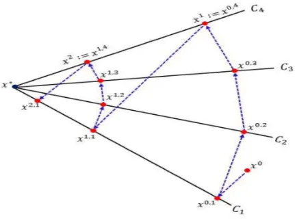
The projection operators can be used in various ways. We briefly explain a special case of sequential and simultaneous methods which use two different ways of projection operators. Algebraic Reconstruction Technique (ART) [21] is a sequential method which executes as follows. Let x0 ∈
Rn be an arbitrary starting point. The ART algorithm projects the current iteration xk onto a
hyperplane, e.g. Hi, and puts xk+1 =Pi(xk). Let T =Pm· · ·P2P1 where Pi is defined in (1.2). One
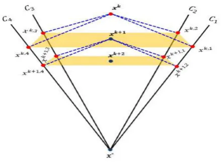
cycle of the ART method is performed by acting T on the staring point. In this way, we obtain a sequence of cycles which is a subsequence of iterations, see Figure 1. Simultaneous algorithms project xk onto all hyperplanes {Hi}mi=1 simultaneously. The next iteration is performed as convex combination of m new projected points, see Figure 2.
We now explain this algorithm with more details. Let T = Pm
i=1ωiPi, where
Pm
i=1ωi = 1 and
ωi ≥0.
Using (1.2) we get
T(x) =
m
X
i=1
ωiPi (1.3)
=
m
X
i=1
ωix+ωi
bi− hai, xi kaik2 a
i
=x+ATM(b−Ax) (1.4)
where
M =diag
ω1
ka1k2,· · · ,
ωm kamk2
Figure 2: Simultaneous method
Therefore, using (1.3) and (1.4), the fixed point iterative method xk+1 =T(xk) is a special case
of SIRT. In general, the SIRT is defined as the following iteration algorithm
xk+1 =xk+λkSATM b−Axk
k= 0,1,2, . . . (1.5)
where λk ∈[,2σ−2
1 ] are relaxation parameters and σ1 is the largest singular value of M 1 2AS
1
2. Also, M and S are assumed symmetric positive definite matrices. Several well-known fully simultaneous methods can be written in the form of (1.5) for appropriate choices of M and S matrices. We below give some instances
• Landweber’s method [28]: S =M =I,
• Cimmino’s method [15]: S =I and M = m1diagka1ik2
,
• CAV (Component Averaging method) method [? 12]: S = I and M = diag(1/Pn
j=1Nja2ij)
whereNj is the number of non-zeroes in the jth column of A,
• DROP (Diagonally Relaxed Orthogonal Projection) method [? ]: S = diag(m/Nj) and M any
symmetric positive definite matrix.
Furthermore, the SART method [1] and the symmetric Kaczmarz’s method [6] can be rewritten as (1.5).
When solving an inverse problem, the use of constraints (like nonnegativity) and prior information are well known techniques to improve the quality of the obtained solution because incorporate prior physical knowledge about the solution leads to smaller reconstruction errors, see [5, 4, 3, 7, 25, 32, 37]. In this paper we consider the projected version of equation (1.5) in a finite dimensional Euclidean space Rn. Let C ⊆ Rn denote a closed convex set and P
C be the metric projection onto C. Assume
that{λk}∞k=0 is a sequence of positive relaxation parameters. Now consider the following algorithm.
Algorithm 1.1. (P-SIRT)
Initialization: x0 ∈
Rn is arbitrary.
Iterative Step: given xk, compute
xk+1 =PC xk+λkSATM b−Axk
Definition 2.1. LetT :H →H and α∈[0,2]. The operator Tα defined by
Tα := (1−α)Id+αT (2.1)
is called an α-relaxation or, shortly, relaxation of the operator T. If α ∈ (0,2), then Tα is called a
strictly (or strict) relaxation ofT.
Definition 2.2. We say that an operator T :H →H is nonexpansive (NE), if
kT(x)−T(y)k ≤ kx−yk (2.2)
for all x, y ∈H. Also T is an α-contraction, where α∈(0,1) or, shortly, a contraction if
kT(x)−T(y)k ≤αkx−yk (2.3)
for all x, y ∈H.
Another useful class of operators is the class of cutter operators, namely
Definition 2.3. An operatorT :H →H with nonempty fixed point set is called cutter if
hx−T(x), z−T(x)i ≤0 (2.4)
for all x∈H and z ∈F ixT.
Remark 2.4. Based on [8, Remark 2.1.31] the operator T is a cutter if and only if
hT(x)−x, z−xi ≥ kT(x)−xk2 (2.5)
for all x∈H and z ∈F ixT.
Definition 2.5. We say that an operator T :H →H is firmly nonexpansive (FNE), if
hT(x)−T(y), x−yi ≥ kT(x)−T(y)k2 (2.6)
for all x, y ∈H.
Definition 2.6. LetT :H→H has a fixed point. Then the operator T is an α-relaxed cutter, or, shortly, relaxed cutter where α∈[0,2], if
hTα(x)−x, z−xi=αhT(x)−x, z−xi ≥ kT(x)−xk2 (2.7)
for all x∈H and z ∈F ixT. If α ∈(0,2), then Tα is called a strictly relaxed cutter operator of T.
Definition 2.7. Let α ≥ 0 and assume that T : H → H has a fixed point. We say that T is
α−strongly quasi-nonexpansive (α−SQNE), if
kT(x)−zk2 ≤ kx−zk2−αkT(x)−xk2 (2.8)
for all x ∈ H and z ∈ F ixT. Also, the operator T satisfying (2.8) with α > 0 is called strongly quasi-nonexpansive (SQNE) operator.
Following theorem presents the relationship between strictly relaxed cutter and SQNE operators.
Theorem 2.8. [8, Theorem 2.1.39 and Corollary 2.1.40] Assume that T :H →H has a fixed point and letλ ∈(0,2]. Then T is a λ-relaxed cutter if and only if T is 2−λλ-SQNE, i.e.,
kTλ(x)−zk2 ≤ kx−zk2−
2−λ
λ kTλ(x)−xk
2
(2.9)
for all x∈H and allz ∈F ixT.
Definition 2.9. An operator T :H →H is demi-closedat 0 if for any weakly converging sequence
xk* y ∈H with T(xk)→0 we have T(y) = 0.
Remark 2.10. It is well known, see [31, Lemma 2], the operatorT −Id is demi-closed at 0 where
T :H →H is a nonexpansive operator.
We now verify, using [9, Corollary 9.14.], that the sequence generated by Algorithm (1.1) con-verges.
Corollary 2.11. [9, Corollary 9.14.] and [8, Corollary 3.7.3] Let T : H → H be a cutter operator (e.g., a firmly nonexpansive operator having a fixed point) andx0 ∈H is an arbitrary point. Assume that the sequence {xk}∞
k=0 is generated by
xk+1 =PC xk+λk T(xk)−xk
for k = 1,2,· · · (2.10)
where λk∈(0,2).
(i) If lim infk→∞λk(2−λk)>0, then {xk}∞k=0 converges weakly to a fixed point of T.
(ii) If H is finite-dimensional andP∞k=0λk(2−λk) =∞, then {xk}∞k=0 converges to a fixed point of
T.
Let B = S12ATM AS 1
2 = (M 1 2AS
1 2)T(M
1 2AS
1
2) then the spectral radius of B is denoted by ρ(B) =σ2
1 where σ1 is the largest singular value of M
1 2AS
1
2. We next present a useful lemma from
Theorem 2.14. The sequence generated by Algorithm 1.1, where λk ∈ [, σ2 1
], converges to a solu-tion x∗ of minkAx−bkM.
Proof . Since λk ∈[,2σ−2
1 ] we can rewrite the Algorithm 1.1 as below
xk+1 =U(xk) =PC xk+
λk
ρ(S12ATM AS 1 2)
SATM(b−Axk)
!
(2.12)
=PC xk+λk T(xk)−xk
(2.13)
=PCTλk(x
k) (2.14)
where
T(x) = x+ 1
ρ(S12ATM AS 1 2)
SATM(b−Ax). (2.15)
Furthermore, we have
kT(x)−T(y)k=
(x−y)− 1
ρ(S12ATM AS 1 2)
SATM A(x−y)
=
I− 1
ρ(S12ATM AS 1 2)
SATM A
!
(x−y)
=
S12 I− 1
ρ(S12ATM AS 1 2)
S12ATM AS 1 2
!
S−21(x−y)
≤
S12 I− 1
ρ(S12ATM AS 1 2)
S12ATM AS 1 2
!
S−21
k(x−y)k
=
I− 1
ρ(S12ATM AS 1 2)
S12ATM AS 1 2 !
k(x−y)k.
Based on Lemma 2.12, Remark 2.13 and setting ¯A=S12A, we have
α =kI− 1
ρ( ¯ATMA¯)A¯ T
MA¯k= 1−σn2 <1.
consequently based on the first part of [8, Theorem 2.2.5] T is a cutter operator. Using Remark 2.10 we know that the operator T −I is demi-closed at 0. Therefore based on Corollary 2.11 the sequence {xk} converges weakly to a fixed point of T. Since we are using finite dimensional space
Rn we obtain xk →x∗ such that T(x∗) =x∗. It gives ATM(b−Ax∗) = 0 which is equivalent to the
fact thatx∗ is a minimizer of kAx−bkM.
3. Numerical Result
In this section we report some numerical results in field of medical imaging. Our numerical results show the effect of using projection operator after each iteration. Furthermore we suggest a rule for picking relaxation parameters.
In following two tables we show error histories for Landweber, Cimmino, CAV and DROP al-gorithms without constraint (C = Rn), with non-negativity constraints (C =
Rn+), and with box constraints (C = [0,1]n) within 40 iterations. For all of algorithms, we use the following strategy for
picking relaxation parameters that were proposed in [18, 19].
λk =
√
2σ1−2 for k = 0,1
2σ−12 1−ζk
(1−ζk k)2
, for k ≥0 (3.1)
where σ1 is largest singular value of M
1 2AS
1
2 and ζk are roots of a certain polynomial such that
0< ζk < ζk+1 and limk→∞ζk = 1.
The test is taken from the field of image reconstruction from projections using the SNARK93 soft-ware package [27]. We work with the standard head phantom from [21]. The phantom is discretized into 63×63 pixels, and 16 projections (evenly distributed between 0 and 174 degrees) with 99 rays per projection are used. The resulting matrix A has dimension 1584×3969, so that the system of equations is highly underdetermined. In addition toA, the software also produces a noise-free right-hand sidebsnark and a phantom (translated into vector form)x∗. Using SNARK93’s right-hand side
bsnark, which is not generated as the product Ax∗, we avoid committing an inverse crime where the
exact same model is used in the forward and reconstruction models. Apart from using noise-free data we also added additive independent Gaussian noise of mean 0 and relative noise-level (kδbk/kbsnarkk)
5% where bnoisy =bsnark+δb.
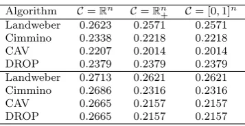
Table 1: The smallest relative error with noiseless (top) and noisy data (down) using Algorithm 1.1
Algorithm C=Rn C=Rn+ C= [0,1]n
Landweber 0.2623 0.2571 0.2571 Cimmino 0.2338 0.2218 0.2218 CAV 0.2207 0.2014 0.2014 DROP 0.2379 0.2379 0.2379 Landweber 0.2713 0.2621 0.2621 Cimmino 0.2686 0.2316 0.2316 CAV 0.2665 0.2157 0.2157 DROP 0.2665 0.2157 0.2157
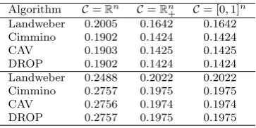
In Table 2, we demonstrate the effect of using this strategy.
Table 2: The smallest relative error with noiseless (top) and noisy data (down) using Algorithm 1.1 with relaxation parameters (3.2).
Algorithm C=Rn C=Rn+ C= [0,1]n
Landweber 0.2005 0.1642 0.1642 Cimmino 0.1902 0.1424 0.1424 CAV 0.1903 0.1425 0.1425 DROP 0.1902 0.1424 0.1424 Landweber 0.2488 0.2022 0.2022 Cimmino 0.2757 0.1975 0.1975 CAV 0.2756 0.1974 0.1974 DROP 0.2757 0.1975 0.1975
References
[1] A.H. Andersen and A.C. Kak,Simultaneous algebraic reconstruction technique (sart): a superior implementation of the art algorithm, Ultrason. imaging 6 (1984) 81–94.
[2] H.H. Bauschke and J.M. Borwein, On projection algorithms for solving convex feasibility problems, SIAM Rev. 38 (1996) 367–426.
[3] F. Benvenuto, R. Zanella, L. Zanni and M. Bertero,Nonnegative least-squares image deblurring: improved gradient projection approaches, Inverse Probl. 26 (2010): 025004.
[4] M. Bertero, D. Bindi, P. Boccacci, M. Cattaneo, C. Eva and V. Lanza, Application of the projected landweber method to the estimation of the source time function in seismology, Inverse Probl. 13 (1997): 465.
[5] M. Bertero and P. Boccacci,Introduction to inverse problems in imaging, CRC press, Florida, 1998.
[6] ˚A. Bj¨orck and T. Elfving, Accelerated projection methods for computing pseudoinverse solutions of systems of linear equations, BIT Numer. Math. 19 (1979) 145–163.
[7] P. Brianzi, F. Di Benedetto and C. Estatico,Improvement of space-invariant image deblurring by preconditioned landweber iterations, SIAM J. Sci. Comput. 30 (2008) 1430–1458.
[8] A. Cegielski,Iterative methods for fixed point problems in Hilbert spaces, Springer, Berlin, 2013.
[9] A. Cegielski and Y. Censor,Opial-type theorems and the common fixed point problem, In Fixed-Point Algorithms for Inverse Problems in Science and Engineering, Springer, New York, 2011, 155–183.
[10] Y. Censor and T. Elfving, Block-iterative algorithms with diagonally scaled oblique projections for the linear feasibility problem, SIAM J. Matrix Anal. Appl. 24 (2002) 40–58.
[11] Y. Censor, T. Elfving, G.T. Herman and T. Nikazad,On diagonally relaxed orthogonal projection methods, SIAM J. Sci. Comput. 30 (2008) 473–504.
[12] Y. Censor, R. Gordon and D. Gordon, Component averaging: An efficient iterative parallel algorithm for large and sparse unstructured problems, Parallel Comput. 27 (2001) 777–808.
[14] M. Cheney and B. Borden,Fundamentals of radar imaging, SIAM, Philadelphia, 2009.
[15] G. Cimmino and C.N. delle Ricerche,Calcolo approssimato per le soluzioni dei sistemi di equazioni lineari, Istituto per le applicazioni del calcolo, Fiorentino, 1938.
[16] L.T. Dos Santos,A parallel subgradient projections method for the convex feasibility problem, J. Comput. Appl. Math. 18 (1987) 307–320.
[17] M. Elad and A. Feuer,Restoration of a single superresolution image from several blurred, noisy, and undersampled measured images, IEEE Trans. Image Process. 6 (1997) 1646–1658.
[18] T. Elfving, P. Hansen and T. Nikazad,Semiconvergence and relaxation parameters for projected SIRT algorithms, SIAM J. Sci. Comput. 34 (2012) A2000–A2017.
[19] T. Elfving, T. Nikazad and P. Hansen,Semi-convergence and relaxation parameters for a class of SIRT algorithms Electron. Trans. Numer. Anal. 37 (2010) 321–336.
[20] H.W. Engl, A.K. Louis and W. Rundell,Inverse problems in geophysical applications, SIAM, Philadelphia, 1997. [21] G.T. Herman,Fundamentals of computerized tomography: image reconstruction from projections, Springer
Sci-ence, London, 2009.
[22] G.T. Herman and W. Chen,A fast algorithm for solving a linear feasibility problem with application to intensity-modulated radiation therapy, Linear Algebra Appl. 428 (2008) 1207–1217.
[23] M. Jiang and G. Wang, Development of iterative algorithms for image reconstruction, J. Xray Sci. Technol. 10 (2001) 77–86.
[24] M. Jiang and G. Wang,Convergence studies on iterative algorithms for image reconstruction, IEEE Trans. Med. Imag. 22 (2003) 569–579.
[25] B. Johansson, T. Elfving, V. Kozlov, Y. Censor, P. Forss´en and G. Granlund, The application of an oblique-projected Landweber method to a model of supervised learning, Math. Comput. Model. 43 (2006) 892–909. [26] A.C. Kak and M. Slaney,Principles of computerized tomographic imaging, SIAM, Philadelphia, 2001.
[27] J. Klukowska, R. Davidi, and G.T. Herman,SNARK09–A software package for reconstruction of 2D images from 1D projections, Comput. Methods Programs Biomed. 110 (2013) 424–440.
[28] L. Landweber,An iteration formula for Fredholm integral equations of the first kind, Amer. J. Math. 73 (1951) 615–624.
[29] J. Modersitzki,Numerical methods for image registration. Oxford university press, Oxford, 2003.
[30] F. Natterer and F. W¨ubbeling,Mathematical methods in image reconstruction, SIAM, Philadelphia, 2001. [31] Z. Opial, Weak convergence of the sequence of successive approximations for nonexpansive mappings, Bull. Am.
Math. Soc. 73 (1967) 591–597.
[32] M. Piana and M. Bertero,Projected landweber method and preconditioning, Inverse Probl. 13 (1997) 441–463. [33] A. Serbes and L. Durak,Optimum signal and image recovery by the method of alternating projections in fractional
fourier domains, Commun. Nonlinear Sci. Numer. Simul. 15 (2010) 675–689.
[34] K.T. Smith, D.C. Solmon and S.L. Wagner,Practical and mathematical aspects of the problem of reconstructing objects from radiographs, Bull. Am. Math. Soc. 83 (1977) 1227–1270.
[35] H. Stark and P. Oskoui, High-resolution image recovery from image-plane arrays, using convex projections. J. Opt. Soc. Amer. A. 6 (1989) 1715–1726.
[36] D.C. Youla, Generalized image restoration by the method of alternating orthogonal projections, IEEE Trans. Circuits Syst. 25 (1978) 694–702.