COMPLEXITY OF EMBEDDED CHAIN ALGORITHM FOR
COMPUTING STEADY STATE PROBABILITIES OF MARKOV CHAIN
Henrikas Pranevi
č
ius
Department of Business Informatics, Kaunas University of Technology Studentų St, 56-301, LT – 51368 Kaunas, Lithuania
e-mail: [email protected]
Eimutis Valakevi
č
ius, Mindaugas Šnipas
Department of Mathematical Research in Systems, Kaunas University of Technology Studentų St. 50-203, LT – 51368 Kaunas, Lithuania
e-mail: [email protected], [email protected]
Abstract. The paper presents the theoretical evaluation of the complexity of an algorithm, based on embedded
Markov chains, for computing steady state probabilities. Experimental research with different infinitesimal generator matrices was performed to support theoretical evaluations. Results showed that modified algorithm can be more effec-tive for sparse matrices. An example of a queuing system is presented to demonstrate the automatic creation of the model of the system based on the proposed modelling method.
Keywords: Steady state probabilities, complexity of the algorithm, numerical model, queuing system.
1. Introduction
The Markov chains are widely used for creating functioning models of various systems: computer net-works, communication systems, reliability models etc. It is known that the analytical solution of complex real world systems is very difficult or even impossible. Using numerical methods permits to model a wider class of systems. The process of creating numerical models for systems described by the Markov chain consists of the following stages:
1. Defining a state space of the Markov chain. 2. Generating a linear system of
Kolmogorov-Chap-man equations, describing the perforKolmogorov-Chap-mance of the system as a set of states and transitions among them.
3. Solving the linear system of Kolmogorov-Chapman equations, i.e., computing steady state probabi-lities.
4. Computing probabilistic characteristics of the system performance.
It is necessary to emphasize that automation is not equally applicable for all the stages. The first stage is determined in a heuristic way. The description of the system is the original that determines the state space of the system. The principal requirement in that stage
is to introduce a necessary number of coordinates to describe behavior of the system.
Most difficult stages in the construction of a nume-rical model are the creation and solution of the linear system of Kolmogorov-Chapman equations. The num-ber of equations is usually large (counted in thou-sands). Thus an automatic construction of linear systems and effective numerical solution methods are very important.
In order to demonstrate creation of numerical model we present an example of queuing system. There are a few different approaches to model queuing systems. In some cases, an exact solution of queuing systems can be found using the matrix geometric or the matrix analytical approaches [5, 8, 15]. Simulation (which in some aspects can be seen as opposite of analytical approach) is a powerful and universal scien-tific method to estimate the performance measures of various stochastic systems, including those based on queuing theory [1, 9]. One of the drawbacks of simulation is that sometimes it requires large amount of CPU time in order to achieve high accuracy. Vali-dation and verification of a model is also a difficult problem.
performance measures of queuing system. Such a numerical-analytical approach can be seen as a comp-romise among strictly analytical models and simula-tion, since it can achieve computational accuracy in relatively small amount of time.
In this paper we used the created software, which is based on Markov chains, to generate linear system of Kolmogorov-Chapman equations, which is stored in CPU memory as infinitesimal generator matrix of Markov chain. In book [14], the system that automates the construction of Markov models is presented. The embedded Markov chains are used for computing steady state probabilities of the Markov process. We used PLA formalism ([10, 13],etc.) to describe the performance of the system.
The former modeling and computation method was presented in [16] etc. In this paper we propose theoretical evaluation of the complexity of the algo-rithm. Theoretical results were compared with similar computation techniques and supported by experimen-tal results.
In the second section of the paper, the method of embedded Markov chains for computing steady state probabilities is presented. In the third section, we derive theoretical evaluation of the complexity of the algorithm for worst-case scenario. In Section 4, the modified algorithm for computing steady state prob-abilities is presented. It is proved that its slight modifycation improves the performance of the algorithm when infinitesimal generator matrix is sparse. In Section 5, an empirical research of the algo-rithm is presented. Experimental results with different infinitesimal generator matrices confirm theoretical evaluations of the complexity of the algorithm. An example of creating a numerical model of multi-class, multi-server queuing system is presented in the last section. In the paper, we use PLA formalism for description of the system performance and generation of Kolmogorov-Chapman equations [12].
2. An algorithm for computing steady state probabilities
Let PN
pijN NN be the transitions probabilitymatrix of the embedded Markov chain
x mN ,m0
N XN1 specified by . Let , ,,
be the sequence of the state spaces obtained by the following state space reduction routine:
} , , 2 iN
, {1
N i i
X X
1 X } , , , {1 2 k
k i i i
X ,
} / 1 1
k k
k X i
X , k1,N1.
Construct the sequence of Markov chains
x ,m0
,x( 1),m0
, , x1,m0
m N m N m
by em-bedding the chain
xmk,m0
into the chain
xmk1,m0
, k1,N1. It is proved that in thiscase the Markov chain
xm k,m0
is embedded into the chain
x mN ,m0
too. Since the Markov chain
0
1
N
P P1
P
,m
x n m
N
P
is specified by the and then we need to construct the sequence of transition mat-rixes , ,, . In [14], it is shown that the elements of matrixes , ,, are calculated according the formulas
n
P
N PN1
n X 1 P k k
p 1,i, 1 1 1 , 1 k k p 1 1 k 1 1 , 1 k
k i k ij p p k ij
p (1)
1 , 1 . ,
,kk
1
,j
i N
Steady state probabilities of discrete time Markov chain are calculated by the formulas
1 1 1 p ;
; 1 , ; 1 , 1 , , 1 1 1 N p p p k p k ii k j k ji k j k i 1 k 1,
k i
i
1
pki (2)
. , 1 ,j
1 ) ( ) ( ) ( N p p p N j N j N j N j
pj (3)
Formulas (1)-(3) are not convenient when dealing with practical problems. Usually, real systems are described by continuous time Markov chains. Therefore transitions are given as an infinitesimal generator matrix
N N
N ij
Q instead of the transi-tion probability matrix
N N N ij p N
P . To apply the algorithm to continuous time Markov chains, we substitute
ij p N j ij i i ij SS , 1
into (1). After the substitution we obtain the formulas , ) 1 ( , 1 k j k
) 1 ( 1 , ) 1 ( i k k i k ij S ) (k ij k j i, ; 1 N k N i j
ij, 1, 1,
, 1
S j i ) 1 ( 1 r .The non-normalized probabilities can be calculated recursively. At first we get
. 1
The other non-normalized probabilities are ( )
1 1
k i
r ( ) ( 1) 1
, 1, ,
, 1 1, 1.
k i N k k j ji j i
r i k
Finally, steady state probabilities qi,i
1,,N
are. , 1 ,
1 ) (
) (
N i r r
q N
j N j N i
i
3. Complexity analysis of the algorithm for calculating steady state probabilities
The worst-case scenario arises when all elements of the generator Q are non-zero. In this case, all elements of the matrix Q are stored in a two-dimension array. We will analyze two stages of the embedded chains algorithm separately.
The first stage of the algorithm is an embedding stage. The recalculated intensities are stored for the second step. The code is written in C++ and shown below:
void TForm1::EmbeddingStep(int n)
{
1 if ( n==2)
2 { M[0]=A[0][1];
3 sumn[0]=A[1][0]; }
4 else
5 { float sum = 0;
6 for (int i=0;i<(n-1);i++)
7 M[((n-1)*(n-1)-(n-1))/2+i]=Q[i][n-1] ;
8 for (int i=0;i<(n-1);i++)
9 sum = sum + Q[n-1][i];
10 sumn[n-2]=sum;
11 for ( int i=0;i<(n-1);i++)
12 for (int j = 0;j<(n-1);j++)
13 A[i][j]+=(Q[i][m-1]*Q[m-1][j]/sumn[n-2]);
14 EmbeddingStep(n-1);}
}
In order to evaluate the runtime complexity of the algorithm, we made a simplifying assumption, that different instructions (i.e. saving new variables, addi-tion, and multiplication) require equal amount of time, which we denote as 1. In steps 1-4, two variables are saved, so they require 2 units of time. While n > 2, steps 5-14 are executed recursively. Step 5 requires 1 unit of time. In steps 6-7 we have the loop, which is executed (n – 2) times, and each execution requires 1 unit of time. Analogically, in steps 8-9, the loop requires the same amount of time as in steps 6-7, and in step 10 one unit of time is required. In steps 11-13 we have the outer and inner loops which are executed (n – 1) times each. Since each execution requires 3 units of time, steps 11-13 require 3(n-1)² units of time in total.
We denote by the runtime complexity of the whole algorithm, and by and we denote the runtime complexity functions of the first and the second stages of the algorithm, respectively.
n T
nT1 T2
nIn order to find , we need to solve the inho-mogeneous difference equation of the first order
n
T
1
1
3
1
( 1))
( 2 1
1 n n n n T n
T
or
2 4 3 ) 1 ( )
( 2
1
1 n T n n n
T , nN (4)
with the seed value 2 ) 2 ( 1
T . (5)
The solution of a difference equation can be found by the method of undetermined coefficients. The characteristic polynomial is , so is a root having multiplicity 1. The general solution of homogenous part is
0 1
q q1
n c1 1 T
n c1TH n H , c1R. The particular solution has the form
2
2 1 0
0 n n p pnp n
, (6)
R p p
p0, 1, 2 .
To find coefficients , we substitute (3) into (1). We obtain the equation:
2 1 0,p,p p
2 2
0 1 2 2 1 3 2 3 2 3 4
p p p p n p n p n n n2. Comparing both sides, we have the system linear of equations
3 3
4 3 2
2
2 2 1
2 1 0
p p p
p p p
which has the solution
2 1 0
p ,
2 1 1
p , p2 1.
The general solution is the sum of the homogenous part and particular solution:
c n n n n
T
2 2 )
(
2 3
1 .
Constant c can be found from the seed value (2) 7
c .
The second stage of the algorithm is the calculation of steady state probabilities. The code in C++ is written below:
void TForm1::StacTik()
{
1 float r[n];
2 r[0]=1;
3 for ( int i=1; i<n; i++)
4 { r[i]=0;
5 for ( int j=0;j<i;j++)
6 r[i]+=r[j]*M[(i*i-i)/2+j];
7 r[i] = r[i]/sumn[i-1]; }
}
the running time of the second stage can be evaluated as follows:
1 1
2
1 0 1
2
2
( ) 2 2
1 2 ... ( 1) 2( 1) 2 2
2
1 3 2.
2 2
n i n
i j i
T n
n n
n n
n
n n
The complexity of the whole algorithm is equal to .
3 2 7 21 T n T n n n n
T
Eventually, using big O notation, the complexity of the algorithm is
n ~O
n3T . (7)
4. Complexity analysis of the modified algorithm
In the worst-case scenario, the algorithm has the run time complexity of O
n3 . Matrices which arise in practical problems (e.g. queuing networks) usually are very sparse. The algorithm of embedded chains can be modified for that case. Assuming that the matrix Q is not very large (i.e., it is possible to store the matrix in random access memory and no sparse matrix representation is necessary), steps 11-13 of the embedding stage of the algorithm can be written as follows:11 for ( int i=0;i<(n-1);i++)
12 if ( Q[i][n-1]>0)
13 {for (int j = 0;j<(n-1);j++)
14 Q[i][j]+=Q[i][n-1]*Q[n-1][j]/sumn[n-2]);}
In other words, we add an additional ‘if’ statement, in order to avoid superfluous instructions in step 14 of outer loop.
The run time complexity of the modified algorithm can be estimated using the recurrence relation. We denote by i – the number of nonzero entries in an
i-th column of i-the matrix Q, and is i
N
i
, , 1 max
.
The modified algorithm has one additional instruction in each outer loop, but the inner loop will be executed just ν times (at most). Obviously, until step 11, the modified algorithm requires the same amount of time (2(n-1)) as written in Section 3. ‘If’ statement in step 12 will be executed (n-1) times and steps 13-14 will be executed no more than ν(n-1) times (because of the modification), and each execution requires 3 units of time. The run time complexity can be expressed using the following recurrence relation:
1
1
3 ( 1) ( 1) 2)
( 1
1 n n n n T n
T
or
3 3
3 3) 1 ( )
( 1
1 n T n n
T , n,N
with seed value T(2)2.
The general solution of homogenous part is
n cTH , cR.
If n, or even, for example 10, the particular solution has the form
n n p0 p1n
0 ,
R p p0, 1 .
We can find using the method of undetermined coefficients. Again, we obtain the equation:
2 1 0,p,p p
3
3 32 1 1
0p pn n
p .
The values are the solution of the system of linear equations:
1 0,p p
. 3 2
3 3 1
1 0
p
p p
So
2 6 5 0
p ,
2 3 1
p .
In conclusion, the run time complexity of the embedding step of the modified algorithm is equal to
c n n
n
T
2 6 5 2
3 )
( 2
1 .
If we assume that
n
, then using big O notation, the complexity of the first stage is) ( ~ )
( 2
1 n O n
T .
(An exact value of the constant c can be found from the seed value, but it does not change the asymptotic evaluation).
Since the second step was not modified, we obtain the estimation of the run time complexity
2 21n T n ~ n
T n
T .
Therefore, for very sparse matrices, the modified embedded chains algorithm has the run time complexity of
n2 , which is better than classical Gaussian elimination. In addition, the run time comp-lexity of the embedded chains algorithm does not depend on the structure of the infinitesimal generator matrix Q.In order to compare the algorithms, we have used four different infinitesimal generator matrices of Mar-kov chains with 1000 000 elements each (i.e., matrices represent Markov chains with 1000 states). Since the matrices are relatively small, they were stored in two-dimension arrays.
For the first experiment we chose a Markov chain with all intensities among the states equal to 1 (i.e., matrix Q1 has all non-diagonal elements equal to 1). Obviously, in this trivial case the steady states prob-abilities are all equal to 0.001.
For the second experiment, we generated (i.e., using random number generator) infinitesimal gene-rator matrix Q05. Matrix Q05 was generated in such a way that all intensities among the states – i.e., non-diagonal elements of the matrix – are equal to 1 (with probability 0.5) or 0 (also with probability 0.5). We have also checked if the rank of the matrix Q is equal to (n-1). It is obvious that randomly generated matrix Q05 will have on average 50 % nonzero entries, and entries in matrix are scattered without any noticeable pattern or structure. In Figure 1 a portion of the matrix Q05 is shown.
Figure 1. Structure of matrix Q05
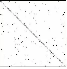
In the third experiment, we have generated matrix Q001 with the intensities among the states equal to 1 with probability 0.01, or 0 with probability 0.99. In this case, matrix Q001 will have on average 1 % nonzero entries (so it is a sparse matrix), and the entries again are scattered without any noticeable structure, except for diagonal (see Figure 2).
Figure 2. Structure of matrix Q001
For the last experiment, we use infinitesimal gene-rator matrix Q of the Markov chain, which describes a queuing system with quality control [14].
We have generated an infinitesimal generator matrix Q, using the created software, which is based on Markov chains. It generates the set of possible states, the generator and the steady state probabilities. In this case, the matrix Q is very sparse, nonsymmet-rical and highly structured ( Figure. 3).
Figure 3. Structure of matrix Q
Experimental run time analysis of algorithms was performed using a PC with AMD Athlon 64 X2 dual core processor 4000+ 2.10 GHz, 896 MB of RAM physical address extensions.
The experimental results are shown are in Table 1.
Table 1. Comparison of modeling results (time in seconds)
Generator
matrix Embedded chains embedded Modified chains
LU
decompo-sition
Q1 7.032 6.984 5.101
Q05 6.984 6.921 5.093
Q001 6.969 3.688 5.100
Q 6.969 0.047 5.095
Embedded chains algorithm is slightly less effec-tive than LU decomposition, if infinitesimal generator matrix is dense. However, if infinitesimal generator matrix is sparse (less than 1 percent non-zero entries) the modified algorithm outperforms LU decomposi-tion, and it is much more effective if infinetisimal generator matrix is very sparse.
6. Example: queuing system with Markov modulated service time
First In First Out (FIFO) manner. Server speed can change at service completion.
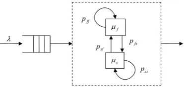
The system is represented schematically in Figure 4.
f s ss p ff p sf
p pfs
Figure 4. Scheme of the queuing system
Customers arrive into the queue according to a Poisson process with mean rate λ. Each arriving cus-tomer brings a certain amount of work distributed exponentially with mean which depends on some external Markov chain. In the following analysis we assume, that underlying Markov chain has two states, which we denote as slow S, and fast F. When the underlying Markov chain is in state S, server works at rate
s, and when Markov chain is in state F, server works at ratef. We assume that s f . If server is in state S and completes a service, it can remain in state S with probability , or it can transit in state F with probability . Similarly, if server is in state F, it can remain in the same state with probability , or it can transit in the state S with probability . ss p ss p 1 sf ff p 1 p ff p fs p Since customer arrival and service times have exponential distribution, performance of the whole queuing system can be described as Markov chain with infinitesimal generator matrix. There are a few different approaches to create infinitesimal generator matrix automatically. One can use tools based on Petri nets ([4, 6, 7]), stochastic automata networks forma-lism, proposed by Plateau ([2, 3, 11]) or other me-thods. In any case, the user must precisely describe the performance of the system.
We used the PLA formalism for numerical models [12] to describe the performance of the queuing system.
Aggregate specification of the queuing system is: 1. The set of input signals X = Ø.
2. The set of output signals Y = Ø. 3. The set of external events E' = Ø. 4. The set of internal events:
"
5 " 4 " 3 " 2 "
1, , , , " e e e e e
E ,
where – a customer arrived at the system; e1" "
2
e – a customer was served at state F and the state of the server did not change;
" 3
e – a customer was served at state F and the state of the server changed into S;
" 4
e – a customer was served at state S and the state of the server did not change;
" 5
e - a customer was served at state S and the state of the server changed into F.
5. The transition rates between states of the system: " 1 e s
e" 4
, , ,
, .
ff f p
e" 2
ss
p
e" 5
fs f
p
e
"
3sf sp
6. The discrete component of the state:
t
n1
t,n2 t
,
where n1
t – number of customers in the system;
tn2 – indicates the state of the server ( 0, if state is F and 1 if it’s S ).
7. The continuous component of the state:
t
w
e t we t we t we t we t
z 1", , "2, , "3, , "4, , 5", . 8. Initial state of the system:
t 0,0,,,,,
z .
9. Internal transition operators:
" 1H e : / a customer arrived at the system /
; , , , 1 0 1 1 11 n t otherwise L t n if t n t n
t
n
t n2 0 2 ;
e t
we t w 1", 0 1", ;
; , , 0 , 0 , 2 " 2 otherwise t n if p t ew f ff
; , , 0 , 0 , 2 " 3 otherwise t n if p t ew f fs
; , , 1 , 0 , 2 " 4 otherwise t n if p t ew s ss
. , , 1 , 0 , 2 " 5 otherwise t n if p t ew s sf
" 2 eH and H
e"5 :
0
1
1 1t n t n ;
0
0 2 t n ;
e t
we t w 1", 0 1", ;
; , , 1 , 0 , 1 " 2 otherwise t n if p t e
; ,
, 1 ,
0
, 1
" 3
otherwise t n if p t
e
w f fs
e"4,t0
w ;
e5",t0
w .
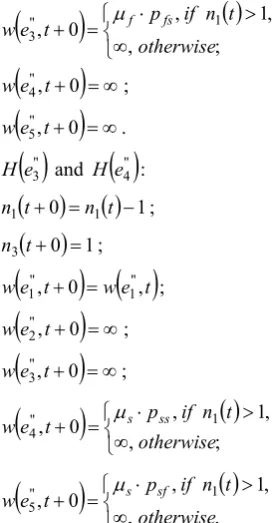
" 3 eH and H
e"4 :
0
1
1 1t n t n ;
0
1 3t n ;
e t
we t w 1", 0 1", ;
e"2,t0
w ;
e"3,t0
w ;
; ,
, 1 ,
0
, 1
"
4 otherwise
t n if p t
e
w s ss
. ,
, 1 ,
0
, 1
" 5
otherwise t n if p t
e
w s sf
The created software automatically builds infinite-simal generator matrix and estimates steady state probabilities
n1,n2
. System performance characte-ristics can be calculated using steady state probabi-lities. For example, loss probability (arriving customer finds L customers in the queue) is estimated by the formula
L
n n
n n L
P
1 2 2 1,
,
when waiting space is limited by L.
We modeled queuing systems with Markov modu-lated service times and with limitation on the waiting space (M/MMPP/1/N by Kendall notation). In order to compare run time of the modified algorithm with different size infinitesimal generator matrices, the limit imposed on the waiting space L was varied. Experimental results (in Table 2 and Figure 5) confirm theoretical complexity evaluation of the modified algorithm O(n²) , since run time of modified algorithm increases about 4 times, when the number of system states increases 2 times, and trend line is consistent with second order function.
Table 2. Computation time of the modified algorithm
Number of states CPU time, ms
600 16
800 31
1000 47
1200 62
1400 94
1600 141
Modeling results were compared with results ob-tained by analytical solution in [17]. Loss probability of the system with limited waiting space was
calculated when limitation on waiting space is 7. In Table 3 we can see that numeric modeling results coincide with results obtained analytically. The results were obtained with the software created in C++ program language.
0 20 40 60 80 100 120 140 160
0 500 1000 1500 2000
Number of states
ti
me
, ms
Figure 5. Computation time
Table 3. Comparison of numerical and analytical modeling
results
sf
p pfs P L( )an P L( )num
10
0.6 0.3 3.11% 3.11%
8
s
0.3 0.6 11.05% 11.05%
50
s
0.9 0.15 0.78% 0.78%
10
0.6 0.3 0.52% 0.52%
5 . 12
s
0.3 0.6 1.91% 1.91%
50
s
0.9 0.15 0.14% 0.14%
7. Conclusion
Embedded chains algorithm is designed specifi-cally for Markov chains. It is a direct algorithm, so theoretically it will calculate the exact solution in a finite number of steps. Theoretical analysis showed that the complexity of the embedded chains algortihm is O(n³) in the worst-case scenario, so it cannot out-perform Gaussian algortihm and its variants (LU de-composition) when infinetisimal generator matrix is dense. However, the modified algorithm becomes more effective when infinetisimal generator matrix is sparse. Theoretical and experimental results showed that the complexity of the modified algorithm is O(n²) when infinitesimal generator matrix is very sparse. References
[1] D. Bakšys, L. Sakalauskas. Simulation and testing of
FIFO clearing algortihms. Information Technology and Control, Vol. 39, No. 1,2010, 25-31.
[2] L. Brenner, P. Fernandes, B. Plateau, I. Sbeity.
PEPS2007 – Stochastic automata networks software tool. Fourth International Conference on the Quanti-tive Evaluation of Systems, QEST 2007, Edinburgh,
2007,163-164.
[4] K.S. Cheung. Refinement of Petri-net-based system specification. Information Technology and Control, Vol. 35, No. 2,2006, 137-143.
[5] M. Harchol-Balter, T. Osogami, A. Scheller-Wolf,
A. Wierman. Multi-server queueing systems with
multiple priority classes Queueing System, Vol. 51, 2005, 331-360.
[6] S. Kounev. Performance modelling and evaluation of
distributed component-based systems using queueing Petri nets. IEEE Transactions on Software Enginee-ring, Vol. 32, No. 7, 2006, 486-502.
[7] S. Kounev, C. Dutz. QPME: a performance modelling
tool besed on queueing Petri nets. ACM SIGMETRICS Performance Evaluation Review, Vol. 36, No. 4, 2009, 46-51.
[8] S.R. Mahabhashyam, N. Gautam. On queues with
Markov modulated service rates. Queueing Systems, Vol. 51,2005, 89-113.
[9] S. Minkevičius. Simulation of the open message
switching system. Information Technology and Control, Vol. 37, No. 1,2008, 75-78.
[10] Š. Packevičius, A. Kazla, H. Pranevičius. Extension
of PLA specification for dynamic system formalization. Information Technology and Control, Vol. 35, No. 3,2006, 235-242.
[11] B. Plateau, K. Atif. Stochastic automata network of
modeling parallel systems. IEEE Transactions on Soft-ware Engineering, Vol. 17, No. 10, 1991, 1093-1108.
[12] H. Pranevičius, V. Germanavičius, G. Tumelis.
Automatic Creation of Numerical Model of Systems Specified by PLA Method. 19th European Conference
of Modelling and Simulation, ASMTA 2005, 118-124.
[13] H. Pranevičius, A. Paulauskaitė-Tarasevičienė, D.
Makackas. Application of abstract data type in
dyna-mic PLA approach. Information Technology and Control, Vol. 38, No. 1,2009, 7-13.
[14] H. Pranevičius, E. Valakevičius. Numerical models
of systems specified by Markovian processes. Techno-logija, Kaunas, 1996.
[15] A. Sleptchenko, A. van Harten, M. van der Heij-den. An exact solution for the state probabilities of the multi-class, multi-server queue with preemptive prio-rities. Queueing Systems, Vol. 50, 2005, 81-107.
[16] E. Valakevičius, H. Pranevičius. An algorithm for
creating Markovian Models of Complex Systems,
Proceedings of the 12th World Multi-Conference on
Systemics, Cybernetics and Informatics, WSMCI 2008,
Orlando, 2008. 258-262.
[17] Y.P. Zhou, N. Gans. A Single-Server Queue with
Markov Modulated Service Times. Working paper, the Wharton School, University of Pensilvania.