Vol. 8, No. 1, 2016 Article ID IJIM-00431, 12 pages Research Article
A nonlinear model for common weights set identification in
network Data Envelopment Analysis
J. Pourmahmoud ∗†, Z. Zeynali ‡
Received Date: 2013-11-04 Revised Date: 2015-03-16 Accepted Date: 2015-12-03
——————————————————————————————–
Abstract
In the Data Envelopment Analysis (DEA) the efficiency of the units can be obtained by identifying the degree of the importance of the criteria (inputs-outputs).In DEA basic models, challenges are zero and unequal weights of the criteria when decision-making units are evaluated. One of the strategies applied to deal with these problems is using common weights of the each input/output in all decision making units (DMUs). In practice the DMUs are containing intermediate process. However, these units are considered as a black box in DEA basic models, disregarding internal process. This was the main reason network data envelopment analysis was introduced. On the other hand, similar challenges mentioned for DEA, zero and unequal weights of the criteria, exist for network structures as well. This paper suggests a common set of the weights for network structures to deal with the above problems using nonlinear models, for general case. Also some numerical examples using proposed models are presented.
Keywords : Network Data Envelopment Analysis (NDEA); Decision Making Units (DMU); Efficiency; Epsilon; Assurance Value.
——————————————————————————————–
1
Introduction
D
aduced by Charnes et al.[ta envelopment analysis (DEA), intro-1], is an im-portant tool for measuring the efficiency of decision making units (DMUs). This ba-sic model evaluate a set of unites in which∗Corresponding author e-mail adresses. [email protected]
†Department of Applied Mathematics, Azarbai-jan Shahid madani University, Tabriz, Iran.
‡Department of Applied Mathematics, Azarbai-jan Shahid madani University, Tabriz, Iran.
similar inputs applied to produce similar outputs. This method allocates weights to both input and output indicators to max-imize the relative efficiency of each evalu-ated unit. The determined weights for each indicator are calculated in the best form for all the DMUs, in which they may vary from unit to unit. Charnes et al. classified set of controls on weights as following:
i) Direct analysis rejecting or assuming zero weight and eliminating some factors (ε). ii) Ignoring decision maker’s ideas.
iii) Considering a relative importance of some factors by decision maker.
iv) Discarding the number of DMUs when the number of indicators is more than the number of DMUs under evaluation.
The common weights approach in DEA, initially introduced in 1990 by Cook et al.[3], and Roll et al.[4] in 1991, is known as one of the accurate approaches for evaluat-ing all DMUs considerevaluat-ing a unique weights for all the DMUs. Other researchers adopted some of the strategies for reaching common set of the weights. For instance, Roll et al.[4] obtained the common weights by narrowing the range of the weights and reducing domain using weighted average of the weights ¯Ur =
∑
jEjurj
∑
jEj and ¯Vi =
∑
jEjvij
∑
jEj , in which Ej is the efficiency of
DM Uj. In 1995, Doyle [5] considered the
optimized average weights of all DMUs as the common weights. In 2013, Hossein-zadeh et al.[6] used multi-objective pro-gramming (MOP) method to attain the common weights. In 2005, Kao and Hung [7] proposed the best common weights for the two-stage network model using the cal-culated efficiency scores of DEA model and the shortest distance function.
Usually in the evaluating DMUs there are internal process with their own input and outputs. In some cases an internal output can be an input for another internal process or it can be the main output of the unit. In these system the output may get affected by the internal process and ignoring these internal process will result on inaccurate outcome. For the first time, in 1996, Fre and Grosskopf [8] called these units as net-worked structure units.
Network structures are generally clas-sified into series, parallel, and general groups.The structures or units in which the internal processes are connected in series mode, known as a series network model. Kao and Hwangs, in 2008 [9], Fukuyama and Webers in 2010 [10], and Tone and
2
Review of the literature
In this section the common weight model based on Kaos multiple network model ap-proach [12] and Hosseinzadeh et al. [6] is presented.
2.1 obtaining common weight
us-ing MOP
Hosseinzadeh et al.(2013), [6] evaluated ef-ficiency of the DMUs by common weights and using MOP. MOP method is an opti-mization process for two or more possibly conflicting optimization processes and sub-jected to certain restrictions.
Suppose that J number of the DMUs consume m input DMU to produce s out-put. The following MOF problem gives the maximum simultaneous efficiency of the all DMUs:
M ax { ∑s
r=1uryrj
∑m
i=1viyij |j= 1,2,· · ·, J}
s.t. ∑s
r=1uryrj
∑m
i=1viyij ≤1; ∀j
ur ≥ε; ∀r
vi≥ε; ∀i
(2.1) There are several approach for solving problem (2.1). Goal programming is one of the main methods of the MOP [15]. In goal programming approach, decision maker consider all ideal levels for objec-tive functions. Hence, the sum of the de-viations from ideal levels, as the objec-tive function of goal programming problem will be minimized. Accordingly, if Aj, j =
1,2,· · ·, J, presents the goal of the jth ob-jective function and φ+j , φ−j are negative deviation (under-achievement) and positive deviation (over-achievement)of the jth goal, respectively, Model (2.1) can be written as follows:
min ∑Jj=1φ−j +φ+j s.t.
∑s r=1uryrj ∑m
i=1vixij +φ
− j −φ
+
j =Aj; ∀j (a) ∑s
r=1uryrj ∑m
i=1vixij ≤1; ∀j (b)
ur≥ε; ∀r
vi≥ε; ∀i
(2.2)
On the other hand, according to constraint (2.2 b), the positive deviation (φ+j) lacks a positive value and as a result, φ+j = 0. Thus, this Constraint (2.2b) is redundant and the constraint (2.2a), consideringAj =
1, can be written as follows:
s
∑
r=1
uryrj+φ−j m
∑
i=1
vixij = m
∑
i=1
vixij ∀j
(2.2-1) Thus, the non-linear model (2.2-1) cannot be transformed into a linear form. There-fore, Hosseinzadeh et al., for linearization of Model (2.2) using the concept of goal programming and substituting Aj = 1 in
Model (2.2), presented the following model to obtain the common set of weights:
min
J
∑
j=1 φj
s.t.
s
∑
r=1
uryrj− m
∑
i=1
viyij +φj = 0 ∀j
ur, vi ≥ε, ∀r, i
φj ≥0, ∀j
(2.2-2) in which φj is the deviation from goal
(unity value for the efficiency score). Using this model, the common set of weights for a set of DMUs under evalua-tion is obtained and the units utilizing ob-tained common set of the weights are eval-uated. However, when this model has mul-tiple optimal solutions, ranking units may vary. This is considered a drawback for Hosseinzadeh et al. study and this paper suggests strategies to avoid this issue.
2.2 NDEA multiplier models
provided a methodology to convert the sys-tem with an overall network structure to a series network structure while each struc-ture has parallel strucstruc-ture (s).
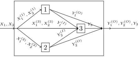
Kazemi Matin and Azizi [16] in 2015 in-troduced the integrated NDEA model to measure the production systems perfor-mance and showed that the model pre-sented by Kao (2009), is a special case of the presented model. Kao introduced a general network structure using an example in which each unit had the third divisions (Figure1).
In Kao example, system main inputs and outputs are X1 and X2 and Y1,Y2 and Y3, respectively. Division 1 may consumes only some ofX1 andX2 values for producingY1 and a part ofY1may remains for division 3. Division 2 consumes a specific value of X1 and X2 producing Y2 similar to division 1 and a part of Y2 for division 3. Division 3 consumes the rest of X1 and X2 alongside with the parts producedY1andY2resulting from divisions 1 and 2 for producing Y3.
Assume thatXij(k) indicates theith input of divisionk(k= 1,2,3) fromDM Uj.
Par-ticularly, sum of all inputs of three divisions (Xij(1) +Xij(2)+Xij(3)) for system input are Xij(j = 1,· · ·, J, i = 1,2). It means that
(Xij(1)+Xij(2)+Xij(3)) =Xij; i= 1,2,
j = 1,· · ·, J.
The output of division 1 is separated as Y1(I), Y1(O), where, Y1(O) is the system final output andY1(I)is a value consumed by the division 3 as an input. Similarly, output of division 2 is Y2(I), Y2(O), where Y2(o) is the system final output andY2(I)is a value con-sumed by division 3 as an input. Accord-ingly,
Yrj(I)+Yrj(O)=Yrj; r= 1,2;
j= 1,· · ·, J.
Multiplier model of general network
structure of figure1 is as follows:
Eo : f or o= 1,· · ·, J
M ax u1y1(oo)+u2y2(oo)+u3y3o
s.t. v1x1o+v21x2o = 1
(u1y(1oj)+u2y2(oj)+u3y3j)
−(v1x1j+v2x2j)≤0 ∀j
u1y1j−(v1x(1)1j +v2x(1)2j)≤0 ∀j
u2y2j−(v1x(2)1j +v2x(2)2j)≤0 ∀j
u1y3j−(v1x(3)1j +v2x(3)2j
+u1y1(Ij)+u2y2(Ij))≤0 ∀j
u1, u2, u3, v1, v2,≥ε
(2.3) Where, ur indicates the allocated weight
to rth output (r = 1,2,3) and vi is the
allocated weight to theith input (i= 1,2) used for measuring system efficiencyDM Uo
of the each process. As observed in model
2.3, X1 input weight is always v1 no mat-ter to be used by division 1 for x(1)1j input,
division 2 as x(2)1j or division 3 as x(3)1j ; or thaty1 output weight is alwaysu1 no mat-ter to be used by division 3 as input or to be the final output of the system. Other indices complies in a similar condition.
..
1
.
2
. 3
.
X1, X2
. X
(3) 1 , X
(3) 2 .
X (1)
1 , X
(1) 2
.
X(2) 1
, X(2) 2
. Y1(I) .
Y(
I) 2
. Y3
.
Y1(O) .
Y(O
) 2
. Y
(O) 1 , Y
(O) 2 , Y3
Figure 1: A network system with three division.
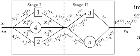
Kao also showed that every general net-work structure could be converted into a two-stage network structure through intro-ducing dummy divisions, where each stage has a parallel structure. If dummy divi-sions 4 and 5 are added in Figure 1 as an example, Figure 2 with two-stage parallel structure will be created.
fol-.. 1 . 2 . 4 . 3 . 5 . Stage I . Stage II .
X.1
X2
. X
(3) 1 .
X2(3)
. X (1) 1 , X (1) 2 . X(2) 1 , X
(2) 2 .
Y(O)
1
, Y1(I) .
Y(
O)
2
, Y
(I)
2
. X
(3) 1 .
X(3)2
. X (3) 1 , X (3) 2 . Y (I) 1
, Y (I)
2 .
Y1(O)
, Y2(O)
.
Y
3 .
Y
(O)
1
, Y
(O)
2
. Y
(O) 1 , Y
(O) 2 .
Y3
Figure 2: An equivalent tandem system where each stage
has a parallel structure.
lowing.
Eo(1) = u
∗ 1y1o
v1∗x(1)1o+v2∗x(1)2o
Eo(2) = u
∗ 2y2o
v1∗x(2)1o+v2∗x(2)2o
Eo(3) = u
∗ 3y3o
v1∗x(3)1o+v2∗x(3)2o+u∗1y(1Io)+u∗2y2(Io)
(2.4)
The efficiency score of the two stages shown in Figure 2, can be obtained using following relation.
EI o =
u∗1y1o+(v∗1x (3) 1o+v∗2x
(3) 2o)+u∗2y2o
v∗1x1o+v∗2x2o
EII
o =
u∗1y (o) 1o+u∗2y
(o) 2o+u∗3y3o
u∗1y1o+(v1∗x(3)1o+v∗2x(3)2o)+u∗2y2o
(2.5)
So that according to 2.5, the overall ef-ficiency is equal to the product efef-ficiency of the two stages, in other words: Eo =
EoI×EoII
3
Common weights in
network structures
3.1 Common weights considering
units efficiency deviation
Suppose J is the number of the network structures and each structure consist of K divisions (K=3 for the Kao example). Each division can receive input(s) from the out-side or from other division(s), consuming them in production process to generate the main output of the system. The generated output also can be received by the another division of the system.
For Kao’s network structure a model is introduced to obtain the common weights set.
min ∑Jj=1φj
s.t. (u1y1(oj)+u2y(2oj)+u3y3j)
−(v1x1j+v2x2j) +φj = 0 ;∀j
u1y1j−(v1x(1)1j +v2x
(1)
2j )≤0 ;∀j
u2y2j−(v1x(2)1j +v2x(2)2j )≤0 ;∀j
u3y3j−(v1x(3)1j +v2x(3)2j
+u1y1(Ij)+u2y(2Ij))≤0 ;∀j
u1, u2, u3, v1, v2≥ε ∀j
φj ≥0 ∀j
(3.6) Where φj is the efficiency deviation of
DM Uj and u1, u2, u3, v1, v2 are the com-mon weight indicators. In this model the goal is to minimize the sum of φj, subject
to maximizing the efficiency scores of the network structure and divisions.
If (v∗r, u∗i) is the optimal solution, the effi-ciency score forDM Uj is calculated as
fol-lows:
Ej∗= ∑s
r=1u∗ryrj
∑m
i=1u∗ixij (3.7)
The units can be ranked using obtained efficiency scores from equation (3.7).
When a problem has multiple optimal solutions, the objection of ”the ranking is not stable” is appeared. Thus, in order to resolve the objection, the problem is con-verted into a two-phase problem, in which the first phase is solving the Model (3.6), and the second is solving following model:
M ax min {(u1y (O)
1j +u2y2(Oj)+u3y3j)
(v1x1j+v2x2j) |∀j}
s.t. (u1y (O) 1j +u2y
(O)
2j +u3y3j)
−(v1x1j+v2x2j) +φ∗j = 0 ∀j
u1y1j−(v1x (1) 1j +v2x
(1)
2j )≤0 ∀j
u2y2j−(v1x (2) 1j +v2x
(2)
2j )≤0 ∀j
u3y3j−(v1x (3) 1j +v2x
(3) 2j
+u1y (I) 1j +u2y
(I)
2j )≤0 ∀j
u1, u2, u3, v1, v2≥ε
Variable
λ=min{u1y
(O)
1j +u2y(2Oj)+u3y3j
v1x1j+v2x2j |∀j}
is defined to change the multi-objective model (3.8) into the nonlinear model as fol-lows:
M ax λ
s.t. u1y
(O) 1j +u2y
(O) 2j +u3y3j
v1x1j+v2x2j ≥λ
(u1y1(Oj)+u2y(2Oj)+u3y3j)
−(v1x1j+v2x2j) +φ∗j = 0 ∀j
u1y1j−(v1x(1)1j +v2x(1)2j )≤0 ∀j
u2y2j−(v1x(2)1j +v2x(2)2j )≤0 ∀j
u3y3j−(v1x(3)1j +v2x(3)2j
+u1y1(Ij)+u2y2(Ij))≤0 ∀j
u1, u2, u3, v1, v2, λ≥ε
(3.9)
By solving the nonlinear model (3.9 ) and obtaining the weights, (v∗r, u∗i), the effi-ciency score ofDM Ujis calculated as (3.7).
In Model (5),
(v1, v2, u1, u2, u3, φ) = (0,0,0,0,0,0)
satisfies in the first four constrains, and considering the fifth constrains and the ob-jective function in the optimum solution the weights reaches into near zero.
Because of the computer limited memory, answers are strongly depend on the value of epsilon; and sometimes irrational results on obtaining error propagation. Therefore, to resolve with this problem, the epsilon has to be obtained from [17] and the optimum
value is used in Models (3.6) to (3.12 ).
M ax ε
s.t. v1x1j+v2x2j ≤1 ∀j
(u1y (o) 1j +u2y
(o)
2j +u3y3j)
−(v1x1j+v2x2j)≤0 ∀j
u1y1j−(v1x (1) 1j +v2x
(1)
2j)≤0 ∀j
u2y2j−(v1x (2) 1j +v2x
(2)
2j)≤0 ∀j
u3y3j−(v1x (3) 1j +v2x
(3) 2j
+u1y (I) 1j +u2y
(I)
2j )≤0 ∀j
u1−ε≥0 u2−ε≥0 u3−ε≥0 v1−ε≥0 v2−ε≥0
(3.10) For example, if the optimum value for the Model (3.10) is ε∗, the Model (3.6 ) con-straint Type 5 is as follows:
u1, u2, u3, v1, v2 ≥ε∗, φj ≥0 ∀j
Usingε∗ in other models is alike.
Model (3.10) is used for finding ε∗ . ε∗ is used for finding, divisions, stage, and over-all efficiency of the system. It should be noted that the obtained values for the effi-ciency usingε∗ may vary slightly with the values obtained using Kaoa’s model.
3.2 Common weights of network
structures with efficiency de-viation of the units and divi-sions
conditions the model is as follows:
min ∑Jj=1(φj+
∑3
k=1φkj) s.t. (u1y
(o) 1j +u2y
(o)
2j +u3y3j) −(v1x1j+v2x2j) +φj= 0
u1y1j−(v1x (1) 1j +v2x
(1)
2j) +φ1j= 0
u2y2j−(v1x (2) 1j +v2x
(2)
2j) +φ2j= 0
u3y3j−(v1x (3) 1j +v2x
(3) 2j
+u1y (I) 1j +u2y
(I)
2j ) +φ3j= 0
j= 1,2,· · ·, J φj, φkj≥0; ∀k, j
u1, u2, u3, v1, v2≥ε∗
(3.11)
By solving this model, the common weights set of the system units under eval-uation is achieved using the maximum effi-ciency of units and divisions.
Suppose (vr∗, u∗i, φ∗j, φ∗kj) is the optimal solution of model (3.11), the efficiency score ofDM Uj is obtained using the relationship
as (3.7). Hence, the DMUs can be ranked based on the obtained efficiency scores.
However, when the problem has multiple optimal solutions, the ranking of the DMUs will be unstable. To resolve this objection, a two-phase model has to be solved. The first phase of model is (3.11) and the second phase of the model is as follows:
M ax min {u1y (O)
1j +u2y2(jO)+u3y3j v1x1j+v2x2j |∀j}
s.t. (u1y (O) 1j +u2y
(O)
2j +u3y3j) −(v1x1j+v2x2j) +φ∗j = 0
u1y1j−(v1x (1) 1j +v2x
(1)
2j) +φ∗1j= 0
u2y2j−(v1x (2) 1j +v2x
(2)
2j) +φ∗2j= 0
u3y3j−(v1x (3) 1j +v2x
(3) 2j
+u1y (I) 1j +u2y
(I)
2j ) +φ∗3j = 0
j= 1,2,· · ·, J u1, u2, u3, v1, v2≥ε∗
(3.12) The multi-objective model (3.12) is trans-ferred to the model (3.13) by introducing the below variable
λ=min{u1y
(O)
1j +u2y(2jO)+u3y3j
v1x1j+v2x2j |∀j}
M ax λ
s.t. u1y (O)
1j +u2y(2jO)+u3y3j v1x1j+v2x2j ≥λ
(u1y (O) 1j +u2y
(O)
2j +u3y3j)
−(v1x1j+v2x2j) +φ∗j = 0 ∀j
u1y1j−(v1x (1) 1j +v2x
(1)
2j)φ∗1j= 0 ∀j
u2y2j−(v1x (2) 1j +v2x
(2)
2j)φ∗2j= 0 ∀j
u3y3j−(v1x (3) 1j +v2x
(3) 2j
+u1y (I) 1j +u2y
(I)
2j)φ∗3j= 0 ∀j
u1, u2, u3, v1, v2, λ≥ε∗
(3.13)
The efficiency scores is obtained by sub-stituting the presented model results in equation (3.7). Using obtained scores DMUs are ranked, and the challenge of zero weights is eliminated.
4
Numerical example
To demonstrate performance of the proposed models, the models are investi-gated considering two examples of Kao in [9] and [12]. The first is a simple example including five decision-making units A, B, C, D, E, with three intermediate divisions as its structure is shown in the Figure 1. The second example is a case study intro-duced by Kao about Twenty four Non-life insurance companies in Taiwan. He con-sidered these companies as decision making units (system), each consisting two inter-mediate divisions.
Example 4.1. Consider five
decision-making units A, B, C, D, E, each consist-ing three Divisions. The structure of each decision-making unit is shown in Figure 1. The inputs/outputs of all the systems are listed in Table 1.
Table 1: Input/output data of Kao example in the Year 2009.
DMU P X1 X2 y1(o) y (I) 1 y
(o) 2 y
(I) 2 y3
A 11 14 2 - 2 - 1
1 3 5 2 2 - -
-2 4 3 - - 2 1
-3 4 6 - 2 - 1 1
B 7 7 1 - 1 - 1
1 2 3 1 1 - -
-2 2 1 - - 1 1
-3 3 3 - 1 - 1 1
C 11 14 1 - 1 - 2
1 3 4 1 1 - -
-2 5 3 - - 1 1
-3 3 7 - 1 - 1 2
D 14 14 2 - 3 - 1
1 4 6 2 1 - -
-2 5 5 - - 3 1
-3 5 3 - 1 - 1 1
E 14 15 3 - 2 - 3
1 5 6 3 1 - -
-2 5 4 - - 2 2
-3 4 5 - 1 - 2 3
Thus, the overall assurance interval is (0,0.0344828]. Table2shows the values for the traditional CCR model, and Kao model (3.9) in two modes, without value and with overall assurance value, and CSW model.
Table 2: Comparing 5 DMU system perfor-mances independently calculated through ordi-nary model CCR, Kao model and the model presented here.
DMU E-CCR E-CCRε EN-CCR ENε EN-CSW A 1.0000 0.9266 0.5227 0.4744 04667 B 0.8980 0.8832 0.5952 0.5895 0.5833 C 0.8485 0.7377 0.5682 0.5209 0.5133 D 1.0000 1.0000 0.4821 0.4706 0.4702 E 1.0000 1.0000 0.8000 0.7931 0.7931
As it is shown in the table 2, applying a common set of the weights, DM UA and
DM UD rankings are replaced comparing
with the rank obtained from Kao network structure efficiency scores . And this re-placement is due to applying the common weights for evaluating the units. Further-more, considering calculation of epsilon us-ing Toloos model, values are obtained for CCR efficiencies and network model are slightly different from Kaos solution [?]. For instance, in Kao CCR model, DM UA
efficiency value is 1 regarded as an efficient unit. But, with using the epsilon obtained equal to 0.9266, it is considered as an inef-ficient unit.
As Table 2 shows, using εassurance value in CCR model, Unit A is converted from ef-ficient state to inefef-ficient state, and the effi-ciency scores of units C,and B are dropped. In addition, using the assurance value εin NDEA-CCR model, the efficiency scores of all the units are reduced; though, ranking of the units are still constant.
The Weights obtained from Kao’s model and CSW proposed model are given in Ta-ble3.
Table 3: The weights of the five DMUs calcu-lated independently via Kaos model, and CSW proposed model
DMU v1 v2 w1 w2 u3
A 0.0470 0.0345 0.0784 0.0643 0.1891 B 0.0345 0.1085 0.1613 0.0888 0.3395 C 0.0470 0.0345 0.0784 0.0643 0.1891 D 0.0369 0.0345 0.0708 0.0542 0.1665 E 0.0345 0.0345 0.0690 0.0517 0.1609 CSW 0.0345 0.0345 0.0690 0.0517 0.1609
In the above table, Rows 2 to 6 are the weights obtained from Kao network struc-ture model and the last row is the common set of the weights obtained using set of common weight model. The efficiency of stages and divisions of 5 evaluation units considering Kao models and common weight set are presented in the following table.
Table 4: Efficiency scores processes and stages calculated from the Kaos network model
DMU P.eff.Kao S.eff.Kao
E1 E2 E3 ES1 ES2
A 1.0000 0.6613 0.3070 0.9013 0.5264 B 0.8188 1.0000 0.5003 0.9286 0.6348 C 0.5618 0.3796 0.7204 0.6677 0.7801 D 0.5990 0.6069 0.4029 0.7174 0.6561 E 0.7273 0.6667 1.0000 0.7931 1.0000
Table 5: Efficiency scores processes and stages calculated from the CSW proposed model
DMU P.eff.CSW S.eff.CSW
E1 E2 E3 ES1 ES2
A 1.0000 0.6429 0.3011 0.9000 0.5185 B 0.8000 1.0000 0.4912 0.9286 0.6282 C 0.5714 0.3750 0.6914 0.6800 0.7549 D 0.6000 0.6000 0.4058 0.7143 0.6583 E 0.7273 0.6667 1.0000 0.7931 1.0000
Example 4.2. Consider the example
of 24 Taiwanese insurance companies ex-tracted from Kao and Hwang paper 2.4 in which the structure of each is similar to Figure 3. Inputs/outputs of the insurance companies are listed in Table 3.
..
1
. 2
.
X1, X2
. X2
.
X1 .
Z
1, Z 2 .
Y1
. Y2
.
Y1, Y2
Figure 3: Network structure of the insurance operation system.
Table 6: Input/output table of Kao, case study: Taiwanese insurance companies in 2008. DMU X1 X2 Z1 Z2 Y1 Y2 DM U1 1178744 673512 7451757 856735 984143 681687
DM U2 1381822 1352755 10020274 1812894 1228502 834754
DM U3 1177994 592790 4776548 560244 293613 658428
DM U4 601320 594259 3174851 371863 248709 177331
DM U5 6699063 3531614 37392862 1753794 7851229 3925272 DM U6 2627707 668363 9747908 952326 1713598 415058
DM U7 1942833 1443100 10685457 643412 2239593 439039
DM U8 3789001 1873530 17267266 1134600 3899530 622868 DM U9 1567746 950432 11473162 546337 1043778 264098
DM U10 1303249 1298470 8210389 504528 1697941 554806
DM U11 1962448 672414 7222378 643178 1486014 18259
DM U12 2592790 650952 9434406 1118489 1574191 909295
DM U13 2609941 1368802 13921464 811343 3609236 223047
DM U14 1396002 988888 7396396 465509 1401200 332283
DM U15 2184944 651063 10422297 749893 3355197 555482
DM U16 1211716 415071 5606013 402881 854054 197947 DM U17 1453797 1085019 7695461 342489 3144484 371984
DM U18 757515 547997 3631484 995620 692731 163927
DM U19 159422 182338 1141950 483291 519121 46857 DM U20 145442 53518 316829 131920 355624 26537
DM U21 84171 26224 225888 40542 51950 6491
DM U22 15993 10502 52063 14574 82141 4181
DM U23 54693 28408 245910 49864 0.1 18980
DM U24 163297 235094 476419 644816 142370 16976
Implementing Toloo model using the data in Table 3 results on the overall assurance intervalε∗∗= 1.04573e−8. Thus, the over-all assurance interval is (0,1.04573e−8]. Kao implementation results are listed in Tables 4and 5in the following two states: 1. Without any value;
2. With overall assurance value
In this table, the second, third, fourth and sixth columns are the results of implement-ing traditional CCR −ε models without overall assurance value, traditionalCCR−ε with overall assurance value, network with-out an overall assurance value, and network with the overall assurance value obtained from model NDEA-PZ, respectively. The fifth and seventh columns are units rank-ings in network models without overall as-surance value and with overall asas-surance value respectively.
Table 7: Comparing the efficiencies of 24 insurance companies in Taiwan independently calculated through ordinary CCR model and Kao model.
DMU E-CCR E-CCR-ε EN-Kao R-Kao
DM U1 0.984 0.978 0.996 4
DM U2 1.000 1.000 1.000 1.5
DM U3 0.988 0.970 0.936 5
DM U4 0.488 0.488 0.488 11
DM U5 1.000 1.000 0.979 3
DM U6 0.594 0.588 0.390 15
DM U7 0.470 0.467 0.374 17
DM U8 0.415 0.415 0.295 20
DM U9 0.327 0.327 0.280 22
DM U10 0.781 0.772 0.705 9
DM U11 0.283 0.277 0.283 21
DM U12 1.000 1.000 0.714 8
DM U13 0.353 0.351 0.337 18
DM U14 0.470 0.468 0.394 14
DM U15 0.979 0.972 0.737 7
DM U16 0.472 0.472 0.321 19
DM U17 0.635 0.633 0.427 13
DM U18 0.427 0.426 0.385 16
DM U19 0.822 0.821 0.487 12
DM U20 0.935 0.934 0.850 6
DM U21 0.333 0.333 0.268 23
DM U22 1.000 1.000 1.000 1.5
DM U23 0.599 0.598 0.580 10
DM U24 0.257 0.256 0.172 24
According to results of the tables 7 and 8, it is observed thatDM U2,DM U5,DM U12 andDM U22have the efficiency equal to one in CCR basic model. however in Kao net-work model, justDM U22has the efficiency equal to one.
Table 8: Comparing the efficiencies of 24 insurance companies in Taiwan independently calculated through the model presented here.
DMU EN-ε EN-CSW-ε R-EN-CSW-ε DM U1 0.913 0.477 5
DM U2 0.805 0.301 9
DM U3 0.894 0.473 6
DM U4 0.450 0.145 22
DM U5 0.599 0.546 2
DM U6 0.403 0.332 8
DM U7 0.325 0.193 17
DM U8 0.293 0.221 15
DM U9 0.262 0.161 21
DM U10 0.582 0.237 13
DM U11 0.266 0.098 23
DM U12 0.711 0.618 1
DM U13 0.320 0.175 19
DM U14 0.362 0.200 16
DM U15 0.729 0.530 3
DM U16 0.320 0.269 11
DM U17 0.420 0.266 12
DM U18 0.345 0.178 18
DM U19 0.480 0.232 14
DM U20 0.848 0.461 7
DM U21 0.268 0.174 20
DM U22 1.000 0.493 4
DM U23 0.579 0.273 10
DM U24 0.167 0.057 24
basic CCR, network Models, and CSW pre-sented Model have the lowest efficiency and ranking.
The common weights obtained by solving CSW Model are as follows:
Table 9: The weights of the 24 DMUs calcu-lated via CSW proposed model.
v1 v2 w1 w2 u1 u2
2.3334e-7 1.046e-8 1.046e-8 1.046e-8 1.046e-8 1.0346e-7
The efficiency of divisions and stages of Ex-ample 24 in life insurance Company in Tai-wan are investigated in Tables 10and 11:
According to 2.4, the total efficiency is equal to multiplication of efficiencies of the two stages.
EO=EOI ×EOII
However, the above relationship is not true for Kaos results. For example, in Table
6, Kao [12] relationship is not applied for DM U6. Because the total efficiency is equal to 0.390, while, the product of effi-ciency of stages is 0.736×0.324 = 0.238.
Table 10: Efficiency scores processes and stages of the 24DMUs calculated from the Kaos network model .
DMU Process Eff. Of Kao Stage Eff. Of Kao
1 2 I II
DM U1 0.618 0.971 0.940 0.972
DM U2 0.433 0.981 0.821 0.981
DM U3 0.426 0.971 0.921 0.971
DM U4 0.306 0.501 0.896 0.503
DM U5 0.596 0.883 0.667 0.898
DM U6 0.736 0.322 0.743 0.543
DM U7 0.421 0.386 0.805 0.404
DM U8 0.479 0.275 0.500 0.586
DM U9 0.616 0.278 0.915 0.287
DM U10 0.359 0.716 0.806 0.722
DM U11 0.354 0.018 0.367 0.725
DM U12 1.000 0.694 1.000 0.711
DM U13 0.464 0.127 0.479 0.669
DM U14 0.420 0.408 0.866 0.418
DM U15 1.000 0.394 1.000 0.729
DM U16 0.621 0.287 0.626 0.512
DM U17 0.503 0.440 0.786 0.535
DM U18 0.481 0.366 0.931 0.371
DM U19 0.538 0.485 0.966 0.497
DM U20 0.851 0.442 0.851 0.996
DM U21 0.451 0.208 0.451 0.593
DM U22 1.000 0.501 1.000 1.000
DM U23 0.800 0.585 0.991 0.585
DM U24 0.241 0.173 0.958 0.174
Table 11: Efficiency scores processes and stages of the 24DMUs calculated from the CSW presented model here.
DMU Process Eff. Of CSW Stage Eff. Of CSW
1 2 I II
DM U1 0.618 0.711 0.646 0.738
DM U2 0.433 0.625 0.458 0.657
DM U3 0.426 1.000 0.473 1.000
DM U4 0.286 0.423 0.317 0.456
DM U5 0.596 0.847 0.628 0.869
DM U6 0.832 0.308 0.858 0.387
DM U7 0.421 0.327 0.454 0.424
DM U8 0.533 0.278 0.572 0.386
DM U9 0.616 0.192 0.642 0.250
DM U10 0.359 0.548 0.387 0.613
DM U11 0.623 0.018 0.667 0.147
DM U12 0.835 0.684 0.860 0.718
DM U13 0.601 0.127 0.632 0.278
DM U14 0.420 0.355 0.454 0.440
DM U15 1.000 0.411 1.000 0.530
DM U16 0.741 0.271 0.771 0.348
DM U17 0.462 0.388 0.492 0.540
DM U18 0.435 0.301 0.468 0.381
DM U19 0.527 0.260 0.545 0.427
DM U20 0.674 0.442 0.709 0.651
DM U21 0.544 0.183 0.601 0.289
DM U22 0.635 0.501 0.658 0.750
DM U23 0.467 0.536 0.509 0.536
DM U24 0.241 0.131 0.264 0.217
This is considered as an objection to Kaos results.
5
Conclusion
suggested modle of the common weights can be used for ranking of the units with network structure. The obtained efficiency scores in the common weight model is re-duced compared to Kao model; and DMUs ranking may changed. Further research, ranking of the units under evaluation with network structures when the efficiency scores are equal, is suggested.
References
[1] A.Charnes, W. W. Cooper, E. Rhodes,
Measuring the efficiency of DMUs, Eu-ropean Journal of Operational Re-search 2 (1978) 429-444.
[2] A. Charnes, W. W. Cooper, A. Y. Lewin, L. M. Seiford, Data Envelop-ment Analysis: Theory, Methodology and Applications, Kluwer Academic Publishers: Norwell (1994).
[3] W. Cook, Y. Roll, A. Kazakov,A DEA model for measuring the relative effi-ciencies of highway maintenance pa-trols, Information Systems and Opera-tional Research 28 (1990) 113124.
[4] Y. Roll, W. D. Cook, B.Golany, Con-trolling factor weights in data envel-opment analysis, IIE Transactions 23 (1991) 29.
[5] J. R. Doyle, Multiattribute choice for the lazy decision-maker: let the al-ternatives decide!, Organizational Be-havior and Human Decision 62 (1995) 87100.
[6] F. Hosseinzadeh Lotfi, A. Hatami-Marbini,J. Agrell, N. Aghayi, K. Gholami, Allocating fixed resources and setting targets using a common-weights DEA approach, Computers and Industrial Engineering 64 (2013) 631640.
[7] C. Kao, H. T. Hung,Data envelopment analysis with common weights: the compromise solution approach, Jour-nal of the OperatioJour-nal Research Soci-ety 56 (2005) 11961203.
[8] R. F¨are, S. Grosskopf, Productivity and intermediate products: A frontier approach, Economics Letters 50 (1996) 65-70.
[9] C. Kao, S. N. Hwang, Efficiency de-composition in two-stage data envelop-ment analysis: An application to non-life insurance companies in Taiwan, European Journal of operational Re-search 185 (2008) 418-429.
[10] H. Fukuyama, W. L. Weber, A slacks-based inefficiency measure for a two-stage system with bad outputs, Omega 38 (2010) 398-409.
[11] K. Tone, M. Tsutsui, Network DEA: a slack-based measure approach, Euro-pean Journal of operational Research 197 (2009) 243-252.
[12] C. Kao, Efficiency decomposition in network data envelopment analysis: a relational model, European Journal of operational Research 192 (2009) 949-962.
[13] S. Lozano, Scale and cost efficiency analysis of networks of processes, Ex-pert Systems with Applications 38 (2011) 6612-6617.
[14] C. Yang , H. M. Liu, Managerial ef-ficiency in Taiwan bank branches: A network DEA, Economic Modelling 29 (2012) 450461.
[16] R. Kazemi Matin, A. Azizi, A unified network-DEA model for performance measurement of production systems, EMeasurement 60 (2015) 186193.
[17] M. Toloo,An epsilon-free approach for finding the most efficient unit in DEA, Applied Mathematical Modelling 38 (2014) 3182-3192.
Jafar Pourmahmoud is an assistant professor in De-partment of Applied Math-ematics, Azarbaijan Shahid madani University. He has published papers in Bulletin of the Iranian Mathematical Society, Applied Mathematics and com-putation, Journal of Applied Environmen-tal and Biological Sciences, International Journal of Industrial Mathematics and In-ternational Journal of Industrial Engineer-ing Computations. His research interest is on Operations Research (specially on Net-work Data Envelopment Analysis and fuzzy DEA) and Numerical Linear Algebra and Applications.