New family of Two-Parameters Iterative Methods for Non-Linear Equations with Fourth-Order Convergence

Int. J. Industrial Mathematics Vol. 1, No. 3 (2009) 249-254

New family of Two-Parameters Iterative Methods

for Non-Linear Equations with Fourth-Order

Convergence

E. Azadegan_{, R. Ezzati}

Department of Mathematics, Islamic Azad University-Karaj Branch, Karaj, Iran

|||||||||||||||||||||||||||||||-Abstract

In this paper, we present a new two-parameters family of iterative methods for solving non-linear equations and prove that the order of convergence of these methods is at least four. Per iteration of these new methods require two evaluations of the function and two evaluations of its rst derivative. Several numerical examples are given to illustrate the performance of the presented methods.

Keywords: Newton's method; Iterative methods; Non-linear equations; Weerakoom-Fernando's method; Fourth-order.

||||||||||||||||||||||||||||||||{

1 Introduction

Solving non-linear equations is one of the most important problems in numerical analysis. In this paper, a family of iterative methods to nd a simple root , i.e., f() = 0 and f0_{() 6= 0 of a non-linear equation f(x) = 0 is presented, where f : I ! R for an open}

interval I is a scalar function.

Newton's method for a non-linear equation is written as

xn+1= xn _ff(x_0(xn)

n); (1.1)

this is an important and basic method, which converges quadratically.

A modication of Newton's method with third-order convergence due to Weerakoom and Fernando [6], dened by

xn+1= xn 2f(xn)

f0_(xn f(xn)

f0_(xn)) + f0(xn)

: (1.2)

In this paper, (1.1) and (1.2) are used for the construction of the new iterative methods. The organization of paper as follows:

In Section 2 the methods based on Weerakoom-Fernando's method are given then the order of convergence is analyzed. In section 3 their better performance is also illustrated by numerical results.

2 The methods and their analysis of convergence

The following iterative method is considered

xn+1= zn _ff(z_0(zn)

n); (2.3)

zn= xn 2f(xn)

f0_(xn f(xn)

f0_(xn)) + f0(xn)

: (2.4)

Our aim is to nd a correction term for (2.3) and (2.4) that will yield a family with fourth-order convergence. To do this, rst consider tting the function f(x) around the point (xn; f(xn)) with the third-degree polynomial

g(x) = ax3+ bx2+ cx + d: (2.5)

Using the tangency condition at the n th iterate xn

g0_(x

n) = f0(xn); (2.6)

so, from (2.5) and (2.6) we can obtain c as follows: c = f0_(x

n) 3ax2n 2bxn; (2.7)

which the rst derivative of the approximating is as follows: polynomial

g0(x) = 3ax2+ 2bx + f0(xn) 3ax2n 2bxn: (2.8)

Now, we get f0_{(zn) g}0_{(zn) and when zn is dened by (2.4), it is clear that}

f0(zn) f

0_(xn)(f0_{(yn) + f}0_{(xn)) + 4( xn)f(xn) + 4f}2_(xn)

f0_{(yn) + f}0_(xn) ; (2.9)

where yn= xn _ff(x0_(xn_n)₎ and = b and = 3a, then by considering (2.3) and (2.4), our

new methods are

xn+1= zn f(zn)(f

0_(y

n) + f0(xn))

f0_(xn)(f0_{(yn) + f}0_{(xn)) + 4( xn)f(xn) + 4f}2_(xn); (2.10)

zn= xn _f0(y2f(xn)

n) + f0(xn); (2.11)

yn= xn _ff(x_0(xn)

n); (2.12)

where 2 R and 2 R.

Theorem 2.1. Let 2 I be a simple root of a suciently dierentiable function f : I ! R for an open interval I, then the methods dened by (2.10)-(2.12), have a minimum order of convergence equal to four and it satises the following error equation:

en+1= [c2c3+ 2c32+ ( _f0₍₎ )(2c22+ c3)] e4n+ O(e5n); (2.13)

where c2 = _2ff000()₍₎, c3= f 000₍₎

6f0₍₎, 2 R and 2 R.

Proof: Let en= xn . Using Taylor expansion and taking f() = 0 into account

f(xn) = f0()[en+ c2e2n+ c3e3n+ c4e4n+ ]; (2.14)

f0_(x

n) = f0()[1 + 2c2en+ 3c3e2n+ 4c4e3n+ 5c5e4n+ ]; (2.15)

where ck = _{k! f}f(k)0()₍₎; k = 2; 3; . Dividing (2.14) by (2.15) gives

f(xn)

f0_(xn) = en c2en2 + (2c22 2c3)e3n+ : (2.16)

Now, by using f0_{(x) = f}0_{()[1 + 2c2(x ) + 3c3(x )}2_{+ ] and (2.16), we get}

f0_(y

n) = f0()[1 + 2c22e2n+ 4(c2c3 c32)e3n+ ]; (2.17)

then f0_(y

n) + f0(xn) = f0()[2 + 2c2en+ (2c22+ 3c3)e2n+ 4(c2c3 c32+ c4)e3n+ ]; (2.18)

and

1

f0_{(yn) + f}0_(xn) =

1

2f0₍₎[1 c2en

3

2c3e2n+ (c2c3+ 3c32 2c4)e3n+ ]: (2.19) From (2.14) and (2.19) we obtain the following expansion

2f(xn)

f0_{(yn) + f}0_(xn) = en (c22+c₂3)e3n+ ( c4 3₂c2c3+ 3c32)e4n+ : (2.20)

Now, by using f(x) = f0_{()[(x ) + c2(x )}2_{+ c}

3(x )3+ ] and above equations,

the following expansions is concluded

f(zn) = f0()[(c22+c₂3)e3n+ (c4+ 3₂c2c3 3c32)e4n+ ]; (2.21)

f(zn)(f0(yn) + f0(xn)) = f02()[(2c22+ c3)e3n+ (4c2c3 4c32+ 2c4)e4n+ ]; (2.22)

f0_(x

n)(f0(yn) + f0(xn)) = f02()[2 + 6c2en+ (6c22+ 9c3)e2n+ (16c2c3+

12c4)e3n+ ]; (2.23)

4( xn)f(xn) = f02()[4Aen+ 4Be2n+ 4Ce3n+ ]; (2.24)

where A = ( )_f0₍₎ , B = (c2_fc0₍₎2 ) and C = (c3 _fc0₍₎3 c2),

and

4f2_(x

therefore

4f2_(x

n) + 4( xn)f(xn) + f0(xn)(f0(yn) + f0(xn)) = 2f02()[1 + (2A+

3c2)en+ (2 + 2B + 9₂c3+ 3c22)e2n+ ]: (2.26)

Now, dividing (2.22) by (2.26) and equation (2.10), get the following result

en+1= [c2c3+ 2c32+ ( _f0₍₎ )(2c22+ c3)] e4n+ O(e5n);

and this ends the proof.

3 Numerical Examples

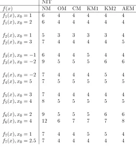
All done computations by MATHEMATICA software has 120 digit oating point arith-metic (Digits:=120). An approximate solution quite is accepted as exact root, depending on the precision () of the computer. Criterias jxn+1 xnj < and jf(xn+1)j < are used

for computer programs, and so, when the stopping criterion is satised, xn+1 is taken as

the exact root . For numerical illustrations, the xed stopping criterion = 10 15_{, is}

used.

In comparison the Newton's method (NM) with the well-known fourth-order Os-trowski's method [5], (OM), dened by

xn+1 = xn (1 +_f(x f(yn) n) 2f(yn))

f(xn)

f0_(xn); (3.27)

yn= xn _ff(x_0(xn)

n); (3.28)

and (CM), [2], dened by

xn+1= yn [_f(xf(xn) n) f(yn)]

2 f(yn)

f0_(xn); (3.29)

yn= xn _ff(x_0(xn)

n); (3.30)

the other method, (KM1), [4],

xn+1= xn (1 + R(xn) + 2R2(xn) + 5R3(xn) + )_ff(x_0(xn)

n); (3.31)

R(xn) = _f(xf(yn)

n); (3.32)

yn= xn _ff(x_0(xn)

n); (3.33)

the Kou et al.'s method [3], (KM2),

xn+1= xn f

2_{(xn) + f}2_(yn)

yn= xn _ff(x_0(xn)

n); (3.35)

and (AEM) dened by (2.10)-(2.12), in the present contribution, the same examples in Changbum Chun [1] are used.

f1(x) = x3+ 4x2 10, f2(x) = x2 ex 3x + 2, f3(x) = xex2 sin2(x) + 3 cos (x) + 5,

f4(x) = sin (x)ex + ln (x2+ 1), f5(x) = (x 1)3 2, f6(x) = (x + 2)ex 1, f7(x) =

sin2_{(x) x}2_{+ 1.}

Table 1: Comparison of the number of iterations (NIT ) in (NM), (OM), (CM), (KM1), (KM2) and (AEM) methods

NIT

f(x) NM OM CM KM1 KM2 AEM

f1(x); x0= 1 6 4 4 4 4 4

f1(x); x0= 2 6 4 4 4 4 4

f2(x); x0= 1 5 3 3 3 3 4

f2(x); x0= 3 7 4 4 4 4 5

f3(x); x0= 1 6 4 4 5 4 4

f3(x); x0= 2 9 5 5 5 6 6

f4(x); x0= 2 7 4 4 4 5 4

f4(x); x0= 5 7 5 5 5 5 5

f5(x); x0= 3 7 4 4 4 4 4

f5(x); x0= 4 8 5 5 5 5 5

f6(x); x0= 2 9 5 5 5 6 6

f6(x); x0= 4 12 6 7 7 7 8

f7(x); x0= 1 7 4 4 5 5 4

f7(x); x0= 2:5 7 4 4 4 4 4

4 Conclusion

In this paper, a family of new iterative methods were dened and analyzed for solving non-linear equations and also it was proved that the order of convergence of these methods is at least four.

References

[1] C. Chun, Y. M. Ham, Some sixth-order variants of Ostrowski root-nding methods, Applied Mathematics and Computation, 193 (2007) 389-394.

[3] J. Kou, Y. Li, X. Wang, A composite fourth-order iterative method for solving non-linear equations, Appl. math. comput. 184 (2007) 471-475.

[4] J. Kou, Second-derivative-free variants of Cauchy's method, Applied Mathematics and Computation, 190 (2007) 339-344.

[5] A. M. Ostrowski, Solutions of Equations and System of Equations, Academic press, New York, 1960.