Velocity tracking of cruise control system by using feedback linearization method

(1)

*

Esmaeel Khanmirza

Email Address: khanmirza@iust.ac.ir 10.22068/ijae.8.4.2826

Velocity tracking of cruise control system by using feedback linearization method

Ehsan Alimohammadi1, Esmaeel Khanmirza1*, Hamed Darvish1

1

School of Mechanics, Iran University of Science and Technology, Narmak, Tehran, Iran

ARTICLE INFO A B S T R A C T

Article history:

Received: 28 Apr 2018 Accepted: 29 Nov 2018 Published: 01 Dec 2018

In cruise control systems, the performance of the controller is important. Hence, in order to have accurate results, the nonlinear behavior of a vehicle model should also be considered. In this article, a vehicle with a nonlinear model is controlled by using a nonlinear method. The nonlinear term of the model is the generated torque of engine, which is a polynomial equation. In addition, feedback linearization is used as a nonlinear method in order to design two parallel controllers to control the movement of the vehicle. These two parallel controllers are used to control braking and gas pedals which are in charge of the angular velocity of the wheels. To check the performances of controllers, first, each controller is used separately. Finally, two parallel controllers are used to track the reference signal. Comparison between results shows that the designed controller is able to reduce the convergence time of about 10 seconds. This improvement is near 35% in comparison with near studies. In addition, it can reduce the error between the velocity of the vehicle and the values of the reference signal that results in more safety for passengers.

Keywords:

cruise control nonlinear model generated torque

feedback linearization parallel controllers

International Journal of Automotive Engineering

Journal Homepage: ijae.iust.ac.ir

S

N:

2

0

8

-9

8

9

(2)

International Journal of Automotive Engineering (IJAE) 2827

1 Introduction

Nowadays the world population is growing fast and roads do not have enough space for vehicles. Increasing number of vehicles and human error can cause accidents and as a result, traffic congestion occurs. It is estimated that human error causes a majority of accidents [1]. There are some solutions for handling this problem. Improving the quality of the roads is a solution that is not efficient due to environmental concerns. Intelligent Vehicle Highway Systems (IVHS) is another solution. Advanced Traffic Management Systems (ATMS), Advanced Vehicle Control Systems (AVCS) and Advanced Public Transportation Systems (APTS) are some major components of IVHS. The exciting aspect of IVHS is a new concept in using information technology to solve transportation problems [2].

In recent years, vehicle manufacturers have used intelligent control systems in their products, because they bring comfort. Some intelligent control systems are “advanced driver assistance systems” (ADAS) such as “adaptive cruise control” (ACC) and collision avoidance system. Using control approaches can facilitate the traffic flows and improve the performance of the traffic system [3]. One of these control approaches is “cruise control” (CC) that has been popular in recent years [4]. CC system can be assumed as a safety system in vehicles. The main task of this system is to keep a safe distance between vehicles [5]. One of the ways of this approach is to obtain the velocity that the driver chooses on the road. There are some other systems that have been used in researches. Nowadays for instance “Stop and go cruise control systems” and ACC systems are used in vehicles. ACC systems can act with the velocity more than 40 km/h, and stop and go systems work in low velocities [6].

ACC and stop and go systems have a problem, which is controlling the amount of speed [7]. ACC system at first did not have any mechanism to control and it worked just by opening and closing the engine valve, which was not efficient in urban driving [8]. In [9], a user-friendly expert system was designed to signalization for isolated intersections. In

[10], a genetic-fuzzy ABS controller was designed that reduced the vehicle stopping distance. In [11], in order to prevent the

accident, a fuzzy controller was used that imitated human logic to convert them into fuzzy rules. The fuzzy controller consists of fuzzifier, inference engine, and defuzzifier. First, by using membership functions, real values will be converted to fuzzy values. These values are between zero and one. By using fuzzy values, the inference part creates output values and defuzzifier converts them to real output values. In [12], a fuzzy controller was used to reduce disturbance of transition between CC and ACC. Recent studies have shown that neural network has been used, too. In [13], the neural network was used in different situations to produce acceleration and deceleration forces. ”Back propagation network” (BPN), “radial basis network” (RBN), and “generalized regression neural network” (GRNN). Results showed that BPN satisfies safety constraints better and RBN satisfies comfort constraints better. In [4], authors improved reference signal and then by using ’proportional integral derivative’ (PID) controller, they prevented the collision between two vehicles.

In many kinds of research like [14, 15] without considering initial conditions, the controller has been designed that can track acceleration and deceleration. These researches showed that when the controller starts, the difference between the initial condition and the reference signal is low, and an increase in this difference will result in the collision.

In CC systems after choosing the desired velocity by the driver, they can work without needing anymore action by the driver. Hence, it helps the driver to rest in long distance. In recent studies, researchers have used a linear model of vehicle or linearized equations of its movement to design controller.

In this article, we have used a nonlinear longitudinal equation of motion for a vehicle. The nonlinear term is the generated torque and we have used feedback linearization, a nonlinear method, to control it. First, we began with a 2D model of a vehicle with engine and braking torque and ground reaction torque of wheels. Then we have designed a controller for each gas and braking pedals. Finally, we have combined these two controllers to control the vehicle movement.

2 Vehicle model

To simulate the dynamical behavior of a vehicle, we should consider it as a single and

(3)

2828 International Journal of Automotive Engineering (IJAE) big body and then we can test motion

dynamical behavior. Analyzing of this dynamical behavior is possible by considering the vehicle as a wheel, two wheels or four wheels [16, 17]. In cruise control, usually, the longitudinal dynamic is required for analysis. Hence, in figure (1), 2D view of the vehicle is shown.

In figure (1), m is the mass of the vehicle and V is the velocity in the X direction. Index r and f show front and rear wheels that have angular velocity ω. J is the moment of inertia and µ is the friction coefficient between wheels and ground. B, C, L, and H are the distances between the center of gravity and front and rear wheels or ground. The inputs of this model are gas and braking pedals and output is angular velocity and as a result, longitudinal velocity will be obtained [18].

Figure 1.2D view of the vehicle

In the vehicle, first by pushing the gas pedal, fuel enters the engine. The engine generates the torque which is proportional with the gas pedal and this torque will be applied to the wheels [19]. In addition, the braking signal generates torque, which is needed for the vehicle to stop. By considering the vehicle as a single mass, acceleration from generated torque will be calculated. Eq. (1) shows the angular acceleration of the vehicle wheels. This equation is equal for each wheel.

̇ (1)

In Eq. (1), is the generated torque of the engine, is the generated torque of braking and is the generated torque of friction adherence. By considering a constant coefficient known as the coefficient of torque of friction adherence , will be obtained by Eq. (2).

By using these equations, we can calculate the longitudinal velocity of the vehicle. We should multiply ω by wheel radius r.

(2)

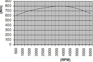
The generated torque of the vehicle includes some sections such as torque converter, gearbox, and differential that generates needed force for wheels. To analyze this torque of the engine, we consider Benz V8, which its capacity is 800 Nm with rotation 3700 rpm of the motor. Figure (2) displays the generated torque of the engine. To simulate generated torque, an equation that represents the relation between engine rotation and torque is required. This equation will be obtained by using amounts of the figure (2) and a polynomial.

(3)

Figure 2.Relation between engine rotation and

generated torque in Benz V8

Consider that is gear coefficient, and is a differential coefficient. Therefore, engine rotation R will be:

(4) By considering past equations and delays for transferring torque to wheels, the transfer function between gas signal and wheel torque reads [20]:

(5)

Where is gas signal that is between zero and one.

In the simulation of the braking system, there is a braking signal that generates required pressure with some delay to activate braking discs. So the relation between braking pressure and braking signal could be as follows [20].

(6)

Where is the braking signal that is between zero and one.

After achieving the required pressure, generated torque of braking can be written as:

(4)

(7)

In equation (7), K is converter coefficient in braking. When the velocity is much less than α, it remains as zero, in order that the system does not decelerate.

3 Feedback linearization

Feedback linearization is a controller design method that has been used in recent years. In this method, after using exact transformations of state and feedback, we use an input to delete nonlinear terms of the model and to linearize the system. This method is different from the linearization method because we do not use the approximation of equations. After using this method, we can design a linear controller to control the system. Feedback linearization has some problems. For example, it requires exact information of the system [19].

In this article, first, we consider that the system is in the acceleration mode. Hence, the driver should push the gas pedal and the vehicle will accelerate. In this mode, = 0 and equation (1) will be converted to equation (8) and the input is just or gas pedal.

̇ (8)

Final equation will be:

̇

(9)

We consider y = ω, and according to the equation (9), in the first derivative ( ̇ ̇ ), the input variable appears. Hence, feedback linearization is implementable. Now, we need an input variable to delete nonlinear terms of equation (9), so we will have a linearized equation in order to design controller.

According to the equation (9), is defined as:

(10)

So, the equation of the equivalent system will be:

̇ (11)

Where v is:

̇ (12)

Equation (12) should be stable and it depends on amounts of k1. By using Roth-Hurwitz stability criteria we know that k1 should be greater than zero. is an error function and its equation is:

(13)

Where is the desired output of the system. Finally, the equation of reads:

(14)

When the system is in the deceleration mode, or in another word when the driver wants to reduce speed, he should push braking pedal and the vehicle will decelerate. In this mode, = 0 and equation (1) will be converted to equation (15) and the input is just or braking pedal.

̇ (15)

Now, we act like acceleration mode, so the new equation of ω˙ will be:

̇

( ) (16)

Finally, according to the equation (9), is defined as:

( ₎

₍₁₇₎

Where v is equal to equation (12) with a constant coefficient . Hence, the final equation of is:

( ₎

(18)

Note that in equations (14, 18) is the desired angular velocity. To achieve desired longitudinal velocity we should use two parallel gas and braking mode controllers together.

Required parameters are brought in table (1).

4 Results of the gas pedal controller

In this section, we consider gas pedal controller and check its performance in increasing velocity. Suppose that the velocity of the vehicle is 5(m/s) and we want to achieve the velocity of 15(m/s).

Figure (3) shows the controller performance in achieving the desired velocity.

(5)

2830 International Journal of Automotive Engineering (IJAE)

Table 1. Parameters

Parameter Value

L 3 m

B 1.5 m

C 1.5 m

0.1 Nm/rads−1

0.2 s

2.82

3.56

α 0.0001

13.33 Nm/bar

6.66 Nm/bar

M 1626 kg

J 4.5 kg/m2

r 0.3 m

k1 20

k2 300000

Figure 3.Performance of gas pedal controller

5 Braking pedal controller

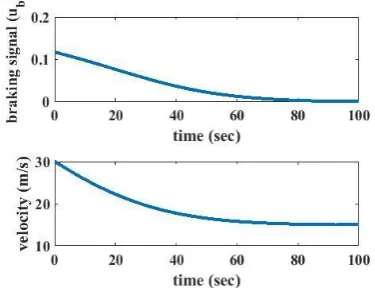
To check the performance of braking pedal controller we consider that the velocity of the vehicle is 30(m/s) and we want to reduce it. So figure (4) shows that this controller acts properly.

Figure 4.Performance of braking pedal controller

6 Tracking reference signal by using two

parallel controllers

We should consider the initialization states of the system in designing the system controller. Suppose that the value of the reference signal is greater than the velocity of the front vehicle and the real velocity of the vehicle is between those two. Because the velocity of the vehicle is smaller than the value of the reference signal, the vehicle should increase velocity so that the value of reference signal be decreased to avoid the collision between vehicles. This increasing velocity of the main vehicle causes the collision between vehicles. To solve this problem, the difference of real velocity of the vehicles should be added to the equation of the reference signal. If the difference is large, it will decrease the magnitude of the reference signal. Eq. (19) shows the reference signal that is used in this article and has improved.

( ) (19)

In equation (19), a and are 0.005 and 0.5 respectively, is the cruise control velocity, and and are the velocity of the front and main vehicle. In this section, we use two parallel controllers, which control gas and braking pedals to track reference signal. Figure (5) shows tracking the reference signal. Figure (5a) is from [4] and figure (5b) is the result of this article. As it is shown, in this article we have used the more accurate model of the vehicle which had nonlinearity terms and we have improved the tracking time near 10s or 35%. Also, the difference between amounts of the reference signal and tracking signal in figure (5b) is less than figure (5a). Hence, we have improved the performance of the controllers by using a nonlinear method to design the controller.

(6)

Figure 5.Comparison between two tracking reference

signal. Figure (5a) is from [4] and figure (5b) is the result of this article

7 Conclusion

In this article, we have used a nonlinear longitudinal model of the vehicle which is more accurate than recent studies, due to considering nonlinear terms. Also, we have used a nonlinear method which is feedback linearization, to design the controller in order to control longitudinal motion of the vehicle. At first, we have used two separate controllers which control braking and gas pedals to check their performance. Afterward, we have combined these controllers to track a reference signal in order to avoid collision between this vehicle and the front one. As it is shown in figure (5), reaching the convergence is faster in comparison with [4], from 30 to 20 seconds which is about 35%. Also, as it is shown, the difference between the amount of tracking signal and reference signal is less which shows improvement of controllers’ performance in comparison with [4].

References

[1] Peters, G. A. and Peters, B. J., “Automotive

vehicle safety”, CRC Press, (2003).

[2] Faghri, A., S., Panchanathan and R. S.,

Nanda, “Intelligent vehicle highway systems (IVHS) issues and recommendations”, Journal of

Engineering, Islamic REpublic of Iran,

(1995), 121– 131.

[3] Baskar, L. D., Schutter, B., Hellendoorn, J.

and Papp, Z., “Traffic control and intelligent vehicle highway systems: a survey”, IET Intelligent Transport Systems, (2011), 38–52.

[4] Mohtavipour, S. M., Darvish Gohari, H. D.

and Shahhoseini, H. S., “Improvement of adaptive cruise control performance by considering initialization states”. Universal

Journal of Control and Automation, (2015),

53–61.

[5] Kyriakopoulos, K. J. and Skounakis, N.,

“Moving obstacle detection for a skid-steered vehicle endowed with a single 2-d laser scanner”, In Robotics and Automation, 2003. Proceedings. ICRA’03.

IEEE International Conference on, Vol. 1,

(2003), 7–12.

[6] Sanchez, F., Seguer, M., Freixa, A.,

Andreas, P., Sochaski, K. and Holze, R., “From adaptive´ cruise control to active safety systems”, Technical report, SAE

Technical Paper, (2001).

[7] Iijima, T., Higashimata, A., Tange, S.,

Mizoguchi, K., Kamiyama, H., Iwasaki, K. and Egawa, K., “Development of an adaptive cruise control system with brake actuation”, Technical report, SAE Technical

Paper, No. 2000-01-1353, (2000).

[8] Naranjo, J. E., Gonzalez, C., Garc´ ´ıa, R.

and De Pedro, T. “Acc+ stop&go maneuvers with throttle and brake fuzzy control”, IEEE Transactions on intelligent

transportation systems, (2006), 213–225.

[9] Faghri, A., ”Signal design at isolated

intersections using expert systems technology” Journal of Engineering,

Islamic Republic of Iran, Vol. 8, No. 4,

(1995), 181–189.

[10] Mirzaei, A., Moallem, M. and Mirzaeian,

B., ”Designing a genetic-fuzzy anti-lock brake system controller”, International

Journal of Engineering, Vol. 18, No. 2,

(2005), 197–206.

[11] Batayneh, W., Al-Araidah, O., Bataineh, K.

and Al-Ghasem, A., “Fuzzy-based adaptive cruise controller with collision avoidance and warning system”, Mechanical

Engineering Research, (2013).

[12] Sathiyan, S. P., Kumar, S. S. and

Selvakumar, A. I., ”Optimised fuzzy controller for improved comfort level during transitions in cruise and adaptive cruise control vehicles”, In Signal

Processing And Communication

Engineering Systems (SPACES), 2015

International Conference on, (2015), 86–

91.

[13] Cherian, M. and Sathiyan, S. P. “Neural

network based acc for optimized safety and comfort”, Int J Comp Appl, (2012).

[14] Ganji, B., Kouzani, A. Z., Khoo, S. Y. and

Shams-Zahraei, M., ”Adaptive cruise control of a hev using sliding mode control” ,Expert systems with applications, No. 2, (2014), 607–615.

[15] Milanes, V., Villagr´ a, J., Godoy, J. and

Gonz´ alez, C., “Comparing fuzzy and intelligent pi´ controllers in stop-and-go manoeuvres”, IEEE Transactions on

(7)

2832 International Journal of Automotive Engineering (IJAE)

Control Systems Technology, No. 3, (2012),

770–778.

[16] Martinez, J. J. and Canudas-de Wit, C.,

“Model reference control approach for safe longitudinal control”, In American Control

Conference, 2004. Proceedings of the 2004,

Vol. 3, (2004), 2757–2762.

[17] Zoroofi, S., ”Modelling and simulation of

vehicular power systems”, Chalmers

University of Technology, (2008).

[18] Rajamani, R. “Vehicle dynamics and

control”, Springer Science & Business

Media, (2011).

[19] Shakouri, P., Ordys, A. and Askari, M.

R., ”Adaptive cruise control with stop&go function using the state-dependent nonlinear model predictive control approach”, ISA transactions, No. 5, (2012), 622–631.

[20] Short, M., Pont, M. J. and Huang, Q.

“Simulation of vehicle longitudinal dynamics”, Safety and Reliability of

Distributed Embedded Systems, (2004),

01–04.