Second Order Sliding Mode Observer-Based Control for Uncertain Nonlinear MEMS Optical Switch

Se

C

The main adv of an optical s scale matrix networks no conversion conversion. T slow bit rates optical switch Optical switc in telecomm network (AO electronics.

1. Assistant Pr 2. PhD Studen

cond

Contr

Introd

vantageof an o signal to anoth switches whi ow are rea or electronic These switches s capacity. To c h has been pro ches became im munications ind

ON), which m

rofessor (Corres nt

Orde

rol for

artment of M

This paper studi rical, mechanic ficant merits i ever, an inhere h position infor avated by consi rvers based on ate the state v rvers are then rmances. The ering phenome hermore, since

rbances/uncerta control is pr ating any swit ol have good tr

words: Robustnes optical sw

duction

optical switch i her signalin a d ichare mostly alized by o c switching/e s are very exp circumvent the oposed as an o mportant becau dustryto focus means thetota sponding Autho

er Slid

r Unc

Opt

H. F

rmation at all t idering disturba

the first order variables of the utilized in the newly invented ena as the ma

e second or ainties which v roposed to enh tching time. Si racking ability a

s, second order s witch

is the conversio direct way. Lar

used in optic optical-electron electronic-optic ensive and ha ese problems,t obvious solutio

use of the desi s on all-optic al exclusion

or)

ding M

ertain

tical S

Fazeli

and F

ngineering, M rospace Rese

*_{Tehran, IR}

midfaz2000@

n nonlinear dyn al subsystems.

control voltag n designing co times due to th ances. In order and second or e device subjec

control system d second order in drawback o rder sliding vary with states hance the robu imulation resu and robustness

sliding mode obse

on rge cal nic cal ave the on. ire cal of use o perfo mani them very produ weig integ nume preci instan ofcon for t advan techn reliab

Mode O

n Non

Switch

F. Rahimi

MalekAshtar earch Institut

RAN @yahoo.com

amics of a MEM Recently, MEM ge requirement ontrol for such

e saturated out r to circumvent rder sliding mod

ct to external m to maintain r

r sliding mode of the first ord mode contro s, a new time-v ust performanc ults show that against disturb

erver, second ord

One approach of MEMS tech orm the switc ipulate optical m to electronic attractive be uctioncost, c ght, fast bit gration, and o

erous applicat ision in posit nce, in medic ncentrating on the purpose o nced space nologies to d

bility, while

Obser

nlinear

h

2

r University o te

MS optical swit EMS optical sw ts and power systems is un tput characteri t this problem, de approach ar

disturbances. T robust stability e controller ca der sliding mo l is not ro varying second ce of the contr

the proposed bances

_.

der sliding mode

h to optical s hnology to fab ching functio l signals direc

signals. MEM ecause of the compactness,

rates, low optical transp tions for optic tioning of th cal science the

n the particul of detection a missions dramatically e

e reducing

rver-B

r MEM

of Technolog

tch addressing witch has had

consumption. availability of istics, which is two nonlinear re designed to The nonlinear y and tracking an remove the ode controller. obust against d order sliding

roller without observer and

control, MEMS

switching has bricate tiny m on. These tin ctly without c MS optical sw eir high capa small size power con parency[1, 2]. cal switches th he micro-actua

ese devices ar lar medical p and therapy. are offeri enhance the s the cost o

Based

MS

gy

50

/

transportation. Generally, it costs 25,000 US$ to put one kilogram of a payload in the Earth orbit. Therefore, MEMS devices are essential for the future space missions. The analog nature of MEMS actuators and their device characteristic uncertainties, due to the manufacturing tolerances, make the implementation of device impractical and/or require costly calibrations. In addition, the nonlinear characteristics of MEMS actuators could result in instability over an extended actuation range in the open-loop operation. This added complexity combined with the submicron precision requirement calls for the development of comprehensive dynamic modeling frameworks along with robust controllers.

Several control strategies have been proposed in the literature for the MEMS optical switch. Owusuet al. [3] designed a controller based on the feedback linearization to compensate the nonlinearity in the system dynamics, and succeeded in stabilizing theswitch position of the MEMS optical switch. However, the result was not acceptable by applying the disturbances/uncertainties to the plant. Ebrahimietal.[4] presented a robust controller based on the traditional sliding mode theory for a MEMS optical switch. Vali et al. [5] introduced the quantitative robust feedback theory to control a nonlinear MEMS optical switch in the presence of parameter variations and unknown disturbances. One of the most important differences between “macro-scale” and “micro-scale” control design is the added modeling uncertainties and nonlinearities in“micro-scale”. Hence, the implementation of the proposed controller is attenuated by increasing the inherent complexity of the system.

For the stabilization of anoptical switch, it is necessary to dynamically estimate the switch position and velocity. Because, when the switch is near the completely closed or open situation, there is no position information available as a feedback for the control system. Thus, state observers have been introduced to overcome this problem. In [3] a simple nonlinear observer is used to estimate the state variables for a system with Lipschitz nonlinearity in the output characteristics. In this paper, two sliding mode observers are proposed to estimate the state variables for an uncertain nonlinear system. The main advantages of the sliding mode observer are robustness against disturbances/unmodeled dynamics, insensitivity to parameter variations, compact implementation and efficiency for the standard output system.

This paper consists of three major parts. In the first part, two robust sliding mode observers are considered to estimate the switch position and velocity of a MEMS optical switch in the presence of an unknown, but bounded disturbance: 1) first order sliding mode observer (FOSMO) based on the Lyapunov second method [6,7] and 2) second order

sliding mode observer (SOSMO) based on the super-twisting algorithm (STA) [8]. In practice, the second order sliding mode observers are used to estimate the velocity of the system independent of the controller design and they are still successfully implemented to solve the various problems.

In the second part, the estimated state variables are utilized to design the sliding mode controllers. Theyenable the compact realization of a robust controller, tolerant of device characteristics variations, nonlinearities, and types of inherent instabilities. The main drawback of this approach is the high frequency switching called chattering, which can excite the unmodeled high frequency dynamics and make the system unstable [9]. Second order sliding mode control based on STA is one of the recently developed techniques to overcome this difficulty. Here, the discontinuous control acts on the second derivative of the sliding variable instead of the first derivative in the traditional sliding mode control to remove the chattering effect while preserving the advantages of the traditional sliding mode control [10, 11]. Despite the popularity of the STA, it has a major flaw. STA is not robust against disturbances/uncertainties that change with the state variables. One of the methods to enhance the robust performance in the SMC theory is to eliminate the reaching phase using the time-varying sliding mode control (TVSMC) strategy. The concept of TVSMC was introduced by Choi et al. [12] and Bartoszewicz [13]. TVSMC can shorten the reaching phase via a shifting or rotating sliding surface. Yongqianget al. [14] studied the attitude stabilization of a rigid spacecraft based upon the different TVSMCs by designing the switching time between sliding surfaces. In the previous papers, the designed sliding surface included switching time and the designed controller pertained against the initial conditions to shift or rotate the sliding surface. In the present paper, we propose a new TVSMC algorithm without describing the switching time and a designer is able to select both time-varying function and a procedure to shift (known as “intercept-varying”) and/or rotate (known as “slope-varying”) the sliding surface optionally for every initial conditions. As a result, the main contributions of this paper are to employ:

Robust observers and controllers simultaneously based on the first- and second-order sliding mode control theories for the MEMS optical switch. These devices can be used in space missions (e.g. remote sensing and communication satellites) because of the presence of high resolution and reliability, and minimum weight, size and power consumption.

Mathematical Model

A general optical switch structure consisting of an electrostatic comb drive, the body of the device, and a blade or shuttle is shown in Fig.1. Thevoltage applied to the comb drive actuator generates a force that moves the shuttle attached micro-mirror that cuts a light beam exiting a transmitting fiber and being collected in a receiving and modulating density.

In order to derive a mathematical model of system dynamics it is needed to determine parameters of the relevant differential equation that describes forces acting on the shuttle. It is assumed that the shuttle has one degree of freedom and moves only in one direction. It is important to mention that there might be other degrees of freedom, like rotation around the main body axes, translation along them, as well as different vibrational modes. However, only the main degree of freedom will be considered in this paper and also the related materials for modeling purpose are referred to [15].

The mathematical model of the switch has three main components: an electrical, a mechanical and an optical component. Altogether, the system can be described with a second order nonlinear differential equation as:

+ ( , ) + ( ) = ( , )

= ℎ( )(1) (1)

wherem is the effective moving mass of the shuttle, d is a function describing losses such as damping and friction, k is the stiffness of the suspension, f is the electrostatic force acting on the model, P is light intensity and x is the shuttle position.

Figure 1. Image of a MEMS optical switch

The system exact parameters m, d, k and f are not easy to obtain and we will go step by step to determine all of these parameters. First, the electrical model is built and thenthe optical model connects the position of the shuttle to the intensity of the sensed light.

Electrical Model

The electrical part of the model considers generation of the induced electrostatic force by applying voltage to the actuator. The capacitance of the comb drive as a function of position should be determined first. Capacitance of the comb drive can be calculated as the sum of all of parallel capacitances among pairs of comb electrodes. The total capacitance is given as a function of position by[15]:

( ) =

= ( ) (2)

where = 8.854 × 10 is the dielectric constant of vacuum, n is the number of the movable comb fingers (n=150), T is thickness of the structural layer ( = 35 ), is the length of the gap between fingers ( = 2.6 ) and is the overlapped length of fingers when no voltage is applied ( = 15 ). At rest position, the capacitance of the comb drive is about 0.27 when = 0 and = 15 , which increases as force is applied and the fingers move closer. Generally, the electrostatic force of the capacitor is given as theproduct of squared voltage and change of capacitance with respect to position as:

( , ) = (3)

whereVis the voltage applied over the electrodes. By combining (2) and (3) electrostatic force can be calculated as:

( , ) =

=

(4)

where is defined as the input gain ofthe system with the value of = 17.8 ⁄ .

It is interesting to note that capacitance (2) depends linearly on position over a wide range of deflections. It is one of the most important characteristics of the comb drive. Generally, for other configurations, this is not the case and capacitance is a higher nonlinear function of position . It should be noted that the linear relationship does not hold for extreme deflections and may cause considerable undesired results that necessitate using a robust control scheme to meet such uncertainties.

Mechanical Model

In order to obtain the mechanical model of the system, three parameters namely, the effective moving mass m, the damping coefficient d and stiffness of the suspension khave to be determined.Effective mass for the switch can be expressed as [15]

= + + 2.74 (5)

52

/

Stiffness is generally a nonlinear function of position f=k(x). For most metals and for silicon spring-like structures, it can be described as ( ) = +

. For the suspension given in this paper, stiffness of the beam is assumed to be a linear function of the position and its coefficient is given as = = 0.46 ⁄ .

Damping, or energy dissipation, is the most difficult parameter to be determined analytically, despite usingFEA. The reason lies in the number of different mechanisms that cause it including friction, viscous forces, drag, etc. We will consider viscous forces as theprimarycauses of damping. Four different mechanisms contribute to damping, Couette flow, Poiseuille flow, Stokes flow, and Squeeze film damping [16]. Generally, they can be summarized as

= ( + ) . When actual parameters are

substituted, damping is expressed as [17]:

( , ) = 0.0363( + 15 × 10 ) (6)

Optical Model

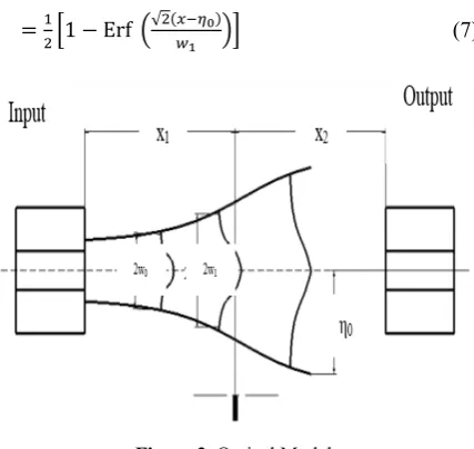
The optical model is simply a function that connects the intensity of light to the position of the blade as in Fig.2. Light beam is intercepted by the blade, increasing and decreasing the throughput of light. The Rayleigh-Somerfield model is based on a Gaussian distribution of the intensity across the light beam.

Transmitted power can be described as [17]:

= 1 − Erf √ ( ) (7)

Figure 2. Optical Model

where = 10.9 and = 11.2 .

The relationship between the power ratio and the position of the mirror is shown in Fig.3.It is important to note that the attenuation curve is saturated by the error function which makes it difficult to reconstruct the states in saturation region for control design purposes.

Figure 3. Power ratio against displacement

Consequently, integrating the created models for each section and applying the procedures done for increasing accuracy of the model in [2], result in the nonlinear mathematical model of the switch as:

=

. × [−(0.0363 + 4.5 ×

10 ) − 0.6 + 1.9 × 10 + ( , , , )]

(8)

where (quadric term in voltage) is the input and represents the uncertainties affecting the MEMS optical switch which is assumed to be bounded toa positive known term ( , , ). As mentioned above, these uncertainties mostly come from simplifications in electrical and mechanical model of device.

Design of Sliding Mode Observers

Sliding mode observers are very useful means which have been developed for many reasons like working with reduced observation error dynamics, possibility of obtaining a step by step design, a finite time convergence for all the observable states and robustness against uncertainties [6].

At first, a traditional first order sliding mode observer (FOSMO) is proposed. The well-known problems whenusing the FOSMOs are the relative degree one requirement and the chattering phenomena. In order to deal with these limitations while preserving the main advantages of the FOSMOs such as finite-time convergence and robustness against disturbances, second order sliding mode observers (SOSMO) are proposed for system state observation. This kind of observer does not require the relative degreeof the sliding manifold to be one, and can totally remove the chattering effect [8].

0 0.5 1 1.5 2 2.5

x 10-5 0

0.1 0.2 0.3 0.4 0.5 0.6 0.7 0.8 0.9 1

Displacement(m)

P

owe

r Ra

First Order Sliding Mode Observer (FOSMO) Design

The state space representation of (8) can be rewritten as:

=

= − − ( + )

+ + ( , , , )

=

(9)

where = [ ] , and , denote the switch position and velocity, respectively.

Lets consider a traditional sliding mode observer for the MEMS optical switch (9) as [6]:

= + sign( − )

= −

−1( + ) + sign( − )

+ + sign( sign( − ))

(10)

By taking = − , the error observation dynamics are obtained from (9) and (10) as:

= − sign( )

= −1( + ) − sign( )

+ ( , , , ) − sign( sign( ))

(11)

Now, let us consider the nonempty manifold = = 0in which the attractivity of is proved by using the second method of Lyapunov. Let the Lyapunov function be = . Differentiating with respect to time results in:

=

= − sign( )

(12)

Obviously, if is chosen sothat > | | , then

< 0 is sufficiently ensured. It means that by decreasing the Lyapunov function with respect to time, the convergence to the sliding surface = 0 will be obtained in finite time . In other words, for > | | , converges to in finite time and remains equal to for > . Moreover, for > , _≈0, so that from (11)

= sign( ) (13)

After time , the observantion error dynamics are now equal to

= 0

= ( , , , ) − sign( ) (14)

By setting = ( + ),

= +

= ( , , , ) − sign( ) (15)

Consequently, goes to zero in finite time >

if > ( , , ). In practice, the signum function

sign( ) can be replaced by a continuous function _{| |} to alleviate chattering, where is a positive scalar constant.

Second Order Sliding Mode Observer

(SOSMO) Design

In order to estimate the state variables of the MEMS optical switch without chattering effect, the following second order sliding mode observer is designed as [8]

= + | − | ⁄ _{sign( − )}

= − −1( + )

+ + sign( − )

(16)

where represents the observed state and , are the second order sliding mode observer gains.It is important to note that the initial moment (0) =

(0) and (0) = 0are taken to ensure the observer convergence.

By taking = − , the error observation dynamics are obtained from (9) and (16) as:

= − | | ⁄ _{sign( )}

= −1( + ) + ( , , , )

− sign( )

(17)

In our case, the system states are bounded, then the existence is ensured of a constant , sothat the inequality

( , , , ) −1( + ) < (18)

holds for any possible , , and | | ≤

2 . and are defined sothat ∀ ∈

ℝ , ∃ , : | | ≤ , | | ≤ . The state boundedness is true, sincethe control input V isbounded(0 < < 35 ) based on the system

hardware [18]. Consequently, the system (8) is bounded input bounded state stable, because for each initial state and each bounded input, the corresponding solution is bounded for > 0. Therefore, can be written as:

= ( + ) + (19)

Let and satisfy the following inequalities:

>

54

/

where ́ is some chosen constant, 0 < ́ < 1.

Theorem1: Suppose that the parameters of the

observer (16) are selected according to (20), and condition (18) holds for system (9). Then, the variables of the proposed second order sliding mode observer (16) converge in finite time to the state variables of system (9), i.e., ( , ) → ( , ).

Proof. The proof was given by Davila and Fridman in

[8].

Sliding Mode Control Design

In this section, the sliding mode theory is employed to control the switch position of a MEMS optical switch. By ensuing that the sliding mode observation is obtained in the previous section, a particular type of variable structure controller (VSC) scheme is presented to combine the controller and observer.

At first, a traditional first order sliding mode controller (FOSMC) is proposed for the nonlinear uncertain system. Based on the traditional sliding mode theory, the system state satisfies the dynamic equation that governs the sliding mode all the time. This requires infinite switching that causes chattering as a main drawback of this approach as it may excite unmodeled high frequency dynamics of the system[9]. The second order sliding mode control (SOSMC) scheme is one of the recently developed techniques which can overcome this difficulty. Here, the discontinuous control acts on the 2nd_{derivative of sliding variable instead of the}

first derivative in the traditional sliding mode. This group of controllers does not require the relative degree to the sliding manifold to be one, and can totally remove chattering effect and preserve the main advantages of the traditional sliding mode such as finite time convergence and robustness against uncertainties.

In each part of the control design processes, i.e. FOSMC and SOSMC, at first, we assume that the actual switch position and velocity are available. It helps to investigate the effects of using the observed state variables, rather than actual state variables, on the characteristic response of the closed-loop system. Then, two different controls are presented by using the estimated state variables which are obtained by the designed nonlinear observers in the previous section due to the unavailability of the state variables for measurement in practice.

First Order Sliding Mode Control (FOSMC) Design

In the first case, to design the robust sliding mode control, the sliding surface ( = 0)is considered using actual states from (9) with observability assumption of the system. This expression can be written in the form of

= − + ( − )

= 0

(21)

To ensure that the actual states of the system approach the sliding mode, = 0should be satisfied. Substitution of the actual states from (9), results in the following expression for equivalent control, .

= { + ( + ) + [ −

( − )]} (22)

Finally, the sliding mode control law (input voltage) with availability of the system states assumption will be as:

= − sign( ) (23)

where is a constant parameter depending on the disturbance exerted on the system and reaching time. By using the second method of Lyapunov, let the Lyapunov function be = . Differentiating with respect to time results in

=

= − sign( ) + ( )

≤ (− sign( ) + )

(24)

Obviously, if ≥ is satisfied, then < 0 is sufficiently ensured.

In the second case, to design sliding mode observer-controller, the sliding surface ( ̂ = 0) is considered using the estimated states from traditional FOSMO dynamics (10) and/or SOSMO dynamics(16). This expression can be written in the form of

̂ = − + ( − )

= 0

(25)

Also, to ensure that the estimated states of the system approach the sliding mode, ̂ = 0should be satisfied. Substitution of the estimated states from traditional FOSMO (10), results in the following expression for equivalent control, .

= { + ( + ) +

sign( − )

− sign sign( − )

+ [ − ( + sign( − ) − )]}

(26)

On the other hand, substitution of the estimated states from SOSMO (16), results in the following expression for equivalent control, .

= 1 { + ( + )

+ − + | − | ⁄ _{sign( − )}

− ) }

Finally, the sliding mode controller will be as:

= − sign( ̂) (28)

where is a constant parameter just depending on the reaching time. It is important to note that by using real states from (9), is a constant parameter depending on the unknown bounded disturbance exerted on the system and reaching time. By using the second method of Lyapunov, let the Lyapunov function be = ̂ .

= ̂ ̂

= ̂ − sign( ̂)

= − | ̂|

(29)

Obviously, if > 0, then < 0 is sufficiently ensured.

Second Order Sliding Mode Control

(SOSMC) Design

Traditional sliding mode control is obtained by constraining the sliding variable to zero by discontinuous control acting on the first derivative of the sliding variable. The discontinuous control law is applied only when the sliding variable s has a relative degree one with respect to the control input. If the relative degree is two or more, then a higher order sliding mode (HOSM) can be applied for the control purpose [10]. Here, we will concentrate only on the second order sliding mode control scheme.

Consider an uncertain single-input nonlinear system whose dynamics can be defined by the differential equation

( ) = ( , ( ), ( )) (30)

where ∈ ℝ is the state vector, ∈ ℝis the bounded input, is the independent variable time, and

: ℝ → ℝ is a sufficiently smooth uncertain vector function. The control task is to accomplish the state trajectory on a proper sliding manifold defined by

( ) = , ( )

= 0 (31)

where : ℝ → ℝ is a known single valued function sothat its total time derivatives ( )_{, = 0,1, … , −}

1 along the system trajectories exist and are single valued functions of the system state . It means that discontinuity does not appear in the first − 1 total time derivatives of the sliding variable .

By differentiating the sliding variable twice, the following relationships are derived:

( ) = , ( ), ( ) (32)

= ( , ) + ( , ) ∙ ( , , )

( ) = , ( ), ( ), ( )

= ( , , ) + ( , , ) ∙ ( , , )

+ ( , , ) ( )

(33)

Depending on the relative degree with respect to control input of the nonlinear SISO system (30), (31), different cases should be considered:

1) relative degree = 1, i.e., ≠ 0

2) relative degree = 2, i.e., = 0 , ≠ 0

In case 1, the traditional sliding mode control solves the problem, but here second order sliding mode control can be used to avoid the chattering effect. In this case, the time derivative of control input ( )appears in the second derivative of sliding variable. By applying ( )as the actual control variable, the chattering is avoided as ( ) is discontinuous so the plant control ( )is continuous.

( )can be considered as the continuous output of a first order dynamic system that is driven by a discontinuous signal which may be inherently present in the system (fast actuators) or externally introduced. So when the second order sliding mode control approach is applied to the system with relative degree 1, discontinuous ( ) steers both s and to zero [10].In case 2, problem arises when the output control problem of the system with relative degree 2 is faced or when the differentiation of a smooth signal is considered [10].

In order to define the control problem based on second order sliding mode the following conditions must be assumed:

The control values belong to the closed set = { : | | ≤ }, where is a real constant.

There exists ∈ (0,1), sothat for any continuous function ( )with | ( )| > , there is , sothat ( ) ( ) > 0for each > . Hence, the control ( ) = −sign( ( )), where is the initial value of time and provides hitting of the surface = 0in finite time.

Given , the total time derivate of the sliding variable , there are positive constants , < 1, Г , Г , so that if | | < , then

0 < Г ≤ ( , , ) ≤ Г (34)

For the MEMS optical switch such bounds were obtained from a detailed analysis of the system structure together with comprehensive simulation studies, using a stabilizing control that maintains the system in a secure operation region. As a result, the following bounds were determined as below:

Г = 0.9 Г = 20

 There is a positive holds

( , , ) + ( , , ) ( , , ) ≤ (35)

56

/

For| | < , the following inequality is defined by the following control law which is given as sum of two components and the corresponding sufficient conditions for the finite time convergence to the sliding manifold are [11]:

( ) = ( ) + ( )

( ) = − sign( )

( ) = − | | sign( ) | | > | | − | | sign( ) | | ≤ | |

(36)

>

Г

≥

Г

Г ( )

Г ( )

0 < ≤ 0.5

(37)

Note that the above algorithm does not require measurements of the time derivative of the sliding variable ( ), thus, this controller is obviously robust with respect to measurement noises.

Proposed Time-Varying Sliding Mode

Control (TVSMC) Design

The phase trajectory of the SMC is divided in two phases: reaching phase and sliding phase. In the reaching phase, the system trajectory starts from a given initial condition and reach the sliding surface. In the sliding phase, the system trajectory lies on the predetermined sliding surface and converges to the desired condition. The motion of the control system in the reaching phase is sensitive to external disturbances and parameter variations, while the system trajectory is insensitive to disturbances/uncertainties during sliding phase. There fore, one of the methods to increase the robust performance of the SMC technique is to shorten the reaching phase. Eventually, the following sliding surface is suggested:

= + (− ) ( ) + ( ) + ℎ( ) (38)

Figure 4. Time-varying sliding surfaces based on the initial

condition

where is a proposed sliding surface, is the state error, ( ) and ℎ( ) are two nonlinear time-varying functions. ( )is a heaviside step function which can be obtained by the Dirac delta function ( ) as:

( ) = ( )d (39)

Figure 4 schematically describes a procedure whereby the proposed sliding surface varies over time based on the initial conditions and consequently converges to the desired sliding surface (green line). This procedure suggests that when > 0, the intercept-varying methodology is selected until ≤ 0, in which the slope-varying methodology can be used. Therefore, one can easily conclude that there is no switching time between the designed time-varying surfaces.

Next, the design procedure of the proposed two nonlinear functions is studied. First, the initial values for ( ) and ℎ( ) functions must be defined sothat the initial states lie on the sliding surface i.e.,

(0) + (0) (0) = 0 ⇒ (0) = − ( )_{( )}

(0) + (0) + ℎ(0) = 0 ⇒

ℎ(0) = − (0) + (0)

(40)

There after, functions ( ) and ℎ( ) should be selected sothat the slope-varying and/or intercept-varying sliding surfaces approach the desired sliding surface when time tends to infinity. As an example, one may choose the following nonlinear functions:

( ) = (0) + 1 − (0) tanh

ℎ( ) = ℎ(0)(1 − tanh )

(41)

Simulation Results

At first, the performances of the proposed nonlinear observers(10) and (16) for estimation of the state variables, are simulated on the MEMS optical switch with the following initial conditions = [10 10 ] and

= [0 0] . Moreover, we consider an unknown disturbance exerted on the system as ( ) = sin , where = 10 and = . The observation gains

, for FOSMO (10) and the observation gains , for SOSMO (16) are chosen according to Table1.

Table 1. Sliding mode observer parameters

FOSMO SOSMO

= 0.1 = 40000

= 50 = 4000

the chatterin the second or

Figure 5. a

Ob

Table

In the n control sch positions are the proposed 2. It is impo taken as the (21) and (25)

λ and conta study, λ = 2

ng effect hasb rder sliding m

a) Observation servation error

e 2. Sliding mo

FOSMC

= 5 × 10

ext step, the p hemes are d

e = 5 an

d controllers a ortant to recal same in both ), s = 0 is a li aining the po

is chosen.

een totally re mode observati

(a)

(b)

errors of switc rs of switch ve

de controllerpa

SOSMC = 5 × 1

= 1000

= 0.5

performances demonstrated. nd 23 . Th re chosen acc ll that the slid h procedures. ine in the pha

int = [

emoved throug ion.

ch position, b) elocity

arameters

C

10

00

5

of the propos The desir he parameters cording to Tab ding variable According t se plane of slo

] . In o gh

ed ed of ble is o op our

T voltag short by us

Figu

variab

Figu

va

are sh slidin 9.Mo contr comp schem 9obvi order tradit ampli the s remo

F appli short

The closed-lo ge), phase plan

(5 ) and l sing classic slid

ure 6. Position,

ble of the syste

ure 7. Position,

ariable of the sy 23

hown in Figs.6 ng mode contr oreover, the re rol schemes by pared with the mes by using

iously depict t r sliding mo tional sliding m

itude of desire second order ve the chatterin Figure 10 d ied voltage, p t displacemen

op response, ne, and sliding v long (23 )

ding mode cont

Control input, em for a short de

by using FOS

Control input, ystem for a long 3 by using F

6 and 7 and by rol scheme, ar esults of the y using the esti

e results of p g real state va the prompt con de controllers mode controller ed output. In ad

sliding mode ng effect. displays the

phase plane a nt (5 )of th

control inpu variable of the

) displacement trol scheme,

Phase Plane, an esired position SMC

Phase plane, an g desired positio FOSMC

y using the sec re shown in F proposed slid imated state va proposed slidin

ariables. Figur nvergence of t s in compar rs for both shor ddition, it is ob e controllers c

closed-loop and sliding su he actuator uti

ut (applied system for

ofactuator

nd Sliding = 5

nd Sliding on =

cond order Figs.8 and ding mode ariables are

ng control ures 8 and the second rison with

rt and long bvious that can totally

58

/

time-vary to compa method w dynamics

=

. ×

10 ) − ( , , ,

wher parameter velocity e uncertaint traditiona is not rob varying se with resp proposed robust per

Figure 8

variable o

Figure 9

variabl

urnal of Aerospac ol. 10/ No. 2/ Sum

ying second o are the robus with that of th s is simulated

× [−(0.036

− 0.6 + 1.9 )]

re = 100 i r. Figures 11 error, respectiv

ty. As can be l second order bust enough in econd order sl ect to the para

TVSOSMC rformance ove

. Position, Con of the system for

by u

9. Position, Con le of the system

23

ce Science and Tec mmer-Fall 2013

rder sliding m st performanc he SOSMC, th

as:

63 + 4.5 ×

× 10 +

s considered and 12 show vely, in the pres

e seen from F r sliding mode the contrary t liding mode co ameter uncerta could succes er time.

ntrol input, Phas r a short desired using SOSMC

ntrol input, Phas m for a long desi by using SOSM

chnology

mode control. ce of the prop

he uncertain m

as an unc w the position sence of a para Figs.11 and 1 e control (SO tothe proposed ontrol (TVSO ainty. Howeve ssfully enhanc

se plane, and Sl d position =

se plane, andSli ired position MC

Then, posed model

(42)

certain n and ameter

2, the SMC) d

time-SMC) er, the ce the

iding = 5

iding =

F

va

o

o

T co o o es

Figure 10. Posi

ariable of the sy

Figure 11. Po

rder sliding mo varying secon

Figure 12.Vel

rder sliding mo varying secon

Two nonlinear oncept are pro rder sliding rder sliding stimate the st

ition, Control in ystem for a sho

by using TV

osition error bas ode control (SO nd order sliding w.r.t unc

locity error bas ode control (SO nd order sliding w.r.t unc

Conclu

r observers b oposed in this mode observ mode observ ate variables

Faz H.

nput, Phase plan ort desired posit

VSOSMC

sed on the tradit OSMC) and the p

mode control ( ertainty

sed on the tradit OSMC) and the p

mode control ( ertainty

usion

based on the s study, i.e. tr ver (FOSMO) ver (SOSMO of a MEMS o

Rahimi F. and zeli

ne, andSliding tion = 5

tional second proposed time-(TVSOSMC)

tional second proposed time-(TVSOSMC)

sliding mode raditional first ) and second O),in order to optical switch e

with nonlinear terms and disturbances. Robustness and stability of the proposed FOSMO is proved by Lyapunov second method and SOSMO is designed based on the super-twisting algorithm. Moreover, the effectiveness of SOSMO in eliminating the effect of chattering is demonstrated through simulations. Sliding mode control laws are then designed by using the estimated state variables from the proposed observers to improve the dynamic closed-loop performance of the MEMS optical switch. As a result, second order sliding mode control law is an efficient control scheme which iscapable oftotally removing the chattering effect resulted by high frequency switching in the conventional sliding mode control. Next, to enhance the robust performance of the designed second order sliding mode control, new time-varying sliding surface algorithms based on shifting and/or rotating the sliding variables are employed. Finally, the simulation results indicate that the observer states converge to the actual states very quickly in the presence of disturbances. Also, tracking of the desired position with short and long amplitudes is accomplished within the specified limitation for the control input.

References

1. Chen, R.T., Nguyen, H. and Wu, M.C., “A high-speed low-voltage stress-induced micromachined2 × 2optical switch,” IEEE Photonics Technology Letters, Vol. 11, No. 11, 1999, pp. 1396-1398.

2. Giles, C.R., Aksyuk, V., Barber, B., Ruel, R., Stulz, L., and Bishop, D., “A silicon MEMS optical switch attenuator and its use in light wave subsystems,” IEEE Journal of Selected Topics in Quantum Electronics, Vol. 5, No. 1, 1999, pp. 18-25.

3. Owusu, K.O., Lewis, F.L., Borovic, B., and Liu, A.Q., “Nonlinear control of a MEMS optical switch,” 45th _IEEE

Conf. Decision and Control,San Diego, CA, 2006, pp. 597-602.

4. Ebrahimi, B., and Bahrami, M., “Robust sliding-mode control of a MEMS optical switch,” Journal of Physics: Conference Series, Vol. 34, 2006, pp. 728-733.

5. Torabi, Z.K., Vali, M., Ebrahimi, B., and Bahrami, M., “Robust control of nonlinear MEMS optical switch based

on quantitative feedback theory,”5th _{IEEE Int. Conf. on}

Nano/Micro Engineered and Molecular Systems (NEMS), Xiamen, China, 2010, pp. 122-128.

6. Barbot, J.P., Djemai, M., and Boukhobza, T., “Sliding Mode Observers,” Sliding Mode control in Engineering,Chap. 4, editted by W. Perruquetti and J.P. Barbot, Marcel Dekker, New York, 2002.

7. Xiong, Y., and Saif, M., “Sliding mode observer for nonlinear uncertain systems,”IEEE Transaction on Automatic control, Vol. 46, No. 12, 2001, pp. 2012-2017. 8. Davila, J., Fridman, L., and Levant, A., “Second-order sliding-mode observer for mechanical systems,”IEEE Transaction on Automatic control, Vol. 50, No. 11, 2005, pp. 1785-1789.

9. Slotine, J.J., and Li, W.,Applied Nonlinear Control,

Prentice Hall, New Jersey, 1991.

10.Levant, A., “Sliding order and sliding accuracy in sliding mode control,”International Journal of Control, Vol. 58, No. 6, 1993, pp. 1247-1263.

11.Bartolini, G., Ferrara, A., and Usai, E., “Output tracking control of uncertain nonlinear second-order systems,”

Automatica, Vol. 33, No. 12, 1997, pp. 2203-2212. 12.Choi, S.-B., Park, D.-W., and Jayasuriya, S., “A

time-varying sliding surface for fast and robust tracking control of second-order uncertain systems,”Automatica, Vol. 30, No. 5, 1994, pp. 899-904.

13.Bartoszewicz, A., “A comment on a time-varying sliding surface for fast and robust tracking control of second-order uncertain systems,”Automatica, Vol. 31, No. 12, 1995, pp. 1893-1895.

14.Yongqiang, J., Xiangdong, L., Wei, Q., and Chaozhen, H., “Time-varying sliding mode controls in rigid spacecraft attitude tracking,”Chinese Journal of Aeronautics, Vol. 21, pp. 352-360 (2008).

15.Li, J., Zhang, Q.X., and Liu, A.Q., “Advanced fiber optical switches using deep RIE (DRIE) fabrication,”Sensors and Actuators A: Physical, Vol. 102, No. 3, 2003, pp. 286-295.

16.Senturia, S.D., Microsystem Design, Springer, New York, USA, 2001.

17.Liu, A.Q., Zhang, X.M., Lu, C., Wang, F., Lu, C., and Liu, Z.S., “Optical and mechanical models for a variable optical attenuator using a micromirrordrawbridge,”J. Micromech. Microeng.,Vol. 13, No. 3, 2003, pp. 400-411.

18.Borovic, B., Hong, C., Liu, A.Q., Xie, L., and Lewis, F.L., “Control of a MEMS optical switch,” 43rd_IEEE