in the population sciences published by the Max Planck Institute for Demographic Research Konrad-Zuse Str. 1, D-18057 Rostock · GERMANY www.demographic-research.org
DEMOGRAPHIC RESEARCH
VOLUME 8, ARTICLE 10, PAGES 279-304
PUBLISHED 22 MAY 2003
www.demographic-research.org/Volumes/Vol8/10/
DOI: 10.4054/DemRes.2003.8.10
Research Article
Is Nursing Home Demand Affected by the
Decline in Age Difference Between
Spouses?
Darius N. Lakdawalla
Robert F. Schoeni
1 Introduction 280
2 Long-term care in the United States 280
3 Conceptual relationship between age gap and
nursing home use
282
4 Methods 284
4.1 Age difference and the risk of widowhood 284
4.2 Marriage and the risk of nursing home entry 286
4.2.1 Data 287
4.2.2 Statistical model 293
4.3 Age difference and the nursing home population 294
5 Results 295
5.1 Age difference and the risk of widowhood 295
5.2 Marriage and the risk of nursing home entry 296
5.3 Age difference and the nursing home population 299
6 Discussion 301
7 Acknowledgements 302
Research Article
Is Nursing Home Demand Affected by the Decline in Age Difference
Between Spouses?
Darius N. Lakdawalla1
Robert F. Schoeni2
Abstract
We investigate whether declines in the age difference between spouses has influenced widowhood and nursing home demand. We first use life-table methods to simulate the impact of the declining age gap on the risk of widowhood. We then use the Medicare Current Beneficiary Survey and the Census Public Use Microdata Samples to estimate the impact of widowhood, and other characteristics, on the probability of nursing home entrance. These help us estimate the impact of the declining age gap on nursing home use. We estimate that the decline in the difference in ages between spouses that took place between the birth cohorts of 1900 and 1955 may lower women’s annual nursing home expenditures by about $1.4 billion, but raise men’s expenditures by about $600 million.
1 RAND, 1700 Main Street, Santa Monica, CA 90407. [email protected].
2 Institute for Social Research, University of Michigan, 426 Thompson Street, Ann Arbor, MI 48109.
1. Introduction
National expenditures on long-term care for the elderly are massive at almost $100 billion annually (United States Congress Ways and Means Committee 2000). Roughly 40 percent of these costs are paid for directly by the elderly themselves, with virtually all of the remaining 60 percent, or almost $60 billion, covered by the federal and state governments through Medicaid and Medicare. Moreover, given the aging of the population, particularly the growth in the number of elderly 85 and older who are at the greatest risk of using long-term care, projections suggest that long-term care expenditures will increase significantly over the next few decades.
In the search for ways to reduce costs, researchers have examined a variety of factors that influence nursing home use. This empirical literature has found that one of the primary determinants of nursing home use is marital status. While 48 percent of the elderly living in the community are widows, 67 percent of those in institutions are widows (Spector, Pezzin et al. 2000). Even after adjusting for age and a detailed set of health status measures, elderly without a spouse are much more likely to enter a nursing home (Kemper and Murtaugh 1991; Foley, Ostfeld et al. 1992; Steinbach 1992; Freedman, Berkman et al. 1994). It is argued that since spouses are quite often able to provide enough support for each other to prevent nursing home entry, being without a spouse elevates a person’s risk of nursing home entry. Given the size of the effects of widow(er)hood, a natural question to ask is: what determines widow(er)hood? This study focuses on one such factor: the difference in ages between spouses. We lay out the reasons why the age gap between spouses may affect widow(er)hood and hence nursing home use. We then develop an empirical strategy to test whether projections of the nursing home population would be lower if the age gap, which is declining substantially across birth cohorts reaching old age between 1975 and 2025, were factored into such models.
2. Long-term care in the United States
While hospitals are the primary facilities for short-term care, long-term care is provided by a variety of institutions and arrangements. As mentioned earlier, many chronically ill individuals remain at home, cared for by spouses, children, other family members, or friends (see, e.g., Stern 1995; Lakdawalla and Philipson 2002). Care at home by family members is sometimes supplemented by visits from home care providers, who provide some skilled nursing assistance (Ettner 1994; Pezzin, Kemper et al. 1996). Alternatively, however, patients too sick to remain at home (with or without home care visits) enter residential nursing home facilities, where they receive medical assistance from nurses and physicians, along with assistance for their daily needs (see, e.g., Garber and MaCurdy 1990). Of course, the reality is a bit more complex than these two alternatives alone can convey. Care at home and in a nursing home represent the two poles of a continuum of care, along which lie many intermediate options. For example, there are “assisted living” facilities with varying degrees of medical attention available. These are utilized by individuals who are, generally speaking, less disabled than nursing home residents. Nursing home care has a unique importance along this continuum though because its costs to the public sector are the most significant.
3. Conceptual relationship between age gap and nursing home use
The difference in ages between spouses may affect widowhood simply because of mortality. Consider two women of the same age, one whose husband is two years older and one whose husband is six years older. When these women are 75 years old, their husbands will be 77 and 83 respectively. Since survival to 83 is less likely than to 77, the woman married to the older man is more likely to be a widow. For a given age of the wife, an increase in her husband’s age raises the risk of widowhood and institutionalization. The opposite effect obtains for husbands. Consider two men of the same age, one who married a woman two years his junior and the other who married a woman six years his junior. When the men are 80 years old, their wives will be 78 and 74, respectively. The man with the older wife is more likely to be a widower. Since husbands have typically been older than wives, a reduction in the spousal age gap across cohorts means that, for any given age of the husband, wives are older, more likely to leave the husband a widower, and thus elevate the husband’s risk of nursing home entry. This does not imply that men will have higher levels of nursing home use than women, only that, all else equal, a reduction in the age gap – e.g., husbands are 1-2 years older instead of 4-5 years older– will make the gender imbalance in nursing populations smaller. That is, women will still account for the majority of nursing home residents, but the male proportion will increase somewhat.
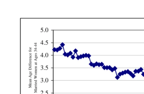
Figure 1: Mean Age Difference of Spouses by Birth Cohort.
Figure 1 shows that husbands tended to be almost 4.5 years older than their wives in the 1900 cohort, but just 2.5 years older by the 1950 cohort – today’s 52 year-olds. If the age gap does affect nursing home use, it must already have had an impact: all of the cohorts born between 1900 and 1920 have already begun to hit the ages when nursing home entry escalates (roughly 75 to 85 years old); across these cohorts, the age gap shrank by about half a year. As the more recent birth cohorts begin to hit these older ages, Figure 1 implies a potential for a large, ongoing effect on nursing home entry. Over 30 years, the age gap dropped from 3.5 years (for the 1920 cohort) to 2.5 years (for the 1950 cohort). Trends in the difference in the median age at first marriage for men versus women demonstrate a similar pattern (US Bureau of the Census 1998).
In this paper, we present a method for determining whether the nursing home population would have been larger than it is today had the age gap between spouses not declined. Moreover, we determine whether future nursing home demand will be lower than expected because of continued reductions in the age gap. Past research on long-term care has focused on the impact of changing longevity, aging of the population, social support, caregiving opportunities, nursing home prices, marital status, and disability (cf., Garber and MaCurdy 1990; Stern 1995). While our goal is to determine whether this additional factor – change in the spousal age gap – influences long-run changes in nursing home demand, our conclusions do not diminish the important role of
2.0 2.5 3.0 3.5 4.0 4.5 5.0
19021905 1908 1911 1914 1917 1920 1923 1926 192 9
193 2
193519381941 1944 1947 1950 1953
these other factors. In fact while our conclusions imply that the decline in the age gap will likely cause nursing home demand to be lower than expected, this effect will be offset by other factors and nursing home use will continue to increase substantially in the coming decades.
4. Methods
We investigate the effects of the changing age gap in three steps. First, using life table methods, we calculate the effect of the changing age difference on the risk of male and female widowhood. This allows us to calculate the change in the marriage rate—for different age and sex groups—that would have resulted from the changing difference in spousal ages. Second, we calculate the risk of nursing home entrance, conditional on age, sex, and marital status. Finally, we put the first two pieces of analysis together to calculate the effect of the age difference on nursing home entrance and the nursing home population.
We think of the entire population as broken up into various age-sex-marital status groups. The relative size of each group changes with the average age difference between spouses, as does the risk of nursing home entry faced by each group. Formally, therefore, we think of the nursing home population NH as depending on the average age difference X, according to:
( )
i( )
i( )
i
NH X
=
∑
N X p X
The number of people in each group, Ni, and the probability that a person in group i enters a nursing home, pi, both change with X. The total effect of changes in the age difference must account for its effect on the composition of the population and the risk of nursing home entry within each population group.
4.1. Age difference and the risk of widowhood
We start by assuming that each cohort enters age 65 with a total population of unity; we net out the effects of population trends by assigning all cohorts the same population size. From the Current Population Survey (an annual demographic survey whose sampling frame is based on the US Census), we calculate actual population shares by sex and marital status for each cohort at age 65. For example, if a cohort was observed to be 40 percent male and 60 percent female at age 65, we say that it enters age 65 with 0.4 males and 0.6 females. In addition, if married men in the cohort are on average
X
years older than their wives, each 65 year-old married man is assumed to have a65
−
X
year-old wife, and vice-versa.Define c t
MW as the number of married women in cohort c alive at age t in our
simulation. Similarly, define c t
MM as married men, c
t
SW as single women, and SMtc
as single men. Given values for 65
c
MW , MM , 65c
65
c
SW , and SM (calculated as in the65c
previous paragraph), each cohort is aged forward using life table data, as follows. Denote by S(a) the probability of surviving from age a to age a+1; cohort-specific survival curves are from the Social Security Administration (US Department of Health and Human Services 1992). We use different survival curves for men and women, but to economize on notation, we refer to a single one. The transition equations are given by: 1 1 1 1 [ ( ) ( ) ] [ ( ) ( ) ]
[ ( ) ] [ ( ) (1 ( ) ) ]
[ ( ) ] [ ( ) (1 ( ) ) ]
c c
t t
c c
t t
c c c
t t t
c c c
t t t
M W M W S t S t X
M M M M S t S t X
S W S W S t M W S t S t X
S M S M S t M M S t S t X
+ + + + = + = − = + − + = + − − (1)
Using the initial population estimates and the transition equations, we calculate for each cohort the steady-state population at each age-sex-marital status. Differences in these populations across cohorts will be influenced both by the changing age gap, X,
and by changes across cohorts in the probability of survival. Since we wish to focus on
the effect of age differences alone, we apply the survival curve of the 1955 cohort to all other cohorts. This eliminates differences in longevity across cohorts and focuses our attention on the impact of age differences alone.
4.2. Marriage and the risk of nursing home entry
The next step is to transform the effects on population into effects on the number of nursing home residents. We need to calculate the proportion of person-years spent in nursing homes for each age-sex-marital status cell. These proportions are then multiplied by the number of people in each cell to estimate the growth in the annual nursing home population. One way to recover these proportions is to estimate the probability that a person will spend the year in a nursing home. To accomplish this goal, we will specify a logistic model of nursing home entry.
Suppose that on any given day of his life, individual i faces a probability pi of spending that day in a nursing home, and a probability 1 – pi of spending it outside one. The advantages of this formulation are that it allows for exit from nursing home residence, and that it places more weight on people who are in nursing homes for a longer period of time. The disadvantage is that it treats each day in a nursing home as independent from the days preceding it. If person i lives for Di days, the likelihood of spending Ni of those days in a nursing home is given by piNi(1− pi)Di−Ni. A sample
of I individuals thus has the associated likelihood function:
,
)
1
(
)
(
1∏
= −−
=
I i N D i N i i i ip
p
L
(2)We will model
p
i as a logistic probability, where, ) exp( 1 ) exp( ’ ’ β β i i i X X p + =
and Xi is a column vector of characteristics for individual i.
Given the maximum likelihood parameters
β
, we estimate for every individual inprobability of nursing home entrance for each cell. This is equal to the expected proportion of people within each cell who will enter nursing homes. Applying this proportion to our estimates of the population within each cell, we can construct estimates of the nursing home population for each cohort and each cell.
4.2.1. Data
To estimate the probability of nursing home entry, we use data from the 1992-1996 Medicare Current Beneficiary Surveys (MCBS) Cost and Use Files. While data are available for 1997-99, they are not comparable to the earlier years, because of a difference in the way nursing home residents are asked about their disability status. By estimating the risk of nursing home entry in a single data set, we implicitly hold technology fixed at its 1990s levels to focus on the effects of the changing age gap. In practice, however, the risk of nursing home entry has remained a fairly stable function of age, marriage, and disability rates, even over periods of substantial change in the utilization of nursing homes and the availability of home health care and other alternatives to nursing homes (Lakdawalla and Philipson 2002).
The MCBS is a panel data set, every year of which is a weighted sample of the Medicare population. Since all individuals over age 65 are on Medicare, it can also be used as a nationally representative sample of individuals over 65; even though it is a panel, the sample is refreshed annually to correct for attrition and produce a nationally representative sample. Significantly, the MCBS samples all individuals, both institutionalized and non-institutionalized. The oldest-old (over 85 years of age) are oversampled. The MCBS collects age, sex, marital status, and disability status, where disability is measured as the number of limitations on Activities of Daily Living (ADL). There are six ADL limitations in total, which consist of difficulties with: bathing, dressing, eating, using the toilet, getting up from a chair, and walking.
in nursing homes were those who enter during the 8-year life of the panel. As a result, these data sets systematically understate the mean risk of nursing home admission. This problem is exacerbated by the fact that HRS/AHEAD often do not collect information on nursing home stays for people who die between waves of the survey: since nursing homes represent the last source of medical care for many terminally ill patients, this will further bias down estimates of nursing home risk. The MCBS, on the other hand, does report this information for decedents, either from administrative records or proxy interviews. Therefore, it allows us to construct an accurate estimate of nursing home risk. The key drawback of the MCBS is its nature as an individual-based survey, rather than a family-based survey. Therefore, we have very limited information on the spouses of respondents, and most significantly, we do not have data on spousal dates of birth. The HRS and AHEAD, on the other hand, do have some information on spousal ages, because they are family-based surveys. However, even for these data sets, spousal date of birth is available only for living spouses. We would have had to impute the information for deceased spouses. Since about 40% of the US population over age 65 is widowed, this is a significant issue. In sum, we chose the MCBS and its complete data on nursing home risk, over the HRS/AHEAD and its incomplete data on spousal ages. As a result, we impute spousal ages for the MCBS sample according to the procedure described below.
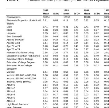
Annual summary statistics for the MCBS are presented in Table 1. The summary statistics are weighted in order to represent the entire population over the age of 65. The table indicates that 41 percent of the population is male, and the median age is around 75. Relatively few people have more than a high school education or more than $30,000 in annual income. About half are married, and over 30 percent have an ADL limitation of some kind. The prevalence of ADLs is a bit higher in the MCBS than in other surveys, primarily due to a difference in the question about walking limitations. The MCBS asks respondents if they have trouble walking 2-3 blocks, whereas other surveys (such as the National Health Interview Survey) tend to ask if they have trouble getting around inside their house. High blood pressure and heart disease are the most common ailments among the MCBS population. About half the population has been diagnosed with high blood pressure at some point in their lives, and roughly the same proportion has been diagnosed with heart disease.
Table 1: Annual Summary Statistics for the MCBS Population
1992 1993 1994 1995 1996
Mean St Dv Mean St Dv Mean St Dv Mean St Dv Mean St Dv
Observations 10554 10152 10516 9930 9823
Statewide Proportion of Medicaid Eligible
0.11 0.05 0.11 0.05 0.12 0.05 0.12 0.05 0.11 0.05
Male 0.41 0.49 0.41 0.49 0.41 0.49 0.41 0.49 0.41 0.49
Black 0.08 0.28 0.08 0.28 0.08 0.27 0.08 0.27 0.08 0.27
Hispanic 0.05 0.21 0.05 0.22 0.05 0.22 0.05 0.22 0.05 0.22
Ever Smoked? 0.58 0.49 0.60 0.49 0.62 0.49 0.62 0.49 0.62 0.49
Age 85 and Over 0.12 0.32 0.12 0.33 0.13 0.33 0.13 0.34 0.13 0.33
Age 80 to 84 0.14 0.34 0.14 0.34 0.14 0.35 0.14 0.35 0.15 0.35
Age 75 to 79 0.20 0.40 0.20 0.40 0.20 0.40 0.20 0.40 0.21 0.40
Age 70 to 74 0.25 0.44 0.26 0.44 0.27 0.44 0.26 0.44 0.28 0.45
Number of Children Living 2.68 2.26 2.74 2.27 2.78 2.25 2.81 2.26 2.80 2.24 Education less than High School 0.43 0.50 0.43 0.49 0.41 0.49 0.41 0.49 0.39 0.49 Education: Some College 0.13 0.34 0.13 0.34 0.14 0.34 0.14 0.35 0.15 0.35 Education: College Degree 0.08 0.28 0.08 0.28 0.08 0.28 0.09 0.28 0.09 0.29 Education: Post-College
Education
0.05 0.21 0.05 0.21 0.05 0.22 0.05 0.21 0.05 0.21
Married 0.54 0.50 0.56 0.50 0.56 0.50 0.53 0.50 0.53 0.50
Income: $10,000 to $30,000 0.50 0.50 0.51 0.50 0.50 0.50 0.51 0.50 0.52 0.50 Income: $30,000 to $50,000 0.11 0.31 0.12 0.32 0.13 0.34 0.13 0.34 0.14 0.35 Income: Above $50,000 0.05 0.21 0.05 0.22 0.05 0.22 0.06 0.24 0.07 0.26
ADLs=1 0.14 0.34 0.12 0.33 0.11 0.32 0.11 0.32 0.11 0.31
ADLs=2 0.07 0.25 0.07 0.25 0.07 0.25 0.06 0.24 0.06 0.24
ADLs=3 0.04 0.19 0.04 0.19 0.04 0.19 0.04 0.19 0.03 0.18
ADLs=4 0.03 0.17 0.03 0.17 0.03 0.17 0.03 0.17 0.03 0.16
ADLs=5 0.04 0.19 0.04 0.19 0.04 0.19 0.04 0.19 0.04 0.18
ADLs=6 0.04 0.19 0.04 0.19 0.04 0.19 0.04 0.19 0.04 0.20
High Blood Pressure 0.51 0.50 0.53 0.50 0.54 0.50 0.54 0.50 0.54 0.50
Heart Disease 0.42 0.49 0.44 0.50 0.44 0.50 0.44 0.50 0.42 0.49
Alzheimer’s Disease 0.04 0.20 0.05 0.21 0.05 0.22 0.05 0.22 0.06 0.23 Parkinson’s Disease 0.02 0.14 0.02 0.13 0.02 0.13 0.02 0.12 0.02 0.14
Stroke 0.11 0.31 0.12 0.32 0.12 0.33 0.13 0.33 0.13 0.33
Diabetes 0.16 0.37 0.17 0.38 0.18 0.38 0.17 0.38 0.16 0.37
Broken Hip 0.05 0.22 0.05 0.22 0.06 0.23 0.05 0.23 0.05 0.22
Emphysema 0.13 0.34 0.14 0.35 0.15 0.35 0.15 0.35 0.14 0.35
Cancer (except skin) 0.18 0.39 0.19 0.39 0.20 0.40 0.20 0.40 0.19 0.39 Partial Paralysis 0.07 0.26 0.07 0.26 0.07 0.26 0.06 0.24 0.06 0.23
Amputee 0.01 0.11 0.01 0.11 0.01 0.10 0.01 0.11 0.01 0.10
Osteoporosis 0.09 0.29 0.10 0.30 0.11 0.31 0.11 0.32 0.12 0.33
Psychological Disorders 0.04 0.20 0.05 0.21 0.05 0.22 0.05 0.22 0.05 0.22
questionnaire, and the data collected from it, forms the basis of the PUMS data set, which is available in every Census year. Since most demographic surveys (such as the Current Population Surveys, and National Health Interview Surveys) are based on the sampling information collected in the Census, the Census PUMS sample represents one of the most reliably representative samples, for use in detailed demographic analyses of the US population. It is the “gold standard” for analyses of population age structure and family composition in the US.
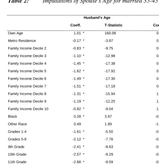
We constructed a sample of every married person in the 1960 PUMS, containing the variables: own age, spouse’s age, dummies for state of residence, a dummy for metropolitan residence status, dummies for family income decile, dummies for race (white, black, or other), dummies for educational attainment (no schooling, 1-4 years of schooling, 5-8 years of schooling, 9th grade, 10th grade, 11th grade, 12th grade, college attendee, and college graduate), and veteran status.
Table 2: Imputations of Spouse’s Age for married 35-45 year-olds in 1960 Census.
Husband’s Age Wife’s Age
Coeff. T-Statistic Coeff. T-Statistic
Own Age 1.01 * 160.08 0.90 * 162.15
Metro Residence -0.17 * -3.87 0.02 0.57
Family Income Decile 2 -0.83 * -9.75 0.19 * 2.63
Family Income Decile 3 -1.10 * -12.98 0.27 * 3.69
Family Income Decile 4 -1.45 * -17.38 0.52 * 7.31
Family Income Decile 5 -1.62 * -17.92 0.62 * 8.53
Family Income Decile 6 -1.49 * -17.30 0.86 * 11.64
Family Income Decile 7 -1.51 * -17.18 0.91 * 12.48
Family Income Decile 8 -1.31 * -15.94 1.08 * 14.56
Family Income Decile 9 -1.19 * -12.25 1.24 * 17.03
Family Income Decile 10 -0.82 * -9.04 1.27 * 15.90
Black 0.28 * 3.97 -0.26 * -4.27
Other Race 0.49 1.89 -1.57 * -7.15
Grades 1-4 -1.61 * -5.50 -0.74 * -3.38
Grades 5-8 -2.12 * -7.76 -0.68 * -3.27
9th Grade -2.41 * -8.63 -0.56 * -2.62
10th Grade -2.57 * -9.29 -0.48 -2.28
11th Grade -2.68 * -9.59 -0.60 * -2.80
12th Grade -3.12 * -11.45 -0.51 -2.46
College Attendee -3.25 * -11.73 -0.57 * -2.68
College Graduate -3.64 * -12.95 -0.94 * -4.43
Constant 7.31 * 18.69 -0.45 * -12.45
Veteran Status . . 1.24 * 3.86
Observations 87278 82879
R-Squared 0.251 0.268
Notes:
Dependent variable is age of spouse. T-statistics are robust *Significant at the 1% level.
4.2.2. Statistical model
Given the MCBS data and the imputed age of spouse, we estimate a logistic model:
1 2 3 4
*
5*
6i i i i i i i i i
X
′
β β β
= +
Age
+
β
Marr
+
β
Marr
∆ +
β
EvMarr
∆ +
Q
′
β ε
+
(3) The variables Marri and EvMarri are dummies for whether the individual is married or has ever been married. The age difference between spouses is ∆i, and is always
defined by the person’s own age minus the spouse’s age. Without loss of generality,
i
∆ is set to zero for the never-married.
β
2 measures the effect of age on the risk of nursing home entrance, and we expect it to be positive.β
3 measures the effect ofmarriage; to the extent that spouses function as a substitute for nursing home care, we expect it to be negative. (It is also possible that marriage signals better health: see e.g., Ebrahim, Wannamethee et al. 1995; Lillard and Panis 1996.)
β
4 measures the effect ofage difference for currently married people. If having a younger spouse affords better protection against nursing home entry, we expect it to be negative.
β
5, on the otherhand, measures the effect on ever-married people of the age difference, but controlling for observable health and marital status. We separate the effect of age differences for widowed and married people, because the age difference affects the availability of spousal care for married people, but not for widowed people. A married women with a very old husband may not be able to receive care from him as readily as one with a younger husband. A widowed woman, on the other hand, will not receive care from a spouse regardless of the age difference.
β
5 will pick up the indirect effect of agedifference on unobserved health, and it is identified by variation in spouse’s age among those who are widowed. This is not to say that
β
5 measures the overall effect ofhealth, only that portion of unobserved health that may be correlated with the age difference. Since these people no longer have a spouse, it is unaffected by the spouse’s ability to provide care at home, and represents instead a measure of the surviving spouse’s health. Finally, Qi represents a vector of other characteristics, including ADLs, sex, race, income category, and educational attainment.
An important simplification made by this model is the linearity of the age difference and marriage effects. A one-year increase in the age gap is presumed to have the same effect no matter what its starting point. This assumption was not found to affect our ultimate results of interest: we introduced squared and cubic terms in
i
are on the composition of the population, rather than on its risk of nursing home entry. We also assume that the effect of marriage itself is linear. The coefficient
β
3 measuresthe difference in risk between a never married person and a married person whose spouse is of identical age. It is the effect of marriage abstracting from any spousal age difference. Linearity means this effect is assumed to be the same for those with older (or younger) spouses as it is for those with identically aged spouses. We tested the robustness of this assumption by creating one-year categorical variables for the age difference (i.e., there was a dummy variable for a difference of –2, one for a difference of –1, one for a difference of zero, and so on) and fully interacting these with the marriage variable. We found similar results with this more flexible specification.
Finally, due to data constraints, the model makes some other simplifications by ruling out the effect of nursing home prices, abstracting from interactions among disease conditions, and abstracting from the possibility that some people are so sick that they die before entering a nursing home. Recognizing these limitations, we perform sensitivity analysis in Section 5.3 designed to show the possible impact of errors in estimating the risk of nursing home entrance.
4.3. Age difference and the nursing home population
The final step is to calculate the size of the nursing home population for each cohort, and each marital status cell. Given the size of the population in each age-sex-marital status cell, it remains only to calculate the risk of nursing home entrance. To do this, we assume that, within an age-sex-marital status cell, every cohort is identical to the MCBS sample in every respect, except in its age difference between spouses. Therefore, to calculate the risk of nursing home entrance for a particular cohort c, that has an average age difference X, we keep the MCBS sample as is, but we assign every ever-married person in it the age difference X. Using these characteristics, we then compute the average risk of nursing home entrance within an age-sex-marital status cell. This represents the cell-specific risk of nursing home entrance that cohort c would face as a result of its age difference X, and holding all other characteristics constant at their MCBS levels.
We multiply these cell-specific risks by the cohort’s cell-specific population; this yields the cell-specific nursing home population. To understand this procedure more formally, let
smt
simulations described in Section 4.1. The entrance probabilities also depend on the age gap, as well as other characteristics of the cell, such as its average disability, race, and
so on. We will refer to these other characteristics using the vector
Y
v
, which represents the characteristics of the MCBS population. These definitions allow us to write the nursing home population as a function of the age gap between spouses:, ,
(
c)
smt(
c)
smt(
c; )
s m t
NH X
=
∑
N
X
p
X Y
v
(4)
Equation 4 demonstrates the relationship between the nursing home population and the age gap between spouses.
5. Results
5.1. Age difference and the risk of widowhood
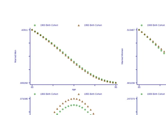
Figure 2: Projected Effect of Age Differences on the Married and Unmarried Populations
The declining age gap means that women find themselves married to relatively younger men. Therefore, as Figure 2 shows, across cohorts, the population of married women rises by 6.13 percent; the unmarried female population falls by 6.80 percent; the married male population falls by 2.45 percent; and the unmarried male population rises by 8.96 percent. We will see that, given the size of the relationship between marriage and nursing home risk, these changes have significant impacts on nursing home populations and total nursing home expenditures.
5.2. Marriage and the risk of nursing home entry
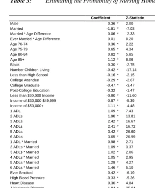
Section 4.2. presented our methods for estimating the effect of population changes on the nursing home population. Table 3 presents the associated results of our maximum likelihood estimation procedure. The table shows coefficients, robust z-statistics, and marginal effects for each variable. The marginal effect is computed as the average marginal effect for each individual in the data set and should be interpreted as the expected value of the marginal effect. As expected, married people are less likely to
Mar
ri
ed Men
age
1900 Birth Cohort 1955 Birth Cohort
65 95 .005292 .42911 Mar ri ed W o men age
1900 Birth Cohort 1955 Birth Cohort
65 95 .001239 .513487 U n mar ri ed Men age
1900 Birth Cohort 1955 Birth Cohort
65 95 .018303 .071095 U n mar ri ed W o men age
1900 Birth Cohort 1955 Birth Cohort
65 95
enter nursing homes, and the effect of marriage is stronger for those with younger spouses. However, the effect of marriage is attenuated for highly disabled people, according to the interaction terms between ADLs and marriage. This is understandable, since it is harder for a spouse to care for a highly disabled mate than a less disabled one. In keeping with the importance of alternative caregivers, people who have more living children are less likely to enter a nursing home. The effect of spouse’s age difference on those who have ever been married, on the other hand, is negligible. Of course, since we were forced to impute our data on age difference, our evidence on this point should not be taken as conclusive. In addition, the probability of nursing home entrance goes down with income—probably because income is correlated with unobserved health, and because elderly people spend down their assets in order to become eligible for Medicaid—and it goes up with disability and disease.
Table 3: Estimating the Probability of Nursing Home Entry in the MCBS.
Coefficient Z-Statistic Marginal Effect
Male 0.36 * 2.00 0.0090
Married -1.81 * -7.03 -0.0449
Married * Age Difference -0.06 * -2.33 -0.0014
Ever Married * Age Difference 0.01 0.20 0.0001
Age 70-74 0.36 * 2.22 0.0089
Age 75-79 0.65 * 4.34 0.0161
Age 80-84 0.82 * 5.85 0.0202
Age 85+ 1.12 * 8.06 0.0278
Black -0.30 * -2.75 -0.0075
Number Children Living -0.42 * -17.14 -0.0105
Less than High School -0.16 * -2.15 -0.0039
College Attendee -0.29 * -2.67 -0.0072
College Graduate -0.47 * -3.47 -0.0117
Post-College Education -0.32 -1.47 -0.0079
Less than $30,000 Income -0.80 * -11.60 -0.0199
Income of $30,000-$49,999 -0.87 * -5.39 -0.0216
Income of $50,000+ -1.11 * -4.48 -0.0275
1 ADL 1.09 * 7.43 0.0271
2 ADLs 1.90 * 13.81 0.0472
3 ADLs 2.42 * 16.67 0.0600
4 ADLs 2.41 * 16.72 0.0597
5 ADLs 3.42 * 26.60 0.0849
6 ADLs 3.65 * 26.99 0.0905
1 ADL * Married 0.98 * 2.71 0.0242
2 ADLs * Married 1.09 * 3.37 0.0271
3 ADLs * Married 1.02 * 2.86 0.0254
4 ADLs * Married 1.05 * 2.95 0.0261
5 ADLs * Married 1.29 * 4.27 0.0320
6 ADLs * Married 1.46 * 5.10 0.0363
Ever Smoked -0.42 * -6.19 -0.0105
High Blood Pressure -0.33 * -5.26 -0.0081
Heart Disease 0.30 * 4.84 0.0076
Alzheimer’s Disease 1.84 * 25.04 0.0456
Parkinson’s Disease -0.03 -0.17 -0.0006
Stroke 0.30 * 4.05 0.0075
Diabetes 0.10 1.37 0.0025
Hip Fracture 0.49 * 6.69 0.0121
Emphysema -0.01 -0.08 -0.0002
Cancer 0.05 0.72 0.0013
Partially Paralyzed 0.32 * 3.73 0.0079
Amputee -0.59 * -2.71 -0.0146
Osteoparosis -0.75 * -9.05 -0.0185
Psychological Disorder 1.03 * 11.28 0.0255
Constant -4.57 * -22.92 -0.1135
Notes:
Z-statistics are robust.
Using the coefficients in Table 3, we can now calculate the average risk of nursing home entrance within age-sex-marital status cells, by calculating the risk of entrance for each individual, and then averaging these risks within age-sex-marital status cells. This then allows us to determine how many married and unmarried men and women would require nursing home care, given the current state of health technology. It is worth emphasizing again that by estimating the risk of nursing home entrance from a 1990s data set, we are holding fixed health technology at its recent level, and removing it as a factor in determining nursing home demand.
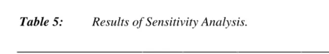
5.3. Age difference and the nursing home population
For each cohort c, Table 4 summarizes the quantity 1 9 0 0
1 9 0 0
( ) ( )
( ) c
N H X N H X
N H X
− , the
Table 4: The effect of the changing age difference of spouses on nursing home populations and expenditures
Percentage Change in Nursing Home Population Absolute Change in Nursing Home Expenditures ($millions)
Females Males Females Males
Married Unmarried All Married Unmarried All Married Unmarried All Married Unmarried All
0.0% 0.0% 0.0% 0.0% 0.0% 0.0% 0 0 0 0 0 0
2.5% -0.6% -0.3% -0.8% 1.2% 0.4% 115 -301 -186 -61 146 85
7.7% -1.9% -0.8% -2.7% 3.9% 1.2% 356 -928 -572 -193 461 268
9.3% -2.3% -1.0% -3.2% 4.8% 1.5% 433 -1,128 -695 -235 561 326
10.6% -2.7% -1.1% -3.7% 5.4% 1.7% 493 -1,283 -790 -266 636 370
9.7% -2.5% -1.0% -3.4% 5.0% 1.6% 453 -1,179 -726 -245 586 341
12.1% -3.0% -1.3% -4.1% 6.1% 1.9% 560 -1,456 -896 -301 719 418
15.4% -3.9% -1.6% -5.2% 7.8% 2.5% 717 -1,858 -1,141 -382 912 530
18.8% -4.7% -2.0% -6.4% 9.5% 3.0% 874 -2,257 -1,384 -466 1,113 647
18.4% -4.6% -1.9% -6.3% 9.2% 2.9% 852 -2,203 -1,350 -455 1,086 631
Note:
Expenditure changes are based on annual nursing home expenses of $50,000 per year, and 1997 nursing home populations from the MCBS of 92,869 married women, 145,485 married men, 960, 409 unmarried women, and 234,856 unmarried men.
From the 1900 to the 1955 birth cohorts the age gap fell from 4.43 to 2.61 years. The analysis implies that nursing home expenditures by women fell by $1.35 billion as a result of their spouses being 1.82 years younger. On the other hand, nursing home expenditures by men rose by $0.63 billion a result of their spouses being 1.82 years older. Of course, more married women entered nursing homes as a result of this, primarily because the number of married women grew. However, this was more than offset by the reduction of nursing home utilization by unmarried women. On the other hand, fewer married men entered nursing homes, because there were fewer married men around, but this was more than offset by growth in the entrance of unmarried men.
and married people equally. The last two columns show that decreasing the nursing home risk of married people would raise our estimated effect of the age gap by about 25%, while increasing this risk would lower it by about the same. Recall that our model overstated the risk for married people by about ten percent; the sensitivity analysis inflates their risk by twice that amount.
Table 5: Results of Sensitivity Analysis.
Base Case
Increased NH Risk for All
Decreased NH Risk for All
Increased NH Risk for Married
Decreased NH Risk for Married
Male Resident Change 1.00 1.00 1.00 0.79 1.25
Female Resident Change 1.00 1.00 1.00 0.77 1.24
Total Resident Change 1.00 1.00 1.00 0.76 1.24
Note:
Sensitivity analysis alters the forecasted Nursing Home risk for the stated population each population group by twenty percent, either upwards or downwards as indicated.
6. Discussion
Although on average husbands are still older than their wives, the average age gap has shrunk. As a result, women are less likely to enter nursing homes, while men are more likely to enter them. In terms of current dollars and health care technology, the 1955 birth cohort is likely to spend more than half a billion dollars less on nursing homes annually than the 1900 birth cohort simply because of the reduction in the age gap of spouses. Women in the younger cohort will spend $1.35 billion less, while men will actually increase their spending by more than $0.60 billion. As the age gap continues to decline (as depicted in Figure 1), nursing home expenditures may not rise as much as otherwise anticipated. While this factor should be included when making projections of nursing home demand, the effects are modest in relationship to the rise in nursing home demand resulting from the increasing number of people reaching old age.
poverty among the elderly, these changes could also affect welfare receipt and other public programs.
7. Acknowledgement
This research was supported by the National Institute on Aging, R03 AG19900.
Changes
On July 28th 2003, per request of the author, the following change was made:
On page 279, the sentence "We estimate that the decline in the difference in ages between spouses that took place between the birth cohorts of 1900 and 1955 may raise women’s annual nursing home expenditures by about $1.4 billion, but lower men’s expenditures by about $600 million."
was changed to:
References
Bergstrom, T. C. and M. Bagnoli (1993). "Courtship as a Waiting Game." Journal of Political Economy 101(1): 185-202.
Clark, S. C. (1995). "Advance Report on Final Marriage Statistics, 1989 and 1990." Monthly Vital Statistics Report 43(12).
Ebrahim, S., G. Wannamethee, et al. (1995). "Marital Status, Change in Marital Status, and Mortality in Middle-Aged British Men." American Journal of Epidemiology 142(8): 834-842.
Ettner, S. (1994). "The Effect of the Medicaid Home Care Benefit on Long-Term Care Choices of the Elderly." Economic Inquiry 32(1): 103-127.
Foley, D. J., A. M. Ostfeld, et al. (1992). "The Risk of Nursing Home Admissions in Three Communities." Journal of Aging and Health 4: 155-173.
Freedman, V. A., L. F. Berkman, et al. (1994). "Family Networks: Predictors of Nursing Home Entry." American Journal of Public Health 84: 843-845.
Garber, A. M. and T. MaCurdy (1990). Predicting Nursing Home Utilization Among the High-Risk Elderly. Issues in the Economics of Aging. D. A. Wise. Chicago, University of Chicago Press: 173-200.
Kemper, P. and C. Murtaugh (1991). "Lifetime Use of Nursing Home Care." New England Journal of Medicine 324: 595-600.
Lakdawalla, D. N. and T. J. Philipson (2002). "The Rise in Old-Age Longevity and the Market for Long-Term Care." American Economic Review 92(1): 295-306.
Lillard, L. A. and C. W. A. Panis (1996). "Marital Status and Mortality: The Role of Health." Demography 33(3): 313-327.
Norton, E. C. (1995). "Elderly Assets, Medicaid Policy, and Spend-Down in Nursing Homes." Review of Income and Wealth 41(3): 309-29.
OECD (1998). OECD Health Data 98: A Comparative Analysis of 29 Countries, OECD Electronic Publications.
Pezzin, L. E., P. Kemper, et al. (1996). "Does Publicly Provided Home Care Substitute for Family Care?" Journal of Human Resources 31(3): 650-676.
Steinbach, U. (1992). "Social Networks, Institutionalization, and Mortality Among Elderly People in the United States." Journal of Gerontology: Social Sciences 47: S183-S190.
Stern, S. N. (1995). "Estimating Family Long-Term Care Decisions in the Presence of Endogenous Child Characteristics." Journal of Human Resources 30(3): 551-80.
United States Congress Ways and Means Committee (2000). Green Book. Washington, DC, Government Printing Office.
US Bureau of the Census (1998). Marital Status and Living Arrangements: Match 1998 (Update). Washington, DC, US Bureau of the Census.