Population based algorithms for approximate optimal distributed control of wave equations

Vol 4, No. 2, (2014), pp 31-41

Population based algorithms for

approximate optimal distributed

control of wave equations

A. H. Borzabadi∗, S. Mirassadi and M. Heidari

Abstract

In this paper, a novel hybrid iterative scheme to find approximate optimal distributed control governed by wave equations is considered. A partition of the time-control space is considered and the discrete form of the problem is converted to a quasi assignment problem. Then a population based al-gorithm, with a finite difference method, is applied to extract approximate optimal distributed control as a piecewise linear function. A convergence analysis is proposed for discretized form of the original problem. Numerical computations are given to show the proficiency of the proposed algorithm and the obtained results applying two popular evolutionary algorithms, genetic and particle swarm optimization algorithms.

Keywords: Optimal control problem; Evolutionary algorithm; Finite differ-ence method; Wave equation

1 Introduction

In the past few decades, the science and engineering have witnessed a phe-nomenal growth in the field of optimal control problems (OCPs) governed by partial differential equations (PDEs), specially parabolic and hyperbolic equations. A large part of these improvements is due to the efforts of pioneer researchers such as J. L. Lions [15, 16, 17] and D. L. Russell [19, 20].

In particular, the controllability in wave equations are studied in [21, 22]. Kim and Erzberger [14] derived Riccati equation for optimum boundary

con-∗_{Corresponding author}

Received 24 December 2013; revised 17 May 2014; accepted 23 June 2014 A. H. Borzabadi

School of Mathematics and Computer Science, Damghan University, Damghan, Iran. Email: [email protected], [email protected]

S. Mirassadi

School of Mathematics and Computer Science, Damghan University, Damghan, Iran. M. Heidari

School of Mathematics and Computer Science, Damghan University, Damghan, Iran.

trol of wave equation, with quadratic cost function. Applicability of Laplace transform for determination of time optimal control for hyperbolic class of problems has been shown in [10]. But solving optimal control problems gov-erned by wave equations with analytical approaches, have some difficulties such as computing gradient, integrals in hyperbolic and parabolic equations and target functionals. For overcoming complexities due to the analytical ap-proaches, the numerical approaches are created based on various techniques as regularization [9, 8, 11], measure theoretical concepts [1, 5, 6] and penalty method [12].

Recently, nature-inspired optimization methods have attracted more and more attention and these powerful tools have been applied for solving a wide range of OCPs [2, 3, 7].

In this paper, by combinating one of the population based algorithms (Evolutionary Algorithms (EAs)) and a numerical method for solving wave equations (finite difference method), an effective numerical scheme for finding approximate optimal control and state functions has been procreated for OCPs governed by wave equations with a distributed control and a non-classical boundary condition as follows:

minimize J(ν(., .)) =

∫ T

0

∫ L

0

Φ(t, x, ν(x, t))dx dt (1)

subject to utt(x, t) =uxx(x, t) +ν(x, t), (x, t)∈[0, L]×[0, T] (2)

u(x,0) =φ(x), ut(x,0) =ψ(x), x∈[0, L] (3)

u(0, t) =µ(t), ux(L, t)−ux(0, t) =η(t), t∈[0, T] (4)

where φ(x), ψ(x), µ(t), η(t) are given functions andν(x, t) is a bounded dis-tributed control and gets its values in the intervalV ⊂R. The purpose is to find the approximate optimal controlν(x, t) and stateu(x, t) that minimize the functional (1) and satisfy the wave equation (2) with initial conditions (3), boundary conditions (4) and terminal conditions

u(x, T) =ω(x), ut(x, T) =ζ(x). (5)

Hereω(x) andζ(x) are target functions.

2 Description of the method

To find the optimal solution we must examine the performance index in the set of all possibilities of control-state pairs. The set of admissible pairs con-sisting of pairs like (u, ν) satisfying in (2)-(4) is denoted byP. In this section we consider a control space discretization based method considering equidis-tant partitions of [0, T], [0, L] andV as △t={0 =t0, t1,· · · , tn−1, tn =T} △x ={0 = x0, x1,· · ·, xm₋1, xm = L} and △ν = {v0, v1,· · ·, vl₋1, vl},

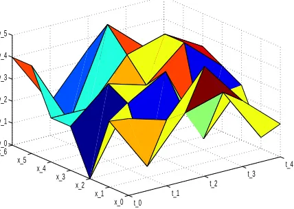
re-spectively. Now the main problem can be considered as a quasi assignment problem, where a performance index can be assigned corresponding to each chosen partition and choosing the best performance index can lead to deter-mine the near optimal control of the problem. A trivial way to deterdeter-mine the near optimal solution is to calculate all possible partitions and compare the corresponding trade offs. This trivial method of total enumeration needs ((m+ 1)(n+ 1))(l+1) evaluation. A typical discretization is given in Figure

t_0 t_1

t_2 t_3

t_4

x_0 x_1 x_2 x_3 x_4 x_5 x_6 v_0 v_1 v_2 v_3 v_4 v_5

Figure 1: A typical control function in time-control space

1 with n = 4, m = 6 and l = 5. To avoid so many computations, we use the EAs for evaluating special partitions that guides us to the optimal one. For each partition of control we need its corresponding trajectory to evaluate the performance index. Trivially, the corresponding trajectory should be in discretized form.

uj_i−1−2uj_i +uj_i+1

k2 =

uj_i+1−2uj_i +uj_i−1

h2 + ¯ν

j i,

u0_i =φi,

u1

i −u

0

i

k =ψi, uj₀=µj,

uj_m+1−uj m

h −

uj₁−uj₀

h =η

j_,

where uj_i = u(xi, tj), φi = φ(xi), ψi = ψ(xi), µj = µ(tj), ηj = η(tj) and ¯

νj_i = ¯ν(xi, tj).Then we have

u0_i =φi, u1i =kψi+u0i, i= 0,1,· · ·, m, (6)

uj₀=µj, u j

m+1=hη

j_+uj m+u

j

1−u

j

0, j= 0,1,· · ·, n, (7)

and

uj_i+1=λ2uj_i+1+ (2−2λ2)uj_i+λ2uj_i−1−u_ij−1+k2ν¯_ij, (8) wherej = 1,2,· · ·, n, i= 0,1,· · · , mandλ=k/h.

If (u,ν¯) be a pair of the trajectory and the control which satisfies in (10)-(11) and

∥u(xi, tn)−ω(xi)∥ ≤ϵ1 i= 0,1,· · ·, m (9)

∥ut(xi, tn)−ζ(xi)∥ ≤ϵ2 i= 0,1,· · ·, m (10)

for given small numbersϵ1 >0 and ϵ2>0, then we can claim that, a good

approximate pair for minimizing functional J in (1) has been found. Here ∥ · ∥is the infinity norm.

Also in (1), the integral term can be estimated by a numerical method of integration, e.g. one of Newton-Cotes methods. After discretization of the OCP governed by wave equation, the problem is converted to opti-mization problem with two extra objective functions. We add the terms,

∑m−1

i=1 ∥u(xi, tn)−ω(xi)∥ and

∑m−1

i=1 ∥ut(xi, tn)−ζ(xi)∥ to the original

ob-jective function and then, we apply EAs for this new criteria function. There-fore, by applying the above method, the OCP governed by wave equation is converted to constrained programming:

(CP) min m ∑ i=1 n ∑ j=1

AiBjΦ(tj, xi,ν¯ij) (11)

+M

m

∑

i=1

∥uni −ω(xi)∥+W m

∑

i=1

subject to uj_i+1=λ2uj_i+1+ (2−2λ2)uj_i+λ2uj_i−1−u_ij−1+k2ν¯_ij, (12)

u0_i =φi, u1i =kψi+u0i, i= 0,1,· · ·, m, (13)

uj₀=µj, u j

m+1=hη

j_+uj m+u

j

1−u

j

0, j= 0,1,· · ·, n, (14)

where, Ai and Bj are the weights of a numerical method of integration, M and W are large positive numbers (as the parameters in penalty function approach).

3 Convergence

The solution of (CP) approximates the original problem by minimizing

J(u, ν) over the subset PN of P consists of all piecewise linear functions

u(., .) and ν(., .) with nodes atuj_i,ν¯_ij, j= 0,1,· · ·, N, i= 0,1,· · ·, N which satisfies (11) and the objective function (11) for this nodes called JN, here without loss of generality, we assume that N =m =n. Our first aim is to show that P1⊆ P2⊆ P3· · · in an embedding fashion.

Lemma 1. There exists an embedding that maps PN to a subset of PN+1

for allN = 1,2,· · ·.

Proof. For simplicity, we prove the case whenN = 1. The proof forN ≥2 is obtained analogously.

Let consider an arbitrary pair (u, ν) inP1 represented byu

j i,ν¯

j

i, j= 0,1, i= 0,1. We have to find a corresponding pair (ˆu,νˆ) in P2 with ˆu

j i,νˆ¯

j i, j = 0,1,2, i= 0,1,2,as nodes that corresponds to (u, ν). We have from (11)

uj_i+1=λ2uj_i+1+ (2−2λ2)uj_i+λ2u_ij₋₁−uj_i−1+k2ν¯_ij, j= 0,1, i= 0,1,

where uj_i+1=u(xi, tj+1). On the other hand, a typical element (ˆu,νˆ) in P2

satisfies

ˆ

uj_i+1=λ2uˆj_i+1+ (2−2λ2)ˆuj_i+λ2uˆj_i−1−uˆj_i−1+k2νˆ¯_ij, j= 0,1,2, i= 0,1,2,

where ˆuj_i+1= ˆu(ˆxi,ˆtj+1).

It is clear that here we have ˆxi =xi, i= 0,1 and ˆtj =tj, j= 0,1.Therefore we can choose ˆuj_i,νˆ¯_ij, j= 0,1,2, i= 0,1,2 in such a way that

ˆ

uj_i =uj_i, j= 0,1, i= 0,1.

This shows that the constructed pair (ˆu,νˆ) corresponds to (u, ν) and belongs toP2.

Theorem 1. If µN = infPNJN for N = 1,2,· · ·, and µ∗ = infPJ exists, thenlimN→∞µN =µ∗.

Proof. By Lemma 1, we haveµ1 ≥µ2 ≥ · · · ≥ µ∗. So, this decreasing and

bounded sequence converges to a limit µ0 _≥µ∗_{. It is enough to show that}

µ0_=µ∗_{. Ifµ}0_{> µ}∗_{, thenϵ=µ}0_−µ∗_{>0 and by continuity ofJ(u, ν), we may}

find a pair (uj n0, ν

j

n0),such that|J(u

j n0, ν

j n0)−µ

∗_{|< ϵ,thenJ(u}j n0, ν

j n0)< µ

0_,

and so µn0 < µ

0 _{which is incorrect and thereforeµ}0_=µ∗_.

4 Algorithm of the approach

In this section, an algorithm on the basis of the previous discussions is pre-sented. This algorithm is designed in two stages, initialization step and main steps, where the main steps contain the main structure of algorithm consid-ering initialization step.

Initialization step:

Choose an equidistant partition for time interval [0, T], with parameter dis-cretizationk=tj+1−tj, j= 0,1,· · · , n−1 and an equidistant partition for interval [0, L], with parameterh=xi+1−xi, i= 0,1,· · · , m−1.

Main steps:

Step 1. Choose a population randomly.

Step 2. Computeuj_i, j= 0,1,· · ·, n, i= 0,· · ·, m, using (10)-(11).

Step 3. Fitness scores are assigned to each population using objective func-tion of (CP).

Step 4. Apply the rules of EA for current population.

Step 5. Consider the new population as the current population.

Step 6. If the termination conditions are satisfied, stop; otherwise jump to Step 2.

5 Numerical results

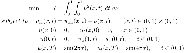
In this section the proposed algorithm in the previous section is examined by one numerical example. We have applied PSO and GA as two of the most popular EAs.

min J =

∫ 1

0

∫ 1

0

ν2(x, t)dt dx

subject to utt(x, t) =uxx(x, t) +ν(x, t), (x, t)∈(0,1)×(0,1)

u(x,0) = 0, ut(x,0) = 0, x∈(0,1)

u(0, t) = 0, ux(1, t) =ux(0, t), t∈(0,1)

u(x, T) = sin(2πx), ut(x, T) = sin(4πx), t∈(0,1)

For analytical solution of this example, see [13].

Our solutions by P SO and GA algorithms are shown in the following tables:

• where wave parameters, λ, be 0.1,0.2,0.3,0.4,0.5,0.6,0.7,0.8,0.9,1.0 and the population sizes, (m), be 200 and the number of iterations,(kmax), be 500, results are shown in Table 1. 1.

• where the population size,(m), be 50,100,150,200,250,300,350 and the number of iterations,(kmax), be 500 and parameter wave equation,λ, be 0.2, results are shown in Table 2. 2.

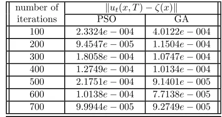
• where the number of iterations,(kmax), be 100,200,300,400,500,600,700 and the population size,(m), be 200 and parameter wave equation,λ, be 0.2, results are shown in Table 3. 3.

Also comparison betweenω(x) andζ(x) withu(x, T) andut(x, T) are shown in Figures 2 and 3 ,respectively, whenm= 200, kmax= 500, λ= 0.2.

Table 1: Comparison of the errors due to applying PSO and GA with increasingλ parameter ∥ut(x, T)−ζ(x)∥

λ PSO GA

Table 2: Comparison of the errors due to applying PSO and GA with increasing the number of population

number of ∥ut(x, T)−ζ(x)∥

population PSO GA

50 1.8470e−004 2.16684e−004 100 1.1513e−004 9.4944e−005 150 1.5074e−004 1.0690e−004 200 9.4195e−005 8.5366e−005 250 1.6513e−004 1.2451e−004 300 1.6264e−004 1.0645e−004 350 5.0556e−005 8.6299e−005

Table 3: Comparison of the errors due to applying PSO and GA with increasing the number of iterations

number of ∥ut(x, T)−ζ(x)∥

iterations PSO GA

100 2.3324e−004 4.0122e−004 200 9.4547e−005 1.1504e−004 300 1.8058e−004 1.0747e−004 400 1.2749e−004 1.0134e−004 500 2.1751e−004 9.1401e−005 600 1.0138e−004 7.7138e−005 700 9.9944e−005 9.2749e−005

6 Conclusion

0 0.2 0.4 0.6 0.8 1 −1

−0.8 −0.6 −0.4 −0.2 0 0.2 0.4 0.6 0.8 1

x

ut

(x,T)

Exact u

t(x,T)

PSO u_t(x,T) GA u_t(x,T)

Figure 2: Diagram ofu(x, T) andω(x)

0 0.2 0.4 0.6 0.8 1

−1.5 −1 −0.5 0 0.5 1

x

u(x,T)

Exact u(x,T) PSO u(x,T) GA u(x,T)

Figure 3: Diagram ofut(x, T) andζ(x)

References

1. Alavi, S.A., Kamyad, A.V. and Farahi, M.H. The optimal control of an inhomogeneous wave problem with internal control and their numerical solution, Bulletin of the Iranian Mathematical society 23(2) (1997) 9-36.

2. Borzabadi, A.H. and Mehne, H. H. Ant colony optimization for optimal

(2009) 259-264.

3. Borzabadi, A.H. and Heidari, M. Comparison of some evolutionary algo-rithms for approximate solutions of optimal control problems, Australian Journal of Basic and Applied Sciences, 4(8) (2010) 3366-3382.

4. Borzabadi, A.H. and Heidari, M.Evolutionary algorithms for approximate optimal control of the heat equation with thermal sources, Journal of Math-ematical Modelling and Algorithms, DOI: 10.1007/s10852-011-9166-0. 5. Farahi, M.H., Rubio, J.E. and Wilson, D.A. The Optimal control of the

linear wave equation, International Journal of control, 63 (1996) 833-848. 6. Farahi, M.H., Rubio, J.E. and Wilson, D.A.The global control of a non-linear wave equation, International Journal of Control 65(1) (1996) 1-15. 7. Fard, O.S. and Borzabadi, A.H. Optimal control problem,

quasi-assignment problem and genetic algorithm, Enformatika, Transaction on

Engin. Compu. and Tech., 19 (2007) 422 - 424.

8. Gerdts, M., Greif, G. and Pesch, H.J. Numerical optimal control of the wave equation: Optimal boundary control of a string to rest in finite time, Proceedings 5th Mathmod Vienna, February (2006).

9. Glowinski, R., Lee, C.H. and Lions, J.L. A numerical approach to the exact boundary controllability of the wave equation (I) Dirichlet controls: description of the numerical methods,Japan J. Appl. Math., 7 (1990) 1-76. 10. Goldwyn, R.M., Sriram, K.P. and Graham, M.H. Time optimal control of a linear hyperbolic system, International Journal of Control, 12 (1970) 645-656.

11. Gugat, M., Keimer, A. and Leugering, G.Optimal distributed control of the wave equation subject to state constraints, ZAMM . Z. Angew. Math. Mech. 89(6) (2009) 420-444.

12. Gugat, M.Penalty techniques for state constrained optimal control prob-lems with the wave equation, SIAM J. Control Optim. 48 (2009) 3026-3051. 13. Hasanov, K.K. and Gasumov, T.M.Minimal energy control for the wave

equation with non-classical boundary condition, Appl. Comput. Math.,

9(1) (2010) 47-56.

14. Kim, M. and Erzberger, H.On the design of optimum distributed param-eter system with boundary control function, IEEE Transactions on Auto-matic Control, 12(1) (1967) 22-28.

16. Lions, J.L. Some aspect of the optimal control of distributed parameter systems, SIAM, Philadelphia, 1972.

17. Lions, J.L. Exact controllability stabilization and perturbations for dis-tributed systems, SIAM Rev., 30 (1988) 1 - 68.

18. Rubio, J.E.Control and optimization; the linear treatment of non-linear problems, Manchester, U. K., Manchester University Press, 1986.

19. Russell, D.L.A unified boundary controllability theory for hyperbolic and parabolic partial differential equations, Studies in Appl. Math., 52 (1973) 189-211.

20. Russell, D.L. Controllability and stabilizability theory for linear partial differential equations: recent progress and open questions, SIAM Rev., 20(4) (1979) 639-739.

21. Zuazua, E. Exact controllability for the semilinear wave equation, J. Math. Pures Appl., 69(1990) 1-31.

جﻮﻣ تﻻدﺎﻌﻣ ﺖﺤﺗ ﯽﻌﯾزﻮﺗ ﻪﻨﯿﻬﺑ لﺮﺘﻨﮐ ﺐﯾﺮﻘﺗ یاﺮﺑ ﺖﯿﻌﻤﺟ ﻪﯾﺎﭘ ﺮﺑ ﯽﻤﺘﯾرﻮﮕﻟا

یرﺪﯿﺣ ﺪﻤﺤﻣ و ،یﺪﺳاﺮﯿﻣ ﻢﮕﯿﺑ ﻪﻨﯿﮑﺳ ،یدﺎﺑآزﺮﺑ ﯽﻤﺷﺎﻫ ﺮﺒﮐا

ﺮﺗﻮﯿﭙﻣﺎﮐ و ﯽﺿﺎﯾر مﻮﻠﻋ هﺪﮑﺸﻧاد ،نﺎﻐﻣاد هﺎﮕﺸﻧاد

ﻪﻟدﺎﻌﻣ ﺖﺤﺗ ﯽﻌﯾزﻮﺗ ﯽﺒﯾﺮﻘﺗ ﻪﻨﯿﻬﺑ لﺮﺘﻨﮐ ﻦﺘﻓﺎﯾ یاﺮﺑ ﻦﯾﻮﻧ یراﺮﮑﺗ ﯽﻘﯿﻔﻠﺗ شور ﮏﯾ ،ﻪﻟﺎﻘﻣ ﻦﯾا رد: هﺪﯿﮑﭼ