in the population sciences published by the Max Planck Institute for Demographic Research Konrad-Zuse Str. 1, D-18057 Rostock·GERMANY www.demographic-research.org
DEMOGRAPHIC RESEARCH
VOLUME 14, ARTICLE 6, PAGES 85-110
PUBLISHED 14 FEBRUARY 2006
http://www.demographic-research.org/Volumes/Vol14/6/ DOI: 10.4054/DemRes.2006.14.6
Research Article
Demographic translation and tempo effects:
An accelerated failure time perspective
Germán Rodríguez
c
1 Introduction 86
2 Fertility 87
2.1 Translating fertility 88
2.2 Tempo-adjusted fertility 89
2.3 A synthetic cohort interpretation 91
2.4 Cohort and period shifts 94
3 Mortality 95
3.1 Mortality translation 96
3.2 The Bongaarts-Feeney model 97
3.3 Four measures of longevity 99
3.4 Cohort survival 101
3.5 A proportional hazards models 104
4 Discussion 106
5 Acknowledgements 108
Demographic translation and tempo effects:
An accelerated failure time perspective
Germ´an Rodr´ıguez1
Abstract
In this paper I review the concept of tempo effects in demography, focusing on the tempo adjustments proposed by Bongaarts and Feeney and drawing on the work of Ryder and Zeng and Land. I show that the period-shift model that underlies the proposed adjustments can be motivated from an accelerated failure time cohort perspective. I propose alternative measures of tempo under changing fertility and mortality that share a synthetic cohort interpretation with the adjusted measure of quantum. I stress similarities between the results for fertility and mortality, particularly in terms of mean age of childbearing and mean age at death, but also note some important distinctions. I conclude that the fertility adjustments can help distinguish quantum and tempo effects, but argue that in the case of mortality the Bongaarts-Feeney measure of tempo-adjusted life expectancy differs from conventional estimates because if reflects past mortality.
1.
Introduction
How long do we live? According to the U.S. National Center for Health Statistics, “in 2002 the overall expectation of life at birth was 77.3 years”(Arias, 2004). The center makes clear that this measure represents “what would happen to a hypothetical (or syn-thetic) cohort if it experienced throughout its entire life the mortality conditions of a particular period in time”, in this case 2002. In real life a child born in the U.S. in 2002 would probably live longer than 77.3 years on average, because we expect mortality to improve in the future.
Bongaarts and Feeney (2002, 2003, 2005) have challenged the conventional wisdom, and created quite a stir in the demographic community, by postulating the existence of mortality “tempo effects” that bias standard measures of longevity, such as the period life expectancy, whenever mortality is changing. The measures are believed to be biased upwards when expectation of life is increasing, so we don’t live as long as we think. Bongaarts and Feeney (2003) note that “[e]stimates of the effect for females in three countries with high and rising life expectancy range from 1.6 yr in the U.S. and Sweden to 2.4 yr in France for the period 1980-1995”.
The concept of tempo distortion originated in the field of fertility analysis, where one can draw a clear distinction between quantum and tempo, and refers to the fact that a reduction in period rates could be caused by delays in childbearing without any changes in completed cohort family size. Many demographers have found the extension of these ideas to mortality baffling because a reduction in period mortality rates can only mean that people will die later. With mortality the quantum is fixed, only tempo can change, and no one would mistake one for the other.
It is, of course, possible for cohort and period summaries of age-specific mortality rates to differ. But Bongaarts and Feeney (2003) make the stronger claim that “tempo effects distort both the observed death rates and the corresponding life expectancy”. It is also quite likely that mortality rates are distorted by unobserved heterogeneity, partic-ularly at old ages, but Vaupel (2002) reports that Bongaarts believes that “tempo effects can distort mortality in homogeneous populations”.
Because so much of the work builds upon earlier results on fertility I start with a brief review of Ryder’s (1964) famous translation formula. My main goal is to clarify its intent and the conditions under which it is valid. I then review the Bongaarts-Feeney (1998) tempo-adjusted total fertility rate and a synthetic-cohort interpretation due to Zeng and Land (2001, 2002). I show that the period-shift fertility model used by Bongaarts and Feeney can be motivated in terms of a cohort-delay model where the passage of time slows down. I then obtain a measure of mean age of childbearing under changing tempo that complements the Bongaarts-Feeney tempo-adjusted total fertility rate, yet differs from their tempo estimate.
Having laid the groundwork in the field of fertility, where these ideas are less con-troversial, I move to the field of mortality. I mention briefly why Ryder (1964) didn’t pursue a translation formula for mortality, as well as how one might go about it know-ing what we know today. I then turn to the Bongaarts-Feeney framework showknow-ing how their period-shift mortality model results from a slowing down of time in an accelerated-failure-time framework. I then discuss, and I hope explicate, the various measures of longevity that have been proposed, noting how some of these indices depend on the past via the age structure. I also derive a synthetic cohort measure of life expectancy under changing mortality that provides an exact analog of the measure of fertility tempo derived earlier, yet differs substantially from the Bongaarts-Feeney tempo-adjusted measure of life expectancy.
While most of the paper emphasizes parallels between the analysis of fertility and mortality, in the discussion I return to some of the fundamental differences noted at the outset. In the case of fertility we have recurrent events where a distinction between quan-tum and tempo is meaningful and, more importantly, adjustments can be useful in deter-mining the extent to which period changes reflect quantum or tempo effects. In the case of mortality trends have an unambiguous interpretation as tempo effects. The fact that the proposed adjusted measures differ from conventional life expectancy is not due to a bias or distortion, but simply to the fact that they measure different things. Specifically, conventional life expectancy depends only on the force of mortality, whereas the adjusted measures are affected by age composition and thus past mortality.
2.
Fertility
2.1 Translating fertility
Ryder (1964) was interested in the relative strengths and weaknesses of cohort and period summaries of these rates. Useful summaries for the cohort born at time tinclude the average number of children per woman, TFRc(t), a measure of thequantumof fertility,
and the mean age of childbearingµc(t), a measure of thetempoof fertility, defined as
TFRc(t) =
Z
f(a, t+a)da and µc(t) =
Z
af(a, t+a)da/TFRc(t). (1)
Together these indices tell us whether women have more or fewer children, and whether they have them earlier or later in life.
The aggregates can also be computed for periods, and are usually interpreted in terms of a synthetic cohort that goes through life bearing children at the current observed rates. The synthetic cohort representing periodthas TFRp(t)children at an average age ofµp(t)
where
TFRp(t) =
Z
f(a, t)da and µp(t) =
Z
af(a, t)da/TFRp(t). (2)
Ryder’s chief concern was that period summaries provide a distorted view of the behavior of cohorts when fertility is changing, and he was able to formalize this view in a remark-able result.
Ryder (1964) assumes thatf(a, t)may be expanded in a Taylor series separately for each age. The most useful result is obtained by expanding rates for the cohort which is now at its mean age of childbearing and ignoring terms beyond the first derivative. If the cohort of interest has mean age of childbearingµ, and was thus born att−µ, we have
f(a, t−µ+a)≈f(a, t) + (a−µ)f0(a, t). (3)
Under this approximation Ryder obtained the following relationship between cohort and period TFRs:
TFRc(t−µ) =TFRp(t) 1−rc
, (4)
whererc is the time derivative or rate of change ofcohortmean age of childbearing at timet−µ.
boom, when period TFRs rose to levels that exceeded the completed fertility of all active cohorts (Ryder, 1964; Schoen, 2004).
It is important to note that Ryder’s result relies solely on a first-order Taylor series approximation to the rates at each age. Contrary to popular belief, there is no assumption that the shape of the period or cohort schedules is constant, or that the cohort and period TFRs are constant. To see this point note that one can generate ratesf(a, t)that satisfy the assumption of linearity by interpolating between any two arbitrary age schedulesf(a,0)
andf(a, τ).
Ryder (1964) also considered a translation procedure for mean age of childbearing, introducing a second type of formula with stronger assumptions (which may account for some of the confusion). We will not pursue this development further because it is not central to the argument that follows, except to note Ryder’s conclusion that “the period mean is a distorted version of the cohort mean” when quantum is changing, “just as the period sum is a distorted version of the cohort sum” when tempo is changing.
2.2 Tempo-adjusted fertility
Bongaarts and Feeney (1998) proposed a tempo-adjusted total fertility rate, usually de-noted TFR∗, based on an expression that looks remarkably like Ryder’s translation for-mula:
TFR∗(t) = TFRp(t) 1−rp(t)
. (5)
There are, however, two subtle but important differences. First, therp(t)on the
right-hand-side is the rate of change in theperiod, not the cohort, mean age of childbearing at timet. This is much easier to calculate from available data. Second, TFR∗is not a cohort rate, but rather a pure-period measure representing tempo-corrected fertility, as we will see presently.
A third difference I should mention is that Bongaarts and Feeney recommend applying their procedure separately by birth order, using rates that divide births of a given order by all women. I ignore this breakdown to keep the argument simple. (I also believe that parity-specific fertility is best analyzed using hazard rates where births of orderk are divided by women at parityk−1, but that’s an argument best left for another time; see van Imhoff and Keilman (2000) and the rejoinder by Bongaarts and Feeney (2000).)
things, in particular it leads to explicit cohort results, although Equation 5 can also be applied when the rate of change varies over time.
It will be useful to introduce a functionF(a, t)representing the cumulative fertility or average parity of women ageaat timet(the cohort born at timet−a). This schedule can be obtained as acohortintegral, by accumulating fertility along a diagonal of the Lexis diagram:
F(a, t) =
Z a
0
f(x, t−a+x)dx. (6)
The age-period specific ratesf(a, t)are thecohortderivatives of these rates, and can be recovered by differentiatingF(a, c+a)with respect toa, i.e. with respect to both age and time.
Let us also introduce a fertility schedulef0(a)with corresponding cumulative
sched-uleF0(a), total fertility rate TFR0 =
R
f0(a)daand mean age of childbearingµ0 =
R
af0(a)da/TFR0. This baseline schedule will represent the situation at time zero, so
thatF(a,0) = F0(a). If fertility has been constant for a long time we could view all
rates prior to time zero as generated by the baseline schedule, but this assumption is not necessary for the developments that follow. All we need is the assumption that just before time zero women were following the cumulative scheduleF0(a).
Now suppose that at time zero all cohortsslow downtheir pace of childbearing at the same rater. Let us give this statement a precise meaning. The cohort that has reached average parityF0(a)at ageaand time zero, and would have been expected to reach parity
F0(a+ 1)a year later, will instead climb only as far asF0(a+ 1−r). This is similar to
taking a pill that prevents all births (and stops a woman’s biological clock) for a fraction
rof the year, but I prefer to work in continuous time. The same idea is used in Coale’s (1971) classic nuptiality model, where he speeds up or slows down the Swedish schedule of first marriages. The device of accelerating or slowing down the passage of time is also used in survival analysis, as we will see in Section 3.
It turns out that this slowing down of time is exactly equivalent to a period shift in the cumulative fertility schedule, so that
F(a, t) =F0(a−rt), t≥0. (7)
For example the cohort ageaat time zero had parityF(a,0) =F0(a)and will now move
toF(a+ 1,1) =F0(a+ 1−r).
If we now takecohortderivatives, differentiating with respect to both age and time (which of course vary together for a cohort) we obtain
This shows that when all cohorts slow down the pace of childbearing at the same rater
the age-specific rates are instantly deflated by a factor1−rand start shifting to older ages.
The simplest way to prove Equation 8 is to write the period-shift model for a cohort that reaches ageaat timet=c+a >0, which is
F(a, c+a) =F0(a−r(c+a)) =F0(a(1−r)−rc), (9)
and then take derivatives with respect toafor fixedcto obtain
f(a, c+a) =f0(a(1−r)−rc)(1−r) =f0(a−r(c+a))(1−r). (10)
Integrating the period schedule in Equation 8 over a for fixedt we obtain the pe-riod TFR, and we can also obtain the pepe-riod mean age of childbearing. As long as the cumulative schedule continues to shift at a rater,
TFRp(t) =TFR0(1−r) and µp(t) =µ0+rt. (11)
The period TFR declines at time zero by a factor1−r as a result of the delay. This could be misinterpreted as a change in the quantum of fertility when in fact it is a pure tempo effect. The fact that the derivative of period mean age of childbearing isrprovides an ingenious way to recover the baseline TFR simply dividing by1−r, which leads to the Bongaarts-Feeney formula 5. The key assumption required is that all cohorts delay fertility at the same time and rate.
This leads to a direct interpretation of the tempo-adjusted TFR as acounterfactual measure; paraphrasing Bongaarts and Feeney (1998), it provides an estimate of what the period TFR would have been if cohorts had not delayed childbearing at timet. Note that this is indeed a pure period measure as claimed; it estimates TFR0, which does not
cor-respond to the completed family size of any real cohort unless fertility has been constant for the last thirty five years or so. It can, however, be interpreted as the completed family size of a synthetic cohort, as we will see below.
It is interesting to note that Bongaarts and Feeney adjust the quantum but not the tempo of fertility, considering the mean age of childbearing unaffected by tempo distor-tions. This can be seen to be the case in the present framework becauseµp(0) = µ0, a
result that obtains because the factor1−rappears both in the numerator and the denom-inator of the mean. Delays affect the mean age of childbearing only after time zero. This point will be quite important when we turn to an analysis of mortality.
2.3 A synthetic cohort interpretation
Leta0denote the lowest age of childbearing, so the cohort in question was born at time
−a0. From Equation 8, we see that this cohort would follow the schedule
f†(a) =f0(a−r(a−a0))(1−r) =f0(a(1−r) +ra0)(1−r). (12)
Integrating this expression over all agesawe find the total fertility rate for this cohort to be
TFR†=
Z
f0(a(1−r) +ra0)(1−r)da=TFR0, (13)
where the results follows by changing variables fromatoy=a(1−r) +ra0and noting
that the Jacobianda/dy= 1/(1−r)cancels out the multiplier1−r. This result is due to Zeng and Land (2001), who provide a simplified derivation of the Bongaarts-Feeney adjustment.
Because TFR† =TFR∗, the Zeng-Land approach leads to an interesting interpretation of the Bongaarts-Feeney measure in synthetic cohort terms, as the number of children that a cohort would have under currentconditions, if by that we mean the current rates and the fact that they are shifting to older ages at a constant rater.
The corresponding mean age of childbearing for this cohort can easily be obtained using the same change of variables technique, but appears to have been overlooked in the literature:
µ† =
Z
af0(a(1−r) +ra0)(1−r)da/TFR0=
µ0−ra0
1−r . (14)
The notation could be streamlined considerably if we measured age froma0as done by
Zeng and Land (2001), in which case Equation 14 would simplify toµ† =µ0/(1−r)
and we would have the remarkable result that under a period shift the quantum and tempo of fertility are affected exactly the same way.
Bongaarts and Feeney (1998) argue that TFR∗removes a tempo distortion from TFR, and one could make the point thatµ† removes a tempo distortion fromµ. I prefer the more neutral view that the two sets of indices measure different things: TFR (andµ) tell us how many children a synthetic cohort would have (and when) if it followed afixed period fertility schedule with constant shape, quantum and tempo. In contrast, TFR∗(and
µ†) tell us how many children the synthetic cohort would have (and when) if it followed ashiftingperiod schedule with constant shape and quantum but changing tempo.
Figure 1: Period and Cohort Rates when Childbearing is Delayed
20 30 40 50 60
0.00
0.05
0.10
0.15
0.20
0.25
Age
ASFR
Cohort Period
Baseline
shown in Equation 8, the period age-specific fertility rates would be instantly reduced by 20%, a necessary consequence of the fact that women have slowed down childbearing. The curve labelled “period” shows the deflated schedule, which has a TFR of 3.2 children per woman but the same mean age of childbearing as the original. The curve labelled “cohort” shows the schedule followed by the cohort just starting its reproductive career, assuming the shift continues indefinitely at the same rate. This cohort would have 4.0 children per woman, on average at age 33.5 given by Equation 14.
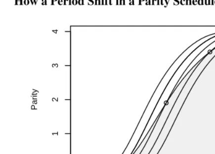
Figure 2 shows how a shift in a period schedule leads to a stretched cohort schedule. Here we plot the cumulative scheduleF0(a)in the example at 10 year intervals. We also
show in gray the parity schedule for the cohort starting reproductive life when the shift starts, and we mark the points where it “borrows” its cumulative fertility from the three central curves. Note that all schedules lead to a completed family size of four, but the cohort takes longer to climb that far.
To summarize, we have illustrated how a reduction in period fertility from 4.0 to 3.2 can result from delayed childbearing without changes in quantum. Noting that mean age of childbearing increases 0.2 years per year we obtain a TFR∗of 4.0. We can interpret this number as a counterfactual estimate of what the period TFR would have been if women had not delayed childbearing, in which case the mean age of childbearing would still be 29.2. We can also interpret it as the number of children that a synthetic cohort would have if the delay continued indefinitely, in which case mean age of childbearing would be 33.5. The last estimate pairs TFR∗withµ†, the estimate of mean age of childbearing
Figure 2: How a Period Shift in a Parity Schedule Translates into a Cohort Delay
20 30 40 50 60
0
1
2
3
4
Age
Parity
●
●
●
2.4 Cohort and period shifts
The foregoing results generalize to multiple cohorts if we assume that the cumulative period scheduleF(a, t)continues to shift according to Equation 7. For later cohorts this means not only that once childbearing starts it proceeds at a slower pace than before, but also that the start of childbearing itself is delayed. This implication of period-shift models will be of some significance when we turn to mortality, and represents a departure from accelerated failure time models.
Following exactly the same change of variables technique we used for the Zeng-Land cohort, we can show that the cohort born at timetfort≥ −a0has
TFRc(t) =TFR0 and µc(t) =µ†+rc(t+a0) (15)
wherercis the rate of change of cohort mean age of childbearing, and is related to the period derivative by
rc = r
1−r. (16)
Equation 16 is due to Zeng and Land (2002), who noted that period changes in tempo provide a distorted view of cohort changes in tempo. (They use the notationr∗ forr
c.)
Note that the cohort considered earlier was born att = −a0, and that evaluating these
expressions at that value leads to TFR†andµ†.
Figure 3: Shifting Period and Cohort Fertility Schedules
Time Age
ASFR
Period Shift
slope r
Time Age
ASFR
Cohort Shift
slope rc
but at slightly different ratesrandrc. Figure 3 illustrates this idea using model
Coale-Trussell schedules. The left panel shows a period schedule that is shifting to older ages at the rate ofr= 0.2years per year, and the right panel shows the corresponding cohort schedules shifting at the rate ofrc= 0.25years per cohort.
Thus, under a simple linear shift model cohort and period quantum are constant and differ by a factor1−rat time zero and later. Cohort and period tempo change over time. The period mean age of childbearing increases at the rate ofryears per year starting from
µ0at time zero. Cohort mean age of childbearing varies betweenµ0andµ†for the active
cohorts at time zero, and increases at the rate ofrcyears per cohort for cohorts that start
their reproductive careers after that. These results provide a way to translate cohort and period quantum and tempo, but the assumptions required are stronger than for a simple counterfactual interpretation of TFR∗.
3.
Mortality
Let us now turn our attention to mortality, focusing on a surface of age-period specific ratesµ(a, t)representing the force of mortality at ageaand timetfor the cohort born at
More often the mortality rates for fixedtare used to compute aperiodlife table, which may be interpreted in terms of a synthetic cohort that goes through life subject to the force of mortality prevailing at timet. Bongaarts and Feeney’s concern is that period measures, including the period expectation of life and the rates themselves, may be distorted by a tempo effect.
3.1 Mortality translation
Ryder (1964) noted that “the development of translation procedures has proven more difficult for mortality functions than for fertility functions” because of the multiplicative relationships involved in an attrition process, although he made some headway working with the logarithms of the rates. Keilman (1994) later obtained useful translation formulas for the hazards of non-repeatable events, but these do not lead to simple summary results such as Equation 4.
Further progress can be made working with asurvivalsurface whereS(a, t)represents the probability that someone born at timet−awill survive to ageaat timet,
S(a, t) = exp{− Z a
0
µ(x, t−a+x)dx}. (17)
A nice feature of this surface is that integrating along a diagonal leads to cohort life expectancy:
e(0c)(t) =
Z ∞
0
S(a, t+a)da. (18)
Unfortunately, integrating overafor fixedtdoesnotlead to period life expectancy unless mortality is constant. It does, however, lead to a meaningful alternative period measure of longevity, the cross-sectional average length of life (CAL) described by Guillot (2003):
CAL(t) =
Z ∞
0
S(a, t)da. (19)
The survival probabilitiesS(a, t)for fixed tmay be interpreted as the age distribution of a population that has a constant stream of births and is subject to the mortality risks
µ(a, t). Bongaarts and Feeney (2003) call this thestandardizedage distribution. CAL is a function of this age distribution and thus depends on past mortality, a point to which we will return later.
In addition to life expectancy and CAL it will be useful to defineα= R
aS(a)da/
R
the survival probabilities for the cohort now at its mean stationary age around the current age distribution using a first-order Taylor series, yields
e(0c)(t−α) = CAL(t) 1−rc
, (20)
whererc is the rate of change in the cohort mean stationary age. This shows that, to a first order of approximation, CAL falls below cohort life expectancy when mortality is declining, to an extent determined by the speed of the decline, provided we line up cohorts and periods using mean stationary age.
Guillot (2006) applies Ryder’s ideas using a somewhat different approach, but reaches essentially the same conclusions. He divides CAL(t)by an index of distributional distor-tion to obtain an adjusted measure, which can be interpreted as a weighted average of the life expectancies of all cohorts alive att. He then notes in an application to France that the result is close to the life expectancy of the cohort born at timet−A(t), whereA(t)is the mean age of the stationary population at timet, between 30 and 37 years for France in the twentieth century. Here we divide by1−rcinstead of the distortion index, and use
cohort rather than period mean age. But we both conclude that when mortality declines CAL falls below the life expectancy of the cohort near its mean stationary age. (I later show under different assumptions that CAL equals the life expectancy of the cohort now at its mean age at death.)
One could take this result to mean that CAL provides a distorted view of cohort life expectancy, or is subject to a tempo effect when mortality is declining, in much the same way that the period TFR distorts cohort fertility. I prefer to view it as indicating that when mortality is declining the age structure lags behind the cohort mortality schedule. In other words, it takes a while for a population to forget its past.
I realize that applying a formula developed for the quantum of fertility to the tempo of mortality seems unusual, if not plain wrong, but Ryder’s result is quite general. Given any age-period surface, it relates a cohort integral to a period integral and to the rate of change of the first cohort moment. In fertility we applied it to age-specific rates, so the integrals are measures of quantum and the first moment is tempo. In mortality we applied it to survival probabilities (or age distributions), so the integrals are mean survivals and the first moment is mean stationary age.
3.2 The Bongaarts-Feeney model
model in terms of a slowing down of the passage of time, just as we did for fertility. Later we discuss various period and cohort measures of longevity under the model.
LetS0(a)denote a survival function and letd0(a)andµ0(a)denote the corresponding
density and hazard functions. This could be a conventional period life table or a math-ematical model. We will assume that at time zero survival is governed byS0(a)in the
sense that all cohorts are following this schedule. This is equivalent to assuming that the population is stationary with age distributionS0(a).
Suppose, however, that at time zero all cohorts postpone death at the same rater. Consider specifically the cohort that has reached ageaat time zero, of which a fraction
S0(a)is still alive. We would expect a fractionS0(a+ 1)to be alive a year later at age
a+ 1, but instead we observe that the proportion surviving has increased toS0(a+ 1−r).
It is precisely as if the cohort had aged only1−ryears in one year. This type of model is known in the statistical literature as an accelerated life model, see for example Kalbfleisch and Prentice (2002). The situation is similar to taking a pill that prevents death (and stops aging) for a fractionrof the year, but I prefer to view the process as developing in continuous time.
Remarkably, this model is equivalent for all active cohorts to a period shift in the standardized age distribution, where
S(a, t) =
1 ifa < rt S0(a−rt) ifa≥rt
(21)
For example the survival probabilities for the cohort considered in the previous paragraph areS(a,0) =S0(a)andS(a+ 1,1) =S0(a+ 1−r). If we compute a cohort derivative,
differentiating Equation 21 with respect to both age and time, and changing sign, we obtain a density reflecting the age distribution of deaths at each time
d(a, t) =
0 ifa < rt
d0(a−rt)(1−r) ifa≥rt.
(22)
Note thatd(a, t)is a probability density function only for a cohort, i.e. if we consider
d(a, c+a)for fixedc. The period profile is not a real density but a collection of den-sities for various cohorts, and in this model it integrates to1−r, not one. Bongaarts and Feeney (2003) call the integral ofd(a, t)for fixedtthe total mortality rate (TMR). Watcher (2005) notes that it can be interpreted as a period count of deaths.
If we divide the deaths d(a, t)by the numbers exposedS(a, t)we obtain the age-period specific force of mortality
µ(a, t) =
0 ifa < rt
µ0(a−rt)(1−r) ifa≥rt.
This is both a period and a cohort hazard, pertaining to timetand to the cohort born at
t−a. Note that when all cohorts start delaying death at the same rate the hazard is instantly deflated by a factor1−rand starts shifting to older ages. This is clearly a tempo effect, as it is caused by a delay in death. I don’t believe, however, that it is a distortion. The only way that cohorts can delay death is by dying at lower rates, so I view the reduction in hazards as real. The interesting question concerns the implications of this change for longevity.
It will be useful to introduce for completeness two additional functions defined by Bongaarts and Feeney (2003) in (their) Equations 5a and 5b. If we differentiateS(a, t)
with respect to time only (as opposed to time and age simultaneously) we obtain the death density
ds(a, t) =d0(a−rt), (24)
and dividing this by the survivorsS(a, t)we obtain the hazard
µs(a, t) =µ0(a−rt). (25)
These are proper density and hazard functions fora ≥ rtand can best be viewed as inherent features of the standardized age distributionS(a, t), so I will call then the age-distribution density and hazard, respectively. Note that under the period shift model the observed force of mortalityµ(a, t)is proportional to the age distribution hazardµs(a, t), with proportionality factor1−r. This is called theproportionalityassumption in the Bongaarts-Feeney framework.
I should also note that Bongaarts and Feeney consider a more general shift model where the rate of delay is not a constantrbut a function of timer(t). I stick to the linear case because it is simpler and leads to explicit results for cohorts.
3.3 Four measures of longevity
Bongaarts and Feeney (2003) consider four measures of longevity, denotedM1toM4.
Three of them are equal under the period-shift model of the previous section. The odd one out is period life expectancy.
The first measure is cohort average length of life (CAL)
M1(t) =CAL(t) =
Z ∞
0
S(a, t)da. (26)
This measure is easily computed by integrating the standardized age distribution. From Equation 21 we find that under the period shift model
where CAL(0)is both CAL and the conventional expectation of life in the baseline sched-uleS0(a). CAL may be computed as an ordinary mean age at death where deaths are
obtained by applying the age-distribution hazardµs(a, t)to the standardized age distri-butionS(a, t). Interestingly, CAL doesn’t change when cohorts start postponing death, but it starts increasing at the rate ofryears per year as long as the shift (or slow down of time) continues. This occurs because CAL is based solely on the age structure at timet, and does not respond to changes in mortality until these are reflected in the age structure.
The second measure is standardized mean age at death
M2(t) =
Z ∞
0
ad(a, t)da/
Z ∞
0
d(a, t)da, (28)
which is based on the standardized age distribution of deaths at timet. The deaths in this index result from applying the current force of mortalityµ(a, t)to the standardized age distributionS(a, t), and may thus be viewed as a measure that depends both on current mortality risks and the current age distribution.
Under the period-shift model the force of mortalityµ(a, t)and the age-distribution hazardµs(a, t)are proportional, with proportionality factor1−r. Because this factor
appears both in the numerator and denominator of the mean it cancels out, soM2(t) =
M1(t)as noted by Bongaarts and Feeney (2003). If the proportionality assumption is not
satisfied, however, the two indices will differ.
The third measure is conventional period life expectancy
M3(t) =e (p) 0 (t) =
Z ∞
0
exp{− Z a
0
µ(x, t)dx}da. (29)
This index may also be viewed as an ordinary mean age at death where deaths result from applying the force of mortalityµ(a, t)to the stationary population implied by that hazard, which is of course the period survival functionexp{−Ra
0 µ(x, t)da}(not to be confused
withS(a, t)). This measure depends on the current force of mortality only.
Under the period shift model the force of mortalityµ(a, t)is proportional toµs(a, t)
and therefore the period survival function is a power of the standardized age structure, but there is no simple relationship betweenM3(t)and eitherM1(t)orM2(t).
Note that when cohorts start postponing death the conventional expectation of life reacts instantly. Because it depends only on the force of mortalityµ(a, t), which has been deflated by a factor1−r, conventional life expectancye0 will increase. This is
again a tempo effect, but in my view is not a distortion. Conventional life expectancy is just a summary of age-period specific mortality, and responds appropriately by increasing when the rates decline. In particular, the synthetic cohort interpretation ofe0as the mean
The fourth measure is the Bongaarts-Feeney tempo-adjusted life expectancy. This index seeks to remove the tempo effect from the force of mortality dividing by1−rand is therefore defined as
M4(t) =
Z ∞
0
exp{− Z a
0
µ(x, t)/(1−r)dx}da. (30)
Under the period-shift modelµ(a, t)is proportional toµs(a, t)with proportionality factor (1−r)and thereforeM4(t) =M1(t) =M2(t), as noted by Bongaarts and Feeney (2003).
In this case the adjusted measure can be viewed as an ingenious way to estimate CAL or mean age at death from the observed hazard. If the model does not hold, however,M4(t)
is a different measure that ostensibly depends only on the current force of mortality and the rate of delayr, but in practice requires knowledge of the standardized age distribution for estimation. Watcher (2005) provides a characterization of M4(t)that clarifies this
issue.
To summarize, when cohorts start delaying death conventional life expectancy re-acts instantly, whereas the other three measures react more slowly, increasing only as the changes work their way into the age structure. The fundamental issue is whether this is a bias or distortion in conventional life expectancy. I argue that it is just a reflection of the fact that when mortality declines the age structure lags behind the force of mortality. To further explore this issue we now look at the cohort implications of the period-shift model.
3.4 Cohort survival
Consider again the cohort born at the time the period shift, or the slowing down of the passage of time, starts. This cohort would have been expected to follow the schedule
S0(a)but instead will follow a stretched schedule, where the probability of surviving to
ageais
S†(a) =S0(a(1−r)). (31)
This result follows directly from the period-shift model in Equation 21 and shows that each calendar year the cohort ages only1−ryears.
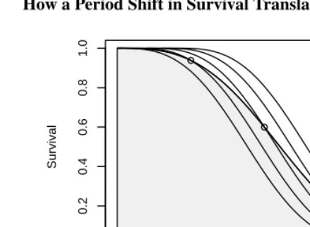
Figure 4: How a Period Shift in Survival Translates into a Cohort Delay
0 20 40 60 80 100
0.0
0.2
0.4
0.6
0.8
1.0
Age
Survival
●
●
●
We can compute the expectation of life underS†(a)using the same change of vari-ables technique that we used in the case of fertility:
e†0=
Z ∞
0
S0(a(1−r))da=
Z ∞
0
S0(y)
dy 1−r =
e0
1−r. (32)
We find that ifr > 0the expectation of life under a shifting schedule exceeds the value it would have if the schedule remained fixed. The area under the original curve ise0, the
shaded area under the stretched curve ise†0.
Note by way of illustration that life expectancy in the U.S. today is 77.3 under a fixed mortality schedule, but would be 85.8 if the schedule shifted 0.1 years per year, which is the observed gain in period life expectancy between 2001 and 2002. The value 85.8 is computed simply as 77.3/0.9.
Let us return toS†(a), the survival function that applies to our synthetic cohort. Dif-ferentiating we find the density to be
d†(a) = d daS
†(a) = d
daS0(a(1−r)) =d0(a(1−r))(1−r). (33)
The hazard, computed as the ratio of deaths to survival, is
µ†(a) =d†(a)/S†(a) =µ0(a(1−r))(1−r). (34)
are consistent with Equations 22 and 23 in the previous section, and thus with equations 8b and 8c in Bongaarts and Feeney (2003). (We showed before that their dtdM2(t) =r.)
We note again that as soon as time slows down the hazard is deflated by a factor
1−r, which is how the cohort manages to live longer. Consider an example where the baseline survivalS0(a)is Weibull with parameterspandλ, soS0(a) = exp{−(λa)p}.
In this case the stretched survival S†(a)is also Weibull with parameters pandλ† = λ(1−r), so the shift and consequent slowing down of the passage of time translate into a proportionate reduction in the hazard at all ages. Kalbfleisch and Prentice (2002) show that the Weibull is the only distribution where the accelerated life and proportional hazards families coincide.
For an example more relevant to human mortality, at least in adult ages, consider a Gompertz model with parametersαandβ, where the baseline hazardµ0(a) = exp{α+
βa}increases exponentially with age. In this case the stretched survival is also Gompertz but with parametersα†=α+ log(1−r)andβ†=β(1−r), a result that follows directly from the general expression given above. In this case the change in the hazard is not proportional, but relatively larger at older ages. For a country such as the U.S., where adult mortality is roughly Gompertz, a shift of 0.1 years per year starting at age 30 would reduce the hazard by 10% at age 30, 30% at age 60 and 46% at age 90. As a result a 30 year old, who is expected to live another 48.4 years under current conditions, would live on average about 53.8. (These calculations are based onα=−9.696andβ = 0.0855, which impliesα† =−9.545andβ† = 0.07694. Note that for a shift starting at agea0
rather than zeroα†=α+ log(1−r) +βra0. The value ofe†0= 53.8can be obtained as
48.4/0.9 or by numerical integration of the Gompertz hazard.)
These results can be extended to multiple cohorts, just as we did in the case of fertility, by assuming that the standardized age distribution continues to shift at a constant rate. Using essentially the same argument as in the previous section, we can show that the cohort born at timet >0goes through the survival schedule
S(a, t+a) =
1 ifa < tr/(1−r)
S0(a−r(t+a)) otherwise
(35)
and thus has life expectancy
e(0c)(t) =e†0+rct, (36)
wheree†0is the life expectancy of the cohort born at time zero andrc, the rate of change in cohort life expectancy, is
rc= r
1−r. (37)
The cohort born at time zero experiences just a stretching of the survival functionS0(a),
experience no mortality until they reach agerct, at which time they join a stretched and shifted schedule. This feature makes the model less realistic in multiple-cohort settings unless one restricts its applicability, as Bongaarts and Feeney do, to the adult ages, say above 30, in low mortality populations.
With these caveats, the foregoing results allow us to relate period CAL or mean age at death to cohort life expectancy. As we noted in the previous section, when mortality declines the age structure lags behind the force of mortality and as a result
CAL(t)< e(0p)(t)< e(0c)(t). (38)
Under the period-shift model we can be a bit more precise. We can show that the Bongaarts-Feeney measureM4, which is then the same as CAL,M1andM2, is the life expectancy
of the cohort now at its mean age at death:
CAL(t+e(0c)(t)) =e(0c)(t), (39)
a result easily verified by direct substitution, noting that the cohort born atthas mean age at death(e0+rt)/(1−r). Alternatively, one can go back in time and note that the cohort
dying today was born at time(t−e†0)/(1 +rc)and has life expectancy CAL(t).
Goldstein (2006) has also derived the translation formula (39) and has used it to show that under a continuing linear shift the cohort born today would have life expectancy given by equation (32); this provides increased confidence in these results.
To summarize, conventional life expectancye0measures how long a new born would
live under current rates. This may not be a realistic estimate if mortality is declining. Under a period-shift model we have shown that a new born would in fact live longer,
e†0years. On the other hand period CAL, mean age at death and the Bongaarts-Feeney adjusted measureM4would all be lower, corresponding to the mean age at death of the
cohort now reaching its life expectancy, provided the assumptions underlying the simpler linear shift model are satisfied.
3.5 A proportional hazards model
We now consider an example where the assumption is not quite satisfied, and therefore CAL,M2andM4 differ. Specifically, consider a population with a constant stream of
births and no mortality before age 30. Suppose the force of mortality follows a Gompertz function withα=−9.997andβ = 0.0855, which as noted earlier fits very closely the U.S. 2002 life table. Suppose further that mortality has been constant long enough for the population to become stationary. In this case all four measures, CAL, mean age at death,
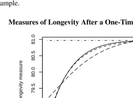
Suppose now that at time zero the force of mortality declines 20% at all ages. The con-ventional period life expectancy, being just a summary of age-specific mortality, would increase instantly to 80.97 to reflect this improvement. One has to be careful no to con-clude that all cohorts will live this long, as the calculation applies only to the cohort age 30 at time zero, assuming mortality remains constant thereafter. CAL, on the other hand, doesn’t change at time zero but starts increasing immediately afterwards as the decline in mortality is reflected on the standardized age distribution. Eventually the population becomes stationary again and CAL reaches 80.97. Figure 5 shows the trajectory of CAL for this example.
Figure 5: Measures of Longevity After a One-Time Reduction in Hazard
0 10 20 30 40 50 60 70
78.5
79.0
79.5
80.0
80.5
81.0
Time since decline
Longevity measure
M_1
M_2
M_3
M_4
Cohort
Mean age at death doesn’t change instantly either. Although this index depends on the observed force of mortality, which is 20% lower at time zero, the reduction factor appears both in the numerator and denominator and cancels out. It is only as the reduction works its way into the age structure that mean age at death starts to increase, eventually reaching 80.97. Figure 5 shows that the trajectory of mean age at death is very similar to CAL. The Bongaarts-Feeney tempo-adjusted measure depends on the force of mortality and a correction factor based onr, which I estimated using the TMR. (Using a numerical derivative of M2(t)gives very similar results except for the first two years.) The key
result is thatM4is very similar to the other two measures. It takes them nearly sixty years
to fully reflect the instantaneous change in mortality that occurred at time zero.
expectancy on the year when it reaches its mean age at death. We note that the three mea-sures of longevity track the increase in cohort life expectancy, albeit only approximately.
4.
Discussion
This paper has emphasized similarities between the analysis of fertility and mortality. I have argued that Ryder’s translation formula can be applied quite generally to demo-graphic surfaces. When the surface represents age-specific fertility rates the formula translates period and cohort quantum. When the surface represents survival probabilities the formula translates period and cohort tempo, but using CAL rather than conventional life expectancy. The common theme is that period and cohort demographic summaries can differ in times of change. I believe that labelling these differences a bias or distor-tion has been unfortunate. Period aggregates provide convenient summaries, while cohort aggregates are often needed to fully understand the underlying process.
I have also stressed the fact that the Bongaarts-Feeney framework is essentially the same for fertility and mortality, postulating a period shift in a cumulative schedule repre-senting average parity or survival probabilities. The shift can be motivated by assuming that all cohorts delay childbearing or postpone death at the same rate, and is closely linked to accelerated failure time models used in survival analysis. The shift results in a propor-tionate reduction in fertility or mortality rates, which also move to older ages. The model applies to multiple cohorts but requires assuming that later cohorts experience not just a slowing down of time but also a delay in the onset of exposure, an assumption that may be less realistic and, in the case of mortality, requires restricting application to adult ages in low mortality populations. I have also proposed measures of tempo under changing fertil-ity or mortalfertil-ity which complement the Zeng-Land interpretation of the Bongaarts-Feeney adjustment by applying to the same synthetic cohort.
There are two reasons why mortality is different, even if the same period-shift model applies. First, mortality is a pure tempo phenomenon; everyone dies exactly one time and the only question is when. Consequently, a reduction in the period force of mortality can only mean that cohorts are delaying death. There is no risk of misinterpretation, and therefore, one might argue, no need for adjustment. Bongaarts and Feeney implicitly acknowledge this point when they note that mean age at death, which they view as a direct analog of mean age of childbearing, needs no adjustment. They do adjust the force of mortality, of course, but I view this adjustment as merely a device to bring the conventional calculation of life expectancy inline with CAL or mean age at death. I see no bias or distortion in the observed force of mortality, just as I see no bias in age-specific fertility, and the best proof of that is the fact that cohort survival is determined entirely by
µ(a, t), not by its tempo-adjusted version. The question then is whether we should use standardized mean age at death or conventional life expectancy as a measure of longevity. That brings us directly to the second reason why mortality is different, and it has to do with exposure. In fertility all women are exposed to have a birth, whether they have had one before or not, which makesf(a, t)a true event-exposure rate. Both the cohort and period TFR and mean age of childbearing are summaries of these rates and are not affected by exposure. In the case of mortality only survivors are at risk of dying, which is why analytical interest usually focuses on the force of mortalityµ(a, t), which acts on survivorsS(a, t) to produce deaths d(a, t). For a cohort the choice of measure is immaterial because exposure is itself determined by the force of mortality and as a result conventional life expectancy and mean age at death are identical. For a period the two measures can be quite different when mortality is changing. Conventional life expectancy depends only on the period force of mortalityµ(a, t), whereas mean age at death depends also on S(a, t) and thus on the population’s past mortality history. We have seen that under the strong assumption of a linear-shift model, mean age at death coincides with the life expectancy of the cohort now reaching its mean age at death.
The question we asked at the outset, ‘How long do we live?’, can thus be seen to have different answers depending on our precise definition of ‘we’. Conventional life expectancy applies to a hypothetical cohort that is exposed to a constant set of rates. It has the great merit of also applying to everyone else when mortality is constant. But when mortality is changing the construction is less useful; why ask how long someone would live subject to these rates if they are changing? We know that they would probably live longer than that, and we can estimate how much longer if we are willing to make strong assumptions about future changes. In particular, a continuing linear shift to older ages leads toe†0, the simple measure of life expectancy under changing mortality proposed here. It is also the case that when mortality is declining no cohort has yet lived that long, or even as long ase0would imply. The Bongaarts-Feeney measure tells us how long those
holds. The fact that those dying today haven’t lived as long as today’s newborns will probably live, under either fixed or changing rates, is not a bias or distortion; it’s just a fact of life.
The foregoing discussion has emphasized the practical interpretation of various mea-sures of longevity while implicitly accepting the conventional view that mortality change is driven by the hazard function. But the Bongaarts-Feeney approach is fundamentally different; it views mortality change as driven by gains in longevity that shift the age distribution. This deflates the hazard by a factor1−rand shifts it to older ages. Un-fortunately, it is difficult to differentiate these frameworks empirically because the age patterns in low-mortality countries are very close to a Gompertz model, where a propor-tionate reduction in the hazard cannot be distinguished from a shift to older ages. But if mortality were to stop declining we would soon know, because the period-shift model predicts an increase in the hazard as the factor1−rdisappears and our past catches up with us, whereas the conventional view is that the hazard would stay constant. Faced with such choice, one may very well prefer to see hazards continue to decline and live longer with the uncertainty.
5. Acknowledgments
References
Arias, E. (2004). United States life tables, 2002. National Vital Statistics Reports, 53(6):271–291.
Bongaarts, J. and Feeney, G. (1998). On the quantum and tempo of fertility. Population and Development Review, 24(2):271–291.
Bongaarts, J. and Feeney, G. (2000). On the quantum and tempo of fertility: Reply. Population and Development Review, 26(3):560–564.
Bongaarts, J. and Feeney, G. (2002). How long do we live? Population and Development Review, 28(1):13–29.
Bongaarts, J. and Feeney, G. (2003). Estimating mean lifetime. Proceedings of the Na-tional Academy of Sciences, 100(23):13127–13133.
Bongaarts, J. and Feeney, G. (2005). The quantum and tempo of life-cycle events. Pol-icy Research Division Working Paper, New York City: Population Council, 207. http://www.popcouncil.org/.
Coale, A. J. (1971). Age patterns of marriage.Population Studies, 25(2):193–214.
Coale, A. J. and Trussell, T. J. (1974). Model fertility schedules: Variations in the age structure of childbearing in human populations.Population Index, 40:185–258.
Goldstein, J. R. (2006). Found in translation? A cohort perspective on tempo-adjusted life expectancy. Demographic Research, 14(5):71–84. http://www.demographic-research.org/volumes/vol14/5/.
Guillot, M. (2003). The cross-sectional average length of life (CAL): A cross-sectional mortality measure that reflects the experience of cohorts. Population Studies, 57(1):41–54.
Guillot, M. (2006). Tempo effects in mortality: An appraisal. Demographic Research, 14(1):1–26. http://www.demographic-research.org/volumes/vol14/1/.
Kalbfleisch, J. D. and Prentice, R. L. (2002). The Statistical Analysis of Failure Time Data. John Wiley and Sons, New York, 2nd edition.
48(2):341–357.
N´ı Bhrolch´ain, M. (1992). Period paramount? a critique of the cohort approach to fertility. Population and Development Review, 18:599–629.
Ryder, N. B. (1964). The process of demographic translation.Demography, 1(1):74–82.
Schoen, R. (2004). Timing effects and the interpretation of period fertility.Demography, 41(4):801–819.
van Imhoff, E. and Keilman, N. (2000). On the quantum and tempo of fertility: Comment. Population and Development Review, 26:549–553.
Vaupel, J. W. (2002). Life expectancy at current rates vs. current conditions: A reflex-ion stimulated by Bongaarts and Feeney’s “How long do we live?”. Demographic Research, 7. Article 8.
Wachter, K. W. (2005). Tempo and its Tribulations.Demographic Research, 13(9):201– 222. http://www.demographic-research.org/volumes/vol13/9/.
Zeng Yi and Land, K. C. (2001). A sensitivity analysis of the Bongaarts-Feeney method for adjusting bias in observed period total fertility rates.Demography, 38:17–28.