A structure-exploiting numbering algorithm for ﬁnite elements on extruded meshes, and its performance evaluation in Firedrake

(1)

Geosci. Model Dev., 9, 3803–3815, 2016 www.geosci-model-dev.net/9/3803/2016/ doi:10.5194/gmd-9-3803-2016

A structure-exploiting numbering algorithm for finite elements on

extruded meshes, and its performance evaluation in Firedrake

Gheorghe-Teodor Bercea1_{, Andrew T. T. McRae}2,3,4_{, David A. Ham}3_{, Lawrence Mitchell}1,3_{, Florian Rathgeber}1,5_, Luigi Nardi1_{, Fabio Luporini}1_{, and Paul H. J. Kelly}1

1_{Department of Computing, Imperial College London, London, SW7 2AZ, UK} 2_{The Grantham Institute, Imperial College London, London, SW7 2AZ, UK} 3_{Department of Mathematics, Imperial College London, London, SW7 2AZ, UK} 4_{Department of Mathematical Sciences, University of Bath, Bath, BA2 7AY, UK}

5_{European Centre for Medium-Range Weather Forecasts (ECMWF), Reading, RG2 9AX, UK}

Correspondence to:Gheorghe-Teodor Bercea ([email protected])

Received: 27 May 2016 – Published in Geosci. Model Dev. Discuss.: 9 June 2016

Revised: 16 September 2016 – Accepted: 26 September 2016 – Published: 27 October 2016

Abstract.We present a generic algorithm for numbering and then efficiently iterating over the data values attached to an extruded mesh. An extruded mesh is formed by replicating an existing mesh, assumed to be unstructured, to form layers of prismatic cells. Applications of extruded meshes include, but are not limited to, the representation of three-dimensional high aspect ratio domains employed by geophysical finite el-ement simulations. These meshes are structured in the ex-truded direction. The algorithm presented here exploits this structure to avoid the performance penalty traditionally asso-ciated with unstructured meshes. We evaluate the implemen-tation of this algorithm in the Firedrake finite element sys-tem on a range of low compute intensity operations which constitute worst cases for data layout performance explo-ration. The experiments show that having structure along the extruded direction enables the cost of the indirect data ac-cesses to be amortized after 10–20 layers as long as the un-derlying mesh is well ordered. We characterize the result-ing spatial and temporal reuse in a representative set of both continuous-Galerkin and discontinuous-Galerkin discretiza-tions. On meshes with realistic numbers of layers the per-formance achieved is between 70 and 90 % of a theoretical hardware-specific limit.

1 Introduction

In the field of numerical simulation of fluids and structures, there is traditionally considered to be a tension between the computational efficiency and ease of implementation of structured grid models, and the flexible geometry and resolu-tion offered by unstructured meshes.

In particular, one of the grand challenges in simulation science is modelling the ocean and atmosphere for the pur-poses of predicting the weather or understanding the Earth’s climate system. The current generation of large-scale opera-tional atmosphere and ocean models almost all employ struc-tured meshes (Slingo et al., 2009). However, requirements for geometric flexibility as well as the need to overcome scal-ability issues created by the poles of structured meshes have led in recent years to a number of national projects to cre-ate unstructured mesh models (Ford et al., 2013; Zängl et al., 2015; Skamarock et al., 2012).

(2)

meshes employed in the new generation of models are the result of extruding an unstructured two-dimensional mesh to form a layered mesh of prismatic elements.

This layered structure was exploited in Macdonald et al. (2011) to create a numbering for a finite volume atmospheric model such that iteration from one cell to the next within a vertical column required only direct addressing. They show that when only paying the price of indirect addressing on the base mesh there is less than 5 % performance difference be-tween two implementations of an atmospheric model which treat the same icosahedral mesh first as fully structured and then as partially structured (extruded). One of the caveats of that comparison is that the underlying mesh is fully struc-tured in both cases, which presents an advantage to the indi-rect addressing scheme which is not present for more general unstructured meshes.

Exploiting the anisotropic nature of domains has seen var-ious software developments in varvar-ious fields. For example, p6est(Isaac et al., 2015 and Isaac, 2015, Sect. 2.3), a pack-age for 2+1 dimensional adaptive mesh refinement, was de-veloped to maintain columnwise numbering for numerical reasons in ice sheet modelling, but does not support gen-eral unstructured base meshes. The DUNE-PrismGrid mod-ule (Gersbacher, 2012) provides extruded meshes for any base DUNE grid, but does not describe a degree of freedom numbering or provide detailed performance characteristics of the iteration on extruded meshes. The Model for Predic-tion Across Scales (MPAS) uses a column innermost num-bering for their C-grid atmospheric and ocean model (Sarje et al., 2015). Their implementation is limited to the single discretization employed by that model.

A key motivation for this work was to provide an efficient mechanism for the implementation of the layered finite el-ement numerics which have been adopted by the UK Met Office’s Gung Ho programme to develop a new atmospheric dynamical core. The algorithms here have been adopted by the Met Office for this purpose (Ford et al., 2013). While geo-physical applications motivate this work, the algorithms and their implementation in Firedrake (Rathgeber et al., 2016) are more general and could be applied to any high aspect ra-tio domain.

Contributions

– We generalize the numbering algorithm in Macdonald et al. (2011) to the full range of finite element discretiza-tions.

– We demonstrate the effectiveness of the algorithm with respect to absolute hardware performance limits.

2 Unstructured meshes

In this section we briefly restate the data model for un-structured meshes introduced in Logg (2009) and Knepley

and Karpeev (2009). In Sect. 2.2 we rigorously define a

mesh, and explain mesh topology, geometry, and

number-ing. In Sect. 2.3 we explain how data may be associated with meshes.

2.1 Terminology

When describing a mesh, we need some way of specifying the neighbours of a given entity. This is always possible

us-ingindirect addressingin which the neighbours are explicitly

enumerated, and sometimes possible withdirect addressing

where a closed-form mathematical expression suffices. In what follows we start with abase meshwhich we will

extrudeto form a mesh of higher topological dimension. Due

to geophysical considerations, we refer to the plane of the base mesh as thehorizontaland to the layers as thevertical.

We will also employ the definition of agraphas a setV and a setEof edges where each edge represents the relation-ships between the elements of the setV.

2.2 Meshes

A mesh is a decomposition of a simulation domain into non-overlapping polygonal or polyhedral cells. We consider meshes used in algorithms for the automatic numerical so-lution of partial differential equations. These meshes bine topology and geometry. The topology of a mesh is com-posed of mesh entities (such as vertices, edges, and cells) and the adjacency relationships between them (cells to vertices or edges to cells). The geometry of the mesh is represented by coordinates which define the position of the mesh entities in space.

Every mesh entity has a topological dimension given by the minimum number of spatial dimensions required to rep-resent that entity. We defineDto be the minimum number of spatial dimensions needed to represent a mesh and all its entities. A vertex is representable in zero-dimensional space; similarly, an edge is a one-dimensional entity and a cell aD -dimensional entity. In a two--dimensional mesh of triangles, for example, the entities are the vertices, edges, and triangle cells with topological dimensions 0, 1, and 2 respectively. The minimum number of geometric dimensions needed to represent the mesh and all its entities isD=2.

A mesh can be represented by several graphs. Each graph consists of a multi-type setV and a typed adjacency relation-ship Adjd1,d2 betweend1 andd2 typed elements inV. The

type of an entity inV is simply its dimension. The adjacency graphs will always map from a set of uniform dimension to a set of uniform dimension. Attaching types to elements ofV enables graphs to capture the relationships between different mesh entities, for example cells and vertices, and edges and vertices.

We writeVdto mean the set of mesh entities of topological dimensiondwhere 0≤d≤D:

(3)

G.-T. Bercea et al.: A numbering algorithm for finite elements on extruded meshes 3805

whereNd is the number of entities of dimensiond. The set V is then simply the union of theVds:

V = [

0≤d≤D

Vd. (2)

Every mesh entity has a number of adjacent entities. The mesh–element connectivity relationships are used to specify the way mesh entities are connected. For a given mesh of topological dimension Dthere are(D+1)2different types of adjacency relationships. To define the mesh, only a mini-mal subset of relationships from which all the others can be derived is required. For example, as shown in Logg (2009), the complete set of adjacency relationships may be derived from the cell–vertex adjacency.

We write

Adjd1,d2(v)=(v1, v2, . . ., vk) (3)

to specify the entitiesv1, v2, . . ., vk∈Vd₂adjacent tov∈Vd₁. In a mesh with a very regular topology, there may be a closed-form mathematical expression for the adjacency re-lationship Adjd1,d2(v). Such meshes are termedstructured.

However, since we are also interested in supporting more general unstructured meshes, we must store the lists of

ad-jacent entities explicitly. 2.3 Attaching data to meshes

Every mesh entity has a number of values associated with it. These values are also known as degrees of freedomand

they are the discrete representation of the continuous data fields of the domain. As the degrees of freedom are uniquely associated with mesh entities, the mesh topology can be used to access the degrees of freedom local to any entity using the connectivity relationships.

Afinite element discretizationassociates a number of

de-grees of freedom with each entity of the mesh. A function

space uses the discretization to define a numbering for all

the degrees of freedom. Multiple different function spaces may be defined on a mesh and each function space may have several data fields associated with it. In the case of a trian-gular mesh for example, a piecewise linear function space will associate a degree of freedom with every vertex of the mesh, while a cubic function space will associate one degree of freedom with every vertex, two degrees of freedom with every edge, and one degree of freedom with every cell. In the former case there will be 3 degrees of freedom adjacent to a cell, and a total of 10 in the latter case.

The data associated with the mesh also need to be num-bered. The choice of numbering can have a significant effect on the computational efficiency of calculations over the mesh (Günther et al., 2006; Lange et al., 2016; Yoon et al., 2005). 2.4 Kernels and stencils

The most common operation performed on meshes is the lo-cal application of a function or kernel while traversing or

iteratingover a homogeneous subset of mesh entities. The

kernel is executed once for each such mesh entity and acts on the degrees of freedom in a stencil composed of the

mesh entities adjacent to the the iterated entity. For exam-ple, a finite element operator evaluating an integral over the domain would iterate over the mesh cells and access data through a stencil comprising the degrees of freedom on that cell and its adjacent facets, edges, and vertices. For a more in-depth discussion on the construction of stencils on un-structured meshes, the reader is referred to Logg (2009) and Knepley and Karpeev (2009). In theory, this requires cell-to-facets, cell-to-edges, and cell-to-vertices adjacency relation-ships (cell-to-cell is implicit). In practice the three different relationships may be composed into a single adjacency re-lationship which references the data associated with all the different adjacent entity types.

In the unstructured case, we store an explicit list (also known as a map) L(e) for each type of stencil operation which given a topological entityereturns the set of degrees of freedom in the stencil at that entity.

3 Extruded meshes

In Sect. 3.1 we introduce extruded meshes and in Sect. 3.2 we show how the entities and the data are to be numbered. In Sect. 3.3 we present the extruded mesh iteration algorithm and the offset computation for the direct addressing scheme along the vertical direction.

3.1 Definition of an extruded mesh

An extruded mesh consists of a base mesh which is repli-cated a fixed number of times in a layered structure1_{. A mesh} of topological dimensionD becomes an extruded mesh of topological dimensionD+1.

The mesh definition can be extended to include extruded meshes. Let mesh M=(V ,Adj) be a non-extruded mesh where Adj stands for all the valid adjacency relationships of M. An extruded mesh which hasMas the base mesh can be defined as a triple(Vextr,Adjextr, λ)where Adjextr is the set of valid adjacency relationships andλ∈N+ is the number

of intervals over which the mesh is extruded. This implies that there areλ+1 vertices in the extruded direction. Before we can defineVextr and Adjextr several concepts have to be introduced.

3.1.1 Tensor product cells

The effect of the extrusion process on the base mesh can al-ways be captured by associating a line segment with the ver-tical direction. We writeD_bfor the topological dimension of 1_{For ease of exposition, we discuss the case where each mesh}

(4)

Figure 1.Extruded mesh entities belonging to the base mesh to be extruded (left to right): vertices, horizontal edges, horizontal facets.

Figure 2. Mesh entities used in the extrusion process to connect entities in Fig. 1 (left to right): vertical edges, vertical facets, three-dimensional cells.

the base mesh, while the topological dimension of the verti-cal mesh is always equal to 1.

As a consequence, the cells of the extruded mesh are prisms formed by taking the tensor product of the base mesh cell with the vertical line segment. For example, each trian-gle becomes a triangular prism. The construction of tensor product cells and finite element spaces on them is considered in more detail in McRae et al. (2016).

3.1.2 Extruded mesh entities

The extrusion process introduces new types of mesh entities reflecting the connectivity between layers. The pairs of cor-responding entities of dimensiondin adjacent layers are con-nected using entities of dimensiond+1. In a triangular mesh for example (Fig. 1), the corresponding vertices are con-nected using vertical edges, edges contained in each layer are connected by quadrilateral facets, and the two-dimensional triangle faces are connected by a three-dimensional triangu-lar prism (Fig. 2).

The topological dimension on its own is no longer enough to distinguish between the different types of entities and their orientation. Instead entities are characterized by a pair com-posed of the horizontal and vertical dimensions. In the case of a two-dimensional triangular base mesh, the set of dimen-sions is{0,1,2}. The line segment of the vertical can be de-scribed by the set of dimensions{0,1}. The Cartesian product of the two sets yields a set of pairs (Eq. 4) which can be used to uniquely identify mesh entities.

{(0,0), (0,1), (1,0), (1,1), (2,0), (2,1)} (4) We refer to the components of each pair as the horizontal

and verticaldimensions of the entity respectively. Table 1

shows the mapping between the mesh entity types and their descriptor.

3.1.3 Extruded mesh entity numbering

We writeVd1,d2to denote the set of topological entities which

are the tensor product of entities of dimensionsd₁in the

hor-Table 1.Topological dimensions of extruded mesh entities.D_b

de-notes the topological dimension of the base mesh.

Mesh entity Dimensions

Vertex (0,0)

Vertical edge (0,1)

Horizontal edge (1,0)

Vertical facet (D_b−1,1)

Horizontal facet (D_b,0)

Cell (D_b,1)

izontal andd₂in the vertical (0≤d₁≤D_band 0≤d₂≤1): Vd1,d2=

((d₁, d₂), (i, l))|0≤i≤Nd1

−1,0≤l≤λ−d2}, (5)

whereNd₁ is the number of entities of dimensiond1in the base mesh andλis the number of edges in the extruded di-rection. The subtraction ofd₂fromλaccounts for the fence-post error caused by the fact that there is always one fewer edge than vertex in the vertical direction.

The complete set of extruded mesh entities is then Vextr= [

0≤d1≤Db 0≤d2≤1

Vd1,d2. (6)

These entities are those drawn for the case of an extruded triangle in Fig. 3.

Similarly we must extend the indexing of the adjacency relationships, writing

Adjextr_(d₁_,d₂_),(d₃_,d₄₎(v)=(v₁, v₂, . . ., vk), (7) wherev∈Vd1,d2 andv1, v2, . . ., vk∈Vd3,d4.

3.2 Attaching data to extruded meshes

Identically to the case of non-extruded meshes, function spaces over an extruded mesh associate degrees of freedom with the (extended) set of mesh entities. A constant num-ber of degrees of freedom is associated with each entity of a given type.

(5)

G.-T. Bercea et al.: A numbering algorithm for finite elements on extruded meshes 3807 G.-T. Bercea et al.: A numbering algorithm for finite elements on extruded meshes which avoids the unstructured mesh penalty5

Algorithm 1Computing the global numbering for degrees of freedom on an extruded mesh

Require: V: the set of base mesh entities

Require: λ: the number of vertical intervals

Require: δ((d₁, d₂)): the number of DoFs associated with each

(d₁, d₂)entity

Ensure: dofsfs: the degrees of freedom associated with each entity

c←0 {Loop over base mesh entities}

for(d₁, i)inVdo

{Loop over layers}

forlin{0,1, ..., λ−1}do

{Number the horizontal layer, then the connecting entity above it}

ford₂in{0,1}do

{Assign the nextδ((d₁, d₂))global DoF numbers to this

entity}

dofsfs((d₁, d₂), (i, l))←c, c+1, ..., c+δ((d₁, d₂))−1 c←c+δ((d₁, d₂))

end for end for

{Number the top horizontal layer of this column}

dofsfs((d₁,0), (i, λ))←c, c+1, ..., c+δ((d₁,0))−1 c_←c₊δ((d₁,0))

end for

www.geosci-model-dev.net/9/1/2016/ Geosci. Model Dev., 9, 1–5, 2016

((0,0),(0,0)) ((0,0),(1,0)) ((0,0),(2,0))

((0,0),(0,1)) ((0,0),(1,1)) ((0,0),(2,1))

((1,0),(2,0)) ((1,0),(1,

0)) ((1,0),(0,0)) ((1,0),(2,1)) ((1,0),(1,

1)) ((1,0),(0,1))

((0

,

1)

,

(0

,

0))

((0

,

1)

,

(1

,

0))

((0

,

1)

,

(2

,

0))

((1, 1),(1

,0)) ((1,₁₎

,(0_, 0)) ((1,1),(2,0))

((2,0),(0,0)) ((2,0),(0,1))

Figure 3.Numbering of the topological entities of an extruded cell for the case of an extruded triangle. The cell itself has number-ing((2,1), (0,0))(not shown); the other entities are numbered as

shown with vertices in black, edges in green, and faces in blue.

parallel systems. The numbering order within each entity col-umn is not unique; for example, one could interchange thel andd₂loops in Algorithm 1. However, our choice maximizes cache-line usage on a per-element basis.

3.3 Iterating over extruded meshes

Iterating over the mesh and applying a kernel to a set of con-nected entities (stencil) is the key operation used in mesh-based computations.

The global numbering of the degrees of freedom allows stencils to be calculated using a direct addressing scheme when accessing the degrees of freedom of vertically adjacent entities. We assume that the traversal of the mesh occurs over a set of mesh entities which is homogeneous (a set

contain-m m+1 m+2 m+3 m+4

n n+1

n+2 n+3

n+4 n+5

n+7 n+6

n+9 n+8

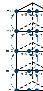
Figure 4.Vertical numbering of degrees of freedom (shown in filled circles) associated with vertices and horizontal edges. Only one set of vertically aligned degrees of freedom of each type is shown. The arrows outline the order in which the degrees of freedom are num-bered.

ing only cells for example). Degrees of freedom belonging to vertically adjacent entities, accessed by two consecutive ker-nel applications on the same column, have a constant offset between them. The offset is given by the sum of degrees of freedom attached to the two vertically adjacent entities con-tained in the stencil:

δ((d,0))+δ((d,1)). (8)

Let S be the stencil of a kernel which needs to access the values of the degrees of freedom of a fieldf defined on a function space fs. LetL_fs(v)=(dof₀,dof₁, . . .,dofk₋₁)be the list of degrees of freedom of the stencil for an input entity v∈Vd1,d2.

The lists of degrees of freedom accessed byS could be provided explicitly for all the input entitiesv. Using the pre-vious result we can instead reduce the number of explicitly provided lists by a factor ofλ. For each column we visit, the only explicit accesses required are the ones to the degrees of freedom at the bottom of the column. The degrees of freedom identifiers for the rest of the stencil applications in the same column can be obtained by adding a multiple of the constant vertical offset to each degree of freedom in the bottom ex-plicit list.

For a given stencil functionS an offset can be computed for each degree of freedom in the corresponding explicit list L_fs. As the ordering of the degrees of freedom in the stencil is fixed (by consistent ordering of mesh entities) the vertical offset only needs to be computed once for a particular func-tion spacef s.

(6)

ver-3808 G.-T. Bercea et al.: A numbering algorithm for finite elements on extruded meshes 6 G.-T. Bercea et al.: A numbering algorithm for finite elements on extruded meshes

Lfs. As the ordering of the degrees of freedom in the stencil

is fixed (by consistent ordering of mesh entities) the vertical offset only needs to be computed once for a particular func-tion spacef s.

The algorithm for computing the vertical offset is pre-5

sented in Algorithm 2. Note that since the offset for two ver-tically aligned entity types is the same, only the base mesh entity type is considered.

Algorithm 2Computation of vertical offsets

Require: k: number of degrees of freedom accessed by stencil

functionS

Require: ES(i): the base mesh entity type of thei-th degree of

freedom accessed byS

Require: δ((d₁, d₂)): the number of DoFs associated with each

(d₁, d₂)entity

Ensure: offsetS,fs: the vertical offset for function spacefsgiven

stencilS

foriin{0,1, ..., k−1}do d←ES(i)

offsetS,fs(i)←δ((d,0))+δ((d,1))

end for

Geosci. Model Dev., 9, 1–6, 2016 www.geosci-model-dev.net/9/1/2016/

tically aligned entity types is the same, only the base mesh entity type is considered.

If(dof₀,dof₁, . . .,dofk₋₁)is the explicit list of degrees of freedom for the initial layer to which the stencil can be ap-plied, then the list of degrees of freedom for thenth applica-tion of the stencil along the vertical is given by

(dof₀+n×(offsetS,f(0)), . . .,dofk₋₁

+n×(offsetS,f(k−1))). (9)

Algorithm 3 shows the iteration algorithm working for a single fieldf on a function space fs. The stencil functionS is applied to the entities of each column in turn. Each time the algorithm moves on to the next vertically adjacent entity, the indices of the degrees of freedom accessed are incremented by the vertical offset offsetS,fs. The algorithm is also applica-ble to stencil functions of multiple fields defined on the same function space since the data associated with each field are accessible using the same set of degree of freedom numbers. The extension to fields from different function spaces just re-quires explicit listsL_fsfor each space.

4 Performance evaluation

In this section, we test the hypothesis that iteration exploiting the extruded structure of the mesh amortizes the unstructured base mesh overhead of accessing memory through explicit neighbour lists. We also show that the more layers the mesh contains, the closer its performance is to the hardware limits of the machine.

We validate our hypotheses in the Firedrake finite element framework (Rathgeber et al., 2016). Although we restrict our performance evaluation to examples drawn from finite ele-ment discretizations, the algorithms we have presented can be applied to any mesh-based discretization.

In Sect. 4.1 we describe the design of the experiments un-dertaken. The hardware platforms and the methodology used are described in Sect. 4.2 followed by results and discussion in Sects. 4.3 and 4.4 respectively.

6 G.-T. Bercea et al.: A numbering algorithm for finite elements on extruded meshes Lfs. As the ordering of the degrees of freedom in the stencil

Algorithm 2Computation of vertical offsets

Require: k: number of degrees of freedom accessed by stencil

functionS

Require: E_S(i): the base mesh entity type of thei-th degree of

freedom accessed byS

Require: δ((d1, d2)): the number of DoFs associated with each

(d1, d2)entity

Ensure: offset_S,_fs: the vertical offset for function spacefsgiven

stencilS

foriin{0,1, ..., k−1}do d←ES(i)

offsetS,fs(i)←δ((d,0))+δ((d,1))

end for

Lfs. As the ordering of the degrees of freedom in the stencil

If(dof0,dof1, . . .,dofk₋1)is the explicit list of degrees of

freedom for the initial layer to which the stencil can be ap-10

plied, then the list of degrees of freedom for thenth

applica-tion of the stencil along the vertical is given by:

(dof₀+n×(offsetS,f(0)), . . .,dofk₋₁+n×(offsetS,f(k−1)))

(9)

Algorithm 3 shows the iteration algorithm working for a single fieldf on a function spacefs. The stencil functionS

15

is applied to the entities of each column in turn. Each time the algorithm moves on to the next vertically adjacent entity, the indices of the degrees of freedom accessed are incremented by the vertical offsetoffsetS,fs. The algorithm is also

appli-cable to stencil functions of multiple fields defined on the 20

same function space since the data associated with each field is accessible using the same set of degree of freedom num-bers. The extension to fields from different function spaces just requires explicit listsLfsfor each space.

Algorithm 3Iteration of a stencil function over an extruded mesh

Require: V: iteration set of base mesh entities

Require: d₂: the dimension of vertical iteration entities

Require: λ: the number of vertical intervals

Require: S: stencil function to be applied to the degrees of freedom

of fieldf

Require: L_fs: set of explicit lists of degrees of freedom for

func-tion spacefs

Require: offsetS,fs: the vertical offset for function spacefsgiven

stencilS

forvinVdo

(dof0,dof1, ...,dofk₋1)_←L_fs(v)

forlin{0,1, ..., λ−d₂}do

S(f (dof₀), f (dof₁), ..., f (dofk₋₁))

forjin{0,1, ..., k−1}do

dofj←dofj+offsetS,fs(j )

end for end for end for

4.1 Experimental design

The design space to be explored is parameterized by num-ber of layers and the manner in which the data are associ-ated with the mesh and therefore accessed. In establishing the relationship between the performance and the hardware we examine performance on two generations of processors and varying process counts.

4.1.1 Choosing the computation

Numerical computations of integrals are the core mesh iter-ation operiter-ation in the finite element method. We focus on residual (vector) assembly for two reasons. First, in contrast to Jacobian assembly, there are no overheads due to sparse matrix insertion; the experiment is purely a test of data ac-cess via the mesh indirections. Second, residual evaluation is the assembly operation with the lowest computational inten-sity and therefore constitutes a worst-case scenario for data layout performance exploration.

Since we are interested in data accesses, we choose the simplest non-trivial residual assembly operation:

I₁= Z

f vdx, ∀v∈V (10)

forf in the finite element spaceV. For this study we choose = [0,1]3to be the unit cube. The base mesh is generated in an unstructured manner using Gmsh (Geuzaine and Remacle, 2009), and then extruded to form a three-dimensional do-main.

In addition to the output fieldI₁and the input fieldf this computation accesses the coordinate field,x. Regardless of

(7)

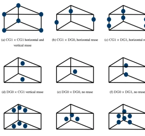
Figure 5.Tensor product finite elements with different data layout and cell-to-cell data re-use.

4.1.2 Choosing the discretizations

The construction of a wide variety of finite element spaces on extruded meshes was introduced in McRae et al. (2016). This enables us to select the horizontal and vertical data dis-cretizations independently.

For the purposes of data access, the distinguishing feature of different finite element spaces is the extent to which de-grees of freedom are shared between adjacent cells.

We choose a set of finite element spaces spanning the com-binations of horizontal and vertical reuse patterns found on extruded meshes: horizontal and vertical reuse, only horizon-tal, only vertical, or no reuse at all.

We employ low-order continuous and discontinuous dis-cretizations (abbreviated asCGandDGrespectively) in both

the horizontal and vertical directions.

The set of discretizations isA= {CG1,DG0,DG1}where the number indicates the degree of polynomials in the space. We examine all pairs of discretizations(h, v)∈A×A. Since the cells of the base mesh are triangles, the extruded mesh consists of triangular prisms. Figure 5 shows the data layout of each of these finite elements.

Both Firedrake and our numbering algorithm support a much larger range of finite element spaces than this. How-ever, the more complex and higher degree spaces will result in more computationally intensive kernels but not materially different data reuse. The lowest-order spaces are the most se-vere test of our approach since they are more likely to be memory bound.

Table 2.Hardware used.

Name Intel Sandy Bridge Intel Haswell

Model Xeon E5-2620 Xeon E5-2640 v3

Frequency 2.0 GHz 2.6 GHz

Sockets 2 2

Cores per socket 6 8

Bandwidth per socket 42.6 GB s−1 56.0 GB s−1

4.1.3 Layer count and problem size

We vary the number of layers between 1 and 100. This is a realistic range for current ocean and atmosphere simulations. The number of cells in the extruded mesh is kept approxi-mately constant by shrinking the base mesh as the number of layers increases. The mesh size is chosen such that the data volume far exceeds the total last level cache capacity of each chosen architecture (L3 cache in all cases). This minimizes caching benefits and is therefore the strongest test of our al-gorithms. The overall mesh size is fixed at approximately 15 million cells, which yields a data volume of between 300 and 840 MB, depending on discretization.

4.1.4 Base mesh numbering

The order in which the entities of the unstructured mesh are numbered is known to be critical for data access perfor-mance. To characterize this effect and distinguish it from the impact of the number of layers, we employ two variants of each base mesh. The first is a mesh for which the traversal is optimized using a reverse Cuthill–McKee ordering (Lange et al., 2016). The second is abadlyordered mesh with a

ran-dom numbering. This represents a pathological case for tem-poral locality.

4.2 Experimental setup

The specification of the hardware used to conduct the experi-ments is shown in Table 2. Following Ofenbeck et al. (2014) we disable the Intel turbo boost and frequency scaling. This is intended to prevent our performance results from being subject to fluctuations due to processor temperature.

The experiments we are considering are run on a single two-socket machine and use MPI (Message Passing Inter-face) parallelism. The number of MPI processes varies from one up to two processes per physical core (exploiting hy-perthreading). We pin the processes evenly across physical cores to ensure load balance and prevent process migration between cores.

The Firedrake platform performs integral computations by automatically generatingCcode. The compiler used is GCC

(8)

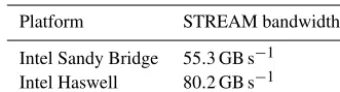
Table 3. Maximum STREAM triad (ai=bi+αci) performance

achieved by varying the number of MPI processes from one to twice the number of physical cores.

Platform STREAM bandwidth

Intel Sandy Bridge 55.3 GB s−1

Intel Haswell 80.2 GB s−1

in this paper since the performance of the Intel compiler was inferior.

4.2.1 Runtime, data volume, bandwidth, and FLOPs Runtime is measured using a nanosecond precision timer. Each experiment is performed 10 times and we report the minimum runtime. Exclusive access to the hardware has been ensured for all experiments.

We model the data transfer from main memory to CPU assuming a perfect cache: each piece of data is only loaded from main memory once. We define the valuable data vol-ume as the total size of the input, output, and coordinate

fields. This gives a lower bound on the memory traffic to and from main memory. The valuable data volume divided by the runtime yields thevaluable bandwidth.

Different discretizations lead to different data volumes due to the way data are shared between cells. DG-based dis-cretizations require the movement of larger data volumes, while CG discretizations lead to smaller volumes due to data reuse.

To evaluate the impact of different data volumes we com-pare the valuable bandwidth with the maximum bandwidth achieved for the STREAM triad benchmark (McCalpin, 1995), shown in Table 3. The valuable bandwidth achieved as a percentage of STREAM bandwidth shows how prone the code is to becoming bandwidth bound as its floating point performance is improved.

The floating point operations – adds, multiplies, and, on Haswell, fused multiply–add (FMA) operations – are counted automatically using the Intel Architecture Code Analyzer (Intel, 2012) whose results are verified with PAPI (Mucci et al., 1999) which accesses the hardware coun-ters.

4.2.2 Theoretical performance bounds

The performance of the extruded iteration depends on the ef-ficiency of the generated finite element kernel (payload) code which for some cases may not be vectorized (as outlined in Luporini et al., 2015) or may not have a perfectly balanced number of floating point additions and multiplications. A dis-cussion of kernel code optimality is outside the scope of this paper.

To a first approximation the performance of a numerical algorithm will be limited by either the memory bandwidth

or the floating point throughput. The STREAM benchmark provides an effective upper bound on the achievable memory bandwidth. The floating point bounds employed are based on the theoretical maximum given the clock frequency of the processor.

The Intel architectures considered are capable of executing both a floating point addition and a floating point multiplica-tion on each clock cycle. The Haswell processor can execute a fused multiply–add instruction (FMA) instead of either an addition or multiplication operation.

The achievable FLOP rate may therefore be as much as twice the clock rate depending on the mix of instructions ex-ecuted. The achievable speed-up over the clock rate,f_b, for the Sandy Bridge platform is therefore bounded by the bal-ance factor

f_b=1+ min(add FLOPs,multiplication FLOPs)

max(add FLOPs,multiplication FLOPs), (11) while for Haswell it is bounded by

f_b=1+min(add FLOPs,multiplication FLOPs)+k max(add FLOPs,multiplication FLOPs)+k, (12) wherekis half the number of FMAs.

4.2.3 Vectorization

The processors employed support 256 bit wide vector float-ing point instructions. The double precision FLOP rate of a fully vectorized code can be as much as 4 times that of an unvectorized code. GCC automatically vectorized only a part of the total number of floating point instructions. The ratio between the number of vector (packed) floating point instructions and the total number of floating point instruc-tions (scalar and packed) characterizes the impact of partial vectorization on the floating point bound through the vector-ization factor

f_v=1+(4−1)×vector FLOPs

total FLOPs . (13)

To control the impact of the kernel computation (payload) on the evaluation, we compare the measured floating point throughput with a theoretical peak which incorporates the payload instruction balance and the degree of vectorization. Letcbe the number of active physical CPU cores during the computation of interest. The theoretical base floating point performanceBc is the same for all discretizations and as-sumes one floating point instruction per cycle for each ac-tive physical CPU core. The peak theoretical floating point throughputPd is different for each discretizationd as it de-pends on the properties of the payload and is given by

(9)

0 20 40 60 80 100

Number of layers 0.0

1.0 2.0 3.0 4.0

Pe

rfo

rm

an

ce

[G

FL

O

P

S

]

E5-2620 Xeon Sandy Bridge EP

CG1xCG1 CG1xDG0 CG1xDG1 DG0xCG1 DG0xDG0 DG0xDG1 DG1xCG1 DG1xDG0 DG1xDG1

(a) Sandy Bridge, 1 process,c= 1

0 20 40 60 80 100

5.0 10.0 15.0 20.0 25.0

Pe

rfo

rm

an

ce

[G

FL

O

P

S

]

(b) Sandy Bridge, 6 processes,c= 6

0 20 40 60 80 100

10.0 20.0 30.0 40.0 50.0

Pe

rfo

rm

an

ce

[G

FL

O

P

S

]

(c) Sandy Bridge, 12 processes,c= 12

0 20 40 60 80 100

10.0 20.0 30.0 40.0 50.0

Pe

rfo

rm

an

ce

[G

FL

O

P

S

]

(d) Sandy Bridge, 24 processes,c= 12

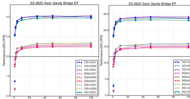
Figure 6.Performance of theIintegral computation with varying number of layers and number of processes on a badly-ordered base mesh. The horizontal line is the base FLOP throughput forfb=fv= 1and the number of physical cores used.

16

Figure 6.Performance of theIintegral computation with a varying number of layers and number of processes on a badly ordered base mesh.

The horizontal line is the base FLOP throughput forf_b=f_v=1 and the number of physical cores used.

4.3 Experimental results

4.3.1 Percentage of theoretical performance

For the Sandy Bridge and Haswell architectures, the best per-formance is achieved in the 100-layer case run with 24 and 32 processes respectively (hyperthreading enabled). The results in Tables 4 and 5 show percentages of the STREAM band-width and the theoretical floating point throughput which in-corporates the instruction balance and vectorization factors.

On Sandy Bridge, the proportion of peak theoretical float-ing point throughput is between 71 and 85 %, while on

Haswell it is between 71 and 92 %. In contrast, the propor-tion of peak bandwidth achieved varies between 7 and 51 % on Sandy Bridge and 9 and 75 % on Haswell. The higher and much more consistent peak FLOP results lead us to the con-clusion that we are in an operation- rather than bandwidth-limited regime. The performance figures are therefore pre-sented with respect to this metric.

4.3.2 Amortizing the cost of indirect accesses

(10)

0 20 40 60 80 100 Number of layers

0.0 1.0 2.0 3.0 4.0

Pe

rfo

rm

an

ce

[G

FL

O

P

S

]

(a) Sandy Bridge, 1 process,c= 1

0 20 40 60 80 100

5.0 10.0 15.0 20.0 25.0

Pe

rfo

rm

an

ce

[G

FL

O

P

S

]

(b) Sandy Bridge, 6 processes ,c= 6

0 20 40 60 80 100

10.0 20.0 30.0 40.0 50.0

Pe

rfo

rm

an

ce

[G

FL

O

P

S

]

(c) Sandy Bridge, 12 processes,c= 12

0 20 40 60 80 100

10.0 20.0 30.0 40.0 50.0

Pe

rfo

rm

an

ce

[G

FL

O

P

S

]

(d) Sandy Bridge, 24 processes,c= 12

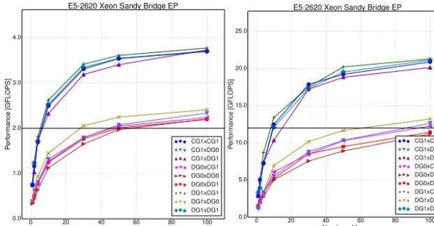
Figure 7.Performance of theIintegral computation with varying number of layers and number of processes on a well-ordered base mesh. The star-shaped markers show the performance of the 1-layer badly-ordered mesh for comparison. The horizontal line is the base FLOP throughput forfb=fv= 1and the number of physical cores used.

17

Figure 7.Performance of theIintegral computation with a varying number of layers and number of processes on a well-ordered base mesh.

The star-shaped markers show the performance of the one-layer badly ordered mesh for comparison. The horizontal line is the base FLOP throughput forf_b=fv=1 and the number of physical cores used.

and 20 for all discretizations. When the base mesh is badly ordered (Fig. 6) the plateau is frequently not reached even with 100 layers. A striking feature of Figs. 6 and 7 is that cases in which the local kernel calculations are identical pro-duce very similar achieved FLOP rates, despite having dif-ferent data sharing patterns. This supports the hypothesis that the results are operation bound.

4.4 Discussion

The performance of the extruded mesh iteration is con-strained by the properties of the mesh and the kernel

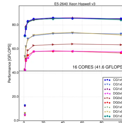
com-putation. The total number of computations is based on the number of degrees of freedom per cell. The range of dis-cretizations used in this paper (Fig. 5) leads to four cases: one, two, three, or six degrees of freedom per cell. In com-pute bound situations, discretizations with the same number of computations have the same performance (Fig. 8). Temporal locality

(11)

Table 4. Percentage of STREAM bandwidth and theoretical throughput achieved by the computation of integralIover 100

lay-ers on Sandy Bridge with 24 MPI processes.

Discretization f_b f_v Pd(%) Bandwidth (%)

CG1×CG1 1.7 1.58 73.45 7.092

CG1×DG0 1.81 1.0 78.96 14.70

CG1×DG1 1.7 1.58 73.03 10.50

DG0×CG1 1.65 1.0 76.01 27.86

DG0×DG0 1.5 1.0 85.14 34.86

DG0×DG1 1.65 1.0 75.45 45.68

DG1×CG1 1.7 1.58 73.20 24.60

DG1×DG0 1.81 1.0 78.93 50.98

DG1×DG1 1.7 1.58 71.78 44.37

Table 5. Percentage of STREAM bandwidth and theoretical throughput achieved by the computation of integralIover 100

lay-ers on Haswell with 32 MPI processes.

Discretization f_b f_v Pd(%) Bandwidth (%)

CG1×CG1 1.76 1.61 72.43 9.015

CG1×DG0 1.97 1.0 88.57 21.92

CG1×DG1 1.76 1.61 72.20 13.39

DG0×CG1 1.87 1.0 73.94 38.74

DG0×DG0 1.66 1.0 91.93 53.10

DG0×DG1 1.87 1.0 72.89 63.11

DG1×CG1 1.76 1.61 71.99 31.19

DG1×DG0 1.97 1.0 87.55 75.17

DG1×DG1 1.76 1.61 71.50 56.98

visits the next element. The reuse distance along the vertical is therefore minimal.

For CG discretizations, where degrees of freedom are shared horizontally with other vertical columns, the overall performance depends on the ordering of cells in the base mesh. Assuming a perfect ordering of the base mesh, the numbering algorithm ensures a minimal reuse distance while guaranteeing a minimum number of indirect accesses and satisfying all the previously introduced spatial and temporal locality requirements.

Figures 7 and 6 demonstrate the combined impact of hor-izontal mesh ordering and extrusion. In the extreme case the flop rate increases up to 14 times between the badly ordered single-layer case and the 100-layer well-ordered case. This is consistent with the widely held belief that unstructured mesh models are an order of magnitude slower than struc-tured mesh models.

The difference between well-ordered and badly ordered mesh performance outlines the benefits responsible for the boost in performance. Horizontal data reuse dominates per-formance for a low number of layers, while spatial locality and vertical temporal locality (ensured by the numbering and iteration algorithms) are responsible for most of the perfor-mance gains as the number of layers increases.

0 20 40 60 80 100 Number of layers

0.0 20.0 40.0 60.0 80.0

Pe

rfo

rm

an

ce

[G

FL

O

P

S

]

1 CORE (2.6 GFLOPS) BALANCED (5.2 GFLOPS) 16 CORES (41.6 GFLOPS) BALANCED (83.2 GFLOPS) E5-2640 Xeon Haswell v3

Figure 8.Performance of theIintegral computations on different

data discretizations with a varying number of layers on the Haswell architecture for a well-ordered base mesh. The star-shaped mark-ers show the performance of the one-layer badly ordered mesh for comparison. The horizontal line is the base FLOP throughput for

f_b=f_v=1 and the number of physical cores used.

We note, once again, that these results are for the lowest-order spaces which represent a worst case. Higher-lowest-order methods both access more contiguous data in each column and require many more FLOPs. As a result, we would expect to reach performance plateaus at lower numbers of layers.

5 Conclusions

In this paper we have presented efficient, locality-aware al-gorithms for numbering and iterating over extruded meshes. For a sufficient number of layers, the cost of using an unstruc-tured base mesh is amortized. Achieved performance ranges from 70 to 90 % of our best estimate for the hardware’s per-formance capabilities and current level of kernel optimiza-tion. Benefits of spatial and temporal locality vary with the number of layers: as the number of layers is increased, the benefits of spatial locality increase, while those of temporal locality decrease.

This paper employed two simplifying constraints: that there are a constant number of layers in each column, and that the number of degrees of freedom associated with each entity type is a constant. These assumptions are not funda-mental to the numbering algorithm presented here, or to its performance. We intend to relax those constraints as they be-come important for the use cases for which Firedrake is em-ployed.

(12)

be vectorized at intra-kernel level. The efficiency of such a generic scheme applicable to different data discretizations is currently being explored.

In future work we intend to generalize some of the opti-mizations which extrusion enables for both residual and Ja-cobian assembly: inter-kernel optimizations, grouping of ad-dition of contributions to the global system, and exploiting the vertical alignment at the level of the sparse representa-tion of the global system matrix. In addirepresenta-tion to the CPU re-sults presented in this paper, we also plan to explore the per-formance portability issues of extruded meshes on graphical processing units and Intel Xeon Phi accelerators.

6 Code availability

The packages used to perform the experiments have been archived using Zenodo: Firedrake (Firedrake, 2016), PETSc (PETSc, 2016), petsc4py (petsc4py, 2016), FIAT (FIAT, 2016), UFL (UFL, 2016), FFC (FFC, 2016), PyOP2 (PyOP2, 2016), and COFFEE (COFFEE, 2016). The source code repositories as well as the archived versions are publicly available.

7 Data availability

The scripts used to perform the experiments as well as the results are archived using Zenodo: Sandy Bridge (Bercea, 2016c) and Haswell (Bercea, 2016b). The meshes used in the experiments are available also (Bercea, 2016a). The archives are publicly available.

Author contributions. Gheorghe-Teodor Bercea designed the

gen-eralized extrusion algorithm, and performed the extension of the Firedrake and PyOP2 packages to support extruded meshes, the performance evaluation, and the preparation of the graphs and ta-bles. Andrew T. T. McRae extended components of the Firedrake toolchain to support the finite element types used in the experi-ments, and made minor contributions to the extruded mesh iteration functionality. David A. Ham was the proponent of a generalized extrusion algorithm. Lawrence Mitchell, Florian Rathgeber, and Fabio Luporini developed related features and framework improve-ments in Firedrake, PyOP2, and COFFEE. Luigi Nardi is responsi-ble for the use of the floating point balance metric. David A. Ham and Paul H. J. Kelly are the principal investigators for this paper. Gheorghe-Teodor Bercea prepared the manuscript with contribu-tions from all the authors. All authors contributed with feedback during the paper’s write-up process.

Acknowledgements. This work was supported by an

Engineer-ing and Physical Sciences Research Council prize studentship (ref. 1252364), the Grantham Institute and Climate-KIC, the Natu-ral Environment Research Council (grant numbers NE/K006789/1, NE/K008951/1, and NE/M013480/1) and the Department of

Computing, Imperial College London. The authors would like to thank J. (Ram) Ramanujam at Louisiana State University for the insightful discussions and feedback during the writing of this paper. We are thankful to Francis Russell at Imperial College London for the feedback on this paper.

Edited by: S. Unterstrasser

Reviewed by: two anonymous referees

References

Bercea, G.-T.: Unstructured meshes for extrusion article, doi:10.5281/zenodo.61819, 2016a.

Bercea, G.-T.: Data and plot scripts for Haswell experiments, doi:10.5281/zenodo.61919, 2016b.

Bercea, G.-T.: Data and plot scripts for Sandy Bridge experiments, doi:10.5281/zenodo.61920, 2016c.

COFFEE: A Compiler for Fast Expression Evaluation, doi:10.5281/zenodo.47715, 2016.

FFC: FEniCS Form Compiler, doi:10.5281/zenodo.47761, 2016.

FIAT: The Finite Element Automated Tabulator,

doi:10.5281/zenodo.47716, 2016.

Firedrake: An automated finite element system,

doi:10.5281/zenodo.47717, 2016.

Ford, R., Glover, M., Ham, D., Maynard, C., Pickles, S., and Riley, G.: GungHo Phase 1: Computational Science Recommendations, Tech. rep., Met Office, Exeter, 2013.

Gersbacher, C.: The Dune-PrismGrid Module, in: Advances in DUNE: Proceedings of the DUNE User Meeting, edited by: Dedner, A., Flemisch, B., and Klöfkorn, R., 6–8 October 2010, Stuttgart, Germany, 33–44, Springer Berlin Heidelberg, Berlin, Heidelberg, doi:10.1007/978-3-642-28589-9_3, 2012.

Geuzaine, C. and Remacle, J.-F.: Gmsh: A 3-D finite element mesh generator with built-in pre- and post-processing facilities, In-ternational Journal for Numerical Methods in Engineering, 79, 1309–1331, 2009.

Günther, F., Mehl, M., Pögl, M., and Zenger, C.: A Cache-Aware Algorithm for PDEs on Hierarchical Data Structures Based on Space-Filling Curves, SIAM J. Sci. Comput., 28, 1634–1650, doi:10.1137/040604078, 2006.

Intel: Intel Architecture Code Analyzer,

avail-able at: https://software.intel.com/en-us/articles/

intel-architecture-code-analyzer (last access: October 2016), 2012.

Isaac, T.: Scalable, adaptive methods for forward and inverse prob-lems in continental-scale ice sheet modeling, PhD thesis, Univer-sity of Texas, Austin, 2015.

Isaac, T., Stadler, G., and Ghattas, O.: Solution of Nonlinear Stokes Equations Discretized By High-Order Finite Elements on Nonconforming and Anisotropic Meshes, with Application to Ice Sheet Dynamics, SIAM J. Sci. Comput., 37, B804–B833, doi:10.1137/140974407, 2015.

Knepley, M. G. and Karpeev, D. A.: Mesh Algorithms for PDE with Sieve I: Mesh Distribution, Sci. Program., 17, 215–230, doi:10.3233/SPR-2009-0249, 2009.

(13)

J. Sci. Comput., available at: http://arxiv.org/abs/1506.07749, in press, 2016.

Logg, A.: Efficient Representation of Computational

Meshes, Int. J. Comput. Sci. Eng., 4, 283–295,

doi:10.1504/IJCSE.2009.029164, 2009.

Luporini, F., Varbanescu, A. L., Rathgeber, F., Bercea, G.-T., Ra-manujam, J., Ham, D. A., and Kelly, P. H. J.: Cross-Loop Optimization of Arithmetic Intensity for Finite Element Lo-cal Assembly, ACM Trans. Archit. Code Optim., 11, 1–25, doi:10.1145/2687415, 2015.

Macdonald, A. E., Middlecoff, J., Henderson, T., and Lee, J.-L.: A General Method for Modeling on Irregular Grids, Int. J. High Perform. C., 25, 392–403, doi:10.1177/1094342010385019, 2011.

McCalpin, J. D.: Memory Bandwidth and Machine Balance in Current High Performance Computers, IEEE Computer Soci-ety Technical Committee on Computer Architecture (TCCA) Newsletter, 19–25, 1995.

McRae, A. T. T., Bercea, G.-T., Mitchell, L., Ham, D. A., and Cot-ter, C. J.: Automated generation and symbolic manipulation of tensor product finite elements, SIAM J. Sci. Comput., available at: http://arxiv.org/abs/1411.2940, in press, 2016.

Meister, O. and Bader, M.: 2D adaptivity for 3D problems: Parallel SPE10 reservoir simulation on dynamically adaptive prism grids, J. Comput. Sci., 9, 101–106, doi:10.1016/j.jocs.2015.04.016, 2015.

Mucci, P. J., Browne, S., Deane, C., and Ho, G.: PAPI: A Portable Interface to Hardware Performance Counters, Proceedings of the Department of Defense HPCMP Users Group Conference, 7–10, 1999.

Ofenbeck, G., Steinmann, R., Caparros, V., Spampinato, D. G., and Puschel, M.: Applying the roofline model, in: 2014 IEEE Inter-national Symposium on Performance Analysis of Systems and Software (ISPASS), 76–85, doi:10.1109/ISPASS.2014.6844463, 2014.

PETSc: Portable, Extensible Toolkit for Scientific Computation, doi:10.5281/zenodo.47718, 2016.

petsc4py: The Python interface to PETSc,

doi:10.5281/zenodo.47714, 2016.

PyOP2: Framework for performance-portable parallel computations on unstructured meshes, doi:10.5281/zenodo.47712, 2016. Rathgeber, F., Ham, D. A., Mitchell, L., Lange, M., Luporini, F.,

McRae, A. T. T., Bercea, G.-T., Markall, G. R., and Kelly, P. H. J.: Firedrake: automating the finite element method by com-posing abstractions, ACM Trans. Math. Software, available at: http://arxiv.org/abs/1501.01809, in press, 2016.

Sarje, A., Song, S., Jacobsen, D., Huck, K., Hollingsworth, J., Malony, A., Williams, S., and Oliker, L.: Parallel

Per-formance Optimizations on Unstructured Mesh-based

Simulations, Procedia Computer Science, 51, 2016–2025, doi:10.1016/j.procs.2015.05.466, 2015.

Skamarock, W. C., Klemp, J. B., Duda, M. G., Fowler, L. D., Park, S.-H., and Ringler, T. D.: A multiscale nonhydro-static atmospheric model using centroidal Voronoi tesselations and C-grid staggering, Mon. Weather Rev., 140, 3090–3105, doi:10.1175/MWR-D-11-00215.1, 2012.

Slingo, J., Bates, K., Nikiforakis, N., Piggott, M., Roberts, M., Shaffrey, L., Stevens, I., Vidale, P. L., and Weller, H.: Devel-oping the next-generation climate system models: challenges and achievements, Philos. T. R. Soc. Lond. A, 367, 815–831, doi:10.1098/rsta.2008.0207, 2009.

UFL: The Unified Form Language, doi:10.5281/zenodo.47713, 2016.

Yoon, S.-E., Lindstrom, P., Pascucci, V., and Manocha, D.: Cache-oblivious Mesh Layouts, ACM Trans. Graph., 24, 886–893, doi:10.1145/1073204.1073278, 2005.