Using the Bernoulli trial approaches for detecting ordered alternatives

R E S E A R C H A R T I C L E

Open Access

Using the Bernoulli trial approaches for detecting

ordered alternatives

Chia-Hao Chang

, Chih-Chien Chin

, Weichieh Wayne Yu

and Ying-Yu Huang

Abstract

Background:Diagnostic problems in clinical trials are sometimes ordinal. For example, colon tumor staging was performed according to the TNM classification. However, clinical data are limited by markedly small sample sizes in some stage.

Methods:We propose a distribution-free test for detecting ordered alternatives in a completely randomized design. The new statistic is based on summing all correctly (ascending) ordered samples.

Results:The exact mean and variance of the null distribution are derived and it is shown that this distribution is asymptotically normal. Furthermore, we show using Monte Carlo simulation that the proposed test is a significant improvement over the Terpstra-Magel test. That is, power is decreased where the investigator falsely assumes an a priori ordering relationship.

Conclusions:We conclude that these tests frequently detect an ordered trend when, in fact, one does not exist. However, the new test can reduce the error rate, at least not to the extent in which the Jonckheere-Terpstra test does.

Background

This paper focuses on considering nonparametric tests for the non-decreasing ordered alternative of k(≥3) groups. The hypothesis to be tested isH0:F1(x) =F2(x) =⋯=Fk(x)

for all x andH1:F1(x)≥F2(x)≥ ⋯ ≥Fk(x), for all x with

F1(x) >Fk(x) for some x, whereF1(x),F2(x),⋯,Fk(x) are

continuous distribution functions.

In this article, we assume the location model withFi(x) =

F(x−μ−θi), whereμis a location parameter andθi

repre-sents the effect of group i, i = 1, 2, …, k. This

im-plies that the underlying populations may differ only in location. Throughout the article, let xi1; xi2;…;xini;

i ¼ 1; 2; …; k represent independent random

sam-ples from the kpopulations with distribution functions

Fi(x),i = 1, 2, …, k, respectively.

Nonparametric order restricted inference has been ex-tensively investigated in past literature and new studies are continuing to emerge. For instance, Puri [1], Puri and Sen [2], and Padmanabhan et al. [3] applied the con-cept of Chernoff–Savage-type statistics to nonparametric

ordered alternative tests. Studies that used power results to compare the validity of linear rank tests included Büning and Kössler [4], Beier and Büning [5], Büning and Kössler [6], Büning [7], Büning and Kössler [8], Büning and Kössler [9], Kössler [10] and Kössler [11].

The earliest and most classic treatment ofk(≥ 3)-sam-ple distribution-free statistic for ordered alternatives was proposed by Jonckheere [12] and Terpstra [13]. The test is known as the Jonckheere-Terpstra test (hereafter referred to as the JT test) and is based on a sum of Ck2 Mann– Whitney statistics (Mann and Whitney, [14]; Hollander and Wolfe, [15]). In order to define the JT statistic, we express the Mann–Whitney statistics as

Ulm¼ Xnl

jl¼1

Xnm

jm¼1

I xljl;xmjm

; 1≤l<m≤k;

whereI xljl;xmjm

¼ 1; if xljl<xmjm

0; otherwise

, and the JT statistic

is given byJT¼X

k−1

l¼1

Xk

m¼lþ1 Ulm.

Other tests for ordered alternatives were developed by Cuzick [16] and Le [17]. Among the JT, Cuzick, and Le

* Correspondence:[email protected] 1

Department of Nursing, Chang Gung University of Science and Technology, Chiayi Campus, Chiayi, Taiwan 61363

Full list of author information is available at the end of the article

tests, the results from Mahrer and Magel [18] did not establish any of the tests as having overwhelmingly higher power over the others across different location parameters. Neuhauser et al. [19] presented a modified version of the JT test (hereafter referred to as the MJT test). The form of the MJT statistic is identical to the JT test except that the Mann–Whitney statistic Ulm

multi-plies the weight m - las the new kernel. Study results

showed that the MJT test often produced a higher power than the JT test for the ordered alternative. We also noted that Tryon and Hettmansperger [20] presented the JT and MJT tests as members of a more general class of nonparametric tests. In the test statistics described above the kernels of the tests are almost all derived by comparing two pairs of sample observations at a time. However, Terpstra and Magel [21] proposed a test (here-after referred to as the TM test) where the kernels of TM test are based on information obtained simultan-eously across all samples. The statistic is determined by

adding theY

k

i¼1

niindicator functions, that is,

TM¼X

n1

j1¼1 ⋯Xnk

jk¼1

I x1j1≤x2j2≤⋯≤xkjk

where I x1j1≤x2j2≤⋯≤xkjk

is equal to one, provided at least one strict inequality; otherwise,I x1j1≤x2j2≤⋯≤xkjk

is equal to zero..

Terpstra et al. ([22]a, b) proposed a new nonparametric test statistic (hereafter referred to as the KTP test) that is a generalization of the TM test. The idea is to replace the indicator kernel from the TM test with Spearman’s rank correlation coefficient, that is,

KTP¼X

n1

j1¼1 ⋯Xnk

jk¼1

r x1j1;x2j2;…;xkjk

;

where is Spearman’s rank correlation coefficient between the observed data and the corresponding group number.

In this study, we propose a new test is based on the

in-formation present in the N¼Y

k

i¼1

ni k-tuplets, where a

k-tuplet includes one observation from each treatment group. All correctly (ascending) ordered samples are then summed to form a statistic that is distributed approxi-mately as a normal distribution. Details of this new test and its asymptotic distribution are provided, and the com-putational algorithm is presented in the Additional file 1. A colon cancer data example is given in data example sec-tion. Finally, we present a finite sample simulation study which compares the proposed test, the JT test, MJT test, TM test, and the KTP test in terms of power. A computer program written in R that implements the proposed

methods will be available from the first author upon re-quest. It is recommended that readers who are not inter-ested in the details of the computational algorithm skip the Additional file 1.

Methods

Test statistic

The new nonparametric test for non-decreasing alterna-tives is based on the following statistic,

T¼X

n1

j1¼1 ⋯Xnk

jk¼1

k x1j1;x2j2;…;xkjk

;

Where k xð 1;x2;…;xkÞ ¼

X_k

i¼1I R xð ð Þ ¼i iÞ, R (xi) de-notes the rank of xiwith respect to x1, x2,…, xk, and I(.) denotes the indicator function.

The remainder of this section presents and derives re-sults pertaining to the null distribution of the proposed test statistic. We assume throughout this section that the observed data, {Xij} is essentially a random sample from some continuous probability distribution function F. Hence, the possibility of ties has a probability of zero. In principle the test statistic uses the k-tuplet method of Terpstra and Magel. Additionally, in the null hypothesis each k x1j1;x2j2;…;xkjk

follows the Binomial (k, 1/k) distribution. For these reasons, we will refer to this test as the KTMB test.

The exact null distribution

Let N denote the sum of the sample sizes for each

treat-ment. Namely, let N=n1+⋯+nk. Here, we have N!/

(n1!⋯nk!) partitions of the numbers 1,…, N. The null

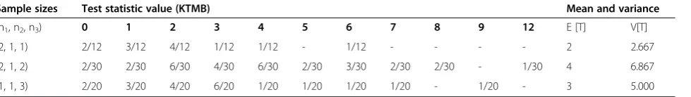
distribution of T means each one of these partitions is equally likely so the mean and variance can be calculated directly by multiplying each possible value of T with its probability. When the number of partitions is small, we can easily calculate the exact distribution by hand or with the computer. Table 1 shows the probabilities, means, and variances of the test statistic T for sample size arrangements (2, 1, 1), (2, 1, 2), and (1, 1, 3) respectively.

The mean and variance

If the asymptotic null distribution of a test statistic is normal and the exact mean and variance of T under H0 in standard form can be established we can then standardize T by using the exact mean and variance to obtainZKTMB, where ZKTMB¼fT−E0ð ÞT g=

ffiffiffiffiffiffi

V0

p

T ð Þ. In this case, we can find critical values from the standard normal table.

We will start by finding the mean value of T, E0(T),

noting that T is nothing but a sum of the kY

k

i¼1 ni

Bernoulli (1/k) distribution. It is straightforward to get

E0ð Þ ¼T

Yk

i¼1

ni ð1Þ

Here, and in the following, we letn¼Y

k

i¼1 ni;

V0ð Þ ¼T v20þ

Xk−1

i¼1

v2i þv2k ð2Þ

where v2

0¼f1−ð1=kÞg

Yk

i¼1

ni for no tie, v2k ¼ nk kð −1Þ

k−2

ð Þ!=k!−1=k2

for k ties for i≠j.

For the case of ities, we present an algorithm for the

computation of the X

k−1

i¼1

v2_i in Additional file 1. Readers

who are not interested in the details of this algorithm may want to skip the Additional file 1 and go to data ex-ample section, in which exex-amples based on real data are provided.

The asymptotic null distribution

In this section we will look to see if the asymptotic null distribution of test statistic T follows the standard nor-mal distribution. In other words, we prove that

T¼T−ffiffiffiffiffiffiffiffiffiffiffiffiffiffiE0ð ÞT V0ð ÞT

p →D

Nð0;1Þ: ð3Þ

H0will therefore be rejected for large values ofT*. The

normal approximation for the procedure is to rejectH0

if T*≥z1−α; otherwise do not reject H0. Note that the

critical value z1−α is chosen to make the Type I error probability equal to α. That is, α≈P(T*≥z1−α|H0true). We note that (3) is a direct consequence of Theorem 1, which we now state.

Theorem 1 Let N ¼X

k

l¼1

nl and assume nNl¼λlþoð Þ1

whereλl∈(0, 1). Then, under H0; TN¼ def ₁

k⋅Nk−1=2

Xn1

j1¼1 ⋯Xnk

jk¼1

k x1j1;⋯;xkjk

−1

→DN 0;X

k

l¼1

λ

lσ2lk !

;whereλ l ¼λl

Yk

j¼1

λ2I jð Þ≠l

j :

Proof of Theorem 1 Terpstra and Magel [21] proved

thatTMstatistic follows a normal distribution as sample sizes go to infinity by using projection technique from Hettmansperger and McKean ([23], p. 81). In what fol-lows all limits are taken with respect toN, asN→∞. To apply their theorem to our case, let

E½TNjXlm ¼

1 k⋅Nk−1=2

Xn1

j1¼1

⋯Xnk

jk¼1

Xk

i¼1

½Ii jl¼m

Zlk

ðXlmÞ þIi jl≠m

1

k− 1 k ¼

Lnð Þl

Nk−1=2 ZlkðXlmÞ−

1 k

where ZlkðXlmÞ ¼

def ð_k−₁Þ!

l−1 ð Þ!ðk−lÞ!F

l−1_{ð Þx½1−F xð Þ}k−l_;

l ¼ 1;…; k:

Lnð Þ ¼l Yk

j¼1 nI jjð Þ≠l:

The projection ofTN, say,PNcan be defined as,

PN ¼

Xk

l¼1

Xnl

m¼1

E½TNjXlm

¼Xk

l¼1

Lnð Þl ffiffiffiffinl

p

Nk−1=2

1

ffiffiffiffi

nl

p Xnl

m¼1

ZlkðXlmÞ−

1 k

:

ð4Þ

E Z½ lkðXlmÞ ¼1_k and V Z½ lkðXlmÞ ¼σ2lk can be proved

by Beta distribution. The convergence criteria on the k

sample sizes imply that,

Lnð Þl pffiffiffiffinl

Nk−1=2 ¼

ffiffiffiffiffi

λ

l q

þoð Þ1 : ð5Þ

Table 1 Some exact null distributions for the proposed test statistic

Sample sizes Test statistic value (KTMB) Mean and variance

(n1, n2, n3) 0 1 2 3 4 5 6 7 8 9 12 E [T] V[T]

It now follows from (4), (5), and limiting moment gen-erating function theory that,

PN→D N 0;

Xk

l¼1 λ

lσ2lk !

: ð6Þ

Let us now considerV[TN], which we write as,

V T½ N ¼

1 k2N2k−1

Xn1

i1¼1 ⋯Xnk

ik¼1

Xn1

j1¼1 ⋯Xnk

jk¼1

COV k xð 1i1;⋯;xkikÞ;k x1j1;⋯;xkjk

:

ð7Þ

Consider first the case ofkties fori≠j. it is

straightfor-ward to show COV k xð 1i1;⋯;xkikÞ; k x1j1;⋯;xkjk

¼k

k−1 ð Þ ðk−2Þ!

k! − 1 k2

h i

. Next, consider the case in which

there are exactly three ties among the different

sub-scripts. For example, if we let Ru denotes the rank of

xu with respect to x1, x2,…, xk, Rv denotes the rank of

xv with respect to x1, x2,…, x2k-3, u <v-k, Ru< Rv, and

X1, X2, X3 denote the tied observations then the

covariance term has the form COV [Iu, Iv] where, Ru

denotes the rank of xu with respect to X4;…;Xl1; X1; Xl1þ1;…;Xu;…;Xl2; X2;Xl2þ1;…;Xl3; X3;Xl3þ1…;Xk and Iu=I(Ru=u), and Rv denotes the rank of xv with

respect to Xkþ1;…;Xkþl1−3;X1;Xkþl1−2;…;Xkþl2−3;X2; Xkþl2−2;…;Xv;…;Xkþl3−3;X3;Xkþl3−2;…;X2k−3 and Iv= I(Rv=v).

Under H0, E I½ ¼u E I½ ¼v 1_k. Next, consider E [IuIv].

This expectation contains 2k-3 observations, so that

underH0, each of the (2k-3)! permutations of the

observa-tions are equally likely. However, there are only the num-bers of{1 : Ru-1}∩{1 : Rv-1}possible ways, sayISS(Ru, Rv),

plus the numbers of{Ru+1 : 2k-3}∩{1 : Rv-1}possible ways,

sayILS(Ru,Rv), plus the numbers of{Ru+1 : 2k-3}∩{Rv+1 :

2k-3}possible ways, sayILL(Ru,Rv), to preserveX1,X2, and

X3. Furthermore, there are CISSRu;Rv

ð Þ−t1

u−4 possible ways to

preserve X4;…;Xl1;Xl1þ1;…;Xu−1 to the left of Xu, CILSðRu;RvÞ−t2

v−k−1−ðu−4Þ possible ways to preserve Xkþ1;…;Xkþl1−3; Xkþl1−2;…;Xkþl2−3;Xkþl2−2; Xv−1 to the left of Xv, CILLðRu;RvÞ−t3

k−u−fILS−1−½v−k−1−ðu−4Þgpossible ways to preserveXuþ1;…; Xl2;Xl2þ1;…;Xl3; Xl3þ1…;Xk to the right of Xu, and CILLðRu;RvÞ−1−ðk−u−ILSþ1þv−k−1−uþ4Þ

ILLðRu;RvÞ−1−ðk−u−ILSþ1þv−k−1−uþ4Þ¼1 possible way to pre-serve Xvþ1;…;Xkþl3−3;Xkþl3−2;…X2k−3 to the right ofXv. Hence, these arguments imply that,

wheret1+t2+t3= 3,t1,t2, andt3= 0, 1, 2, 3.

Now, for a given l1, l2, and l3, there are nl1nl2nl3

Yk

t¼1 ntðnt−1Þ

½ I tð≠l1ÞI tð≠l2ÞI tð≠l3Þ

of these covariance terms. Next, consider all possible_Ru,Rvand all possible treatment

lo-cations (m and n), in the case of one tieX1, (7) reduces

to,

Xk

l¼1

nl Yk

t¼1

ntðnt−1Þ

½ I tð≠lÞ

N2k−1

X k−iþm

Ru¼m

X k−iþn

Rv¼n ½CISSRu;Rv

ð ÞþILSðRu;RvÞþILLðRu;RvÞ

t1þt2þt3 1

ðk−2Þ!ðk−2Þ!C

ISSðRu;RvÞ−t1 u−4 CILSRu;Rv

ð Þ−t2

v−k−1−ðu−4ÞCIkLL−uðR−ufI;RLSvðÞ−Rtu3;RvÞ−t2−½v−k−1−ðu−4Þg 2k−1

ð Þ! −

1

k2

¼Xk

l¼1 λ

lσ2lkþoð Þ1

ð8Þ

wheret1+t2+t3= 1,t1,t2, andt3= 0, 1.

From (6) and (8) it follows that V[TN]−V[PN] =o(1).

Asymptotic normality results are attainable.

Patient characteristics

The institutional review board of Chang Gung Memorial Hospital approved the present study. Detailed information about patients with colon cancer, such as patient- and tumor-related factors and follow-up status, was retrieved from the Colorectal Section Tumor Registry at Chang Gung Memorial Hospital, Taiwan. All the data in this registry were prospectively collected.

Results and discussion

Data examples

Between January 2006 and December 2010, 154 con-secutive patients with histologically confirmed colonic adenocarcinoma underwent curative surgeries at the Chang Gung Memorial Hospital in Chiayi. The stage IV colon cancer, non-curative surgeries, rectal cancer and mucinous adenocarcinomawere excluded in this study. Tumor staging was performed according to the TNM classification described in the 6th edition of the cancer staging manual of the American Joint Committee on Cancer (Stage I, II, IIIA and IIIB). The different tumor staging require a different treatment to optimize patient and hospital outcomes. An ordinal logistic regression model was developed with predictors as follows: age, gen-der, tumor location, histologic differentiation, preoperative

COV Ið u;IvÞ ¼

3!ðk−4Þ!ðk−4Þ!CISSðRu;RvÞþILSðRu;RvÞþILLðRu;RvÞ

t1þt2þt3 ⋅C

ISSðRu;RvÞ−t1 u−4 2k−3

ð Þ!

CILSðRu;RvÞ−t2

v−k−1−ðu−4ÞCILLRu;Rv ð Þ−t3

albumin level, preoperative carcinoembryonic antigen level, and underlying medical illnesses.

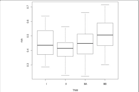
To illustrate the KTMB test, assume an outcome with four stages and a set of cases consisting of one case from each stage. The case from Stage I has risks of 0.50, 0.25, 0.15 and 0.10 for Stage I, II, IIIA and IIIB, respectively. The case from Stage II has risks 0.26, 0.52, 0.17 and 0.05; the case from Stage IIIA has risks 0.06, 0.32, 0.42 and 0.20; the case from Stage IIIB has risks 0.12, 0.18, 0.30 and 0.40. The risk for Stage IIIB (say, event) is higher for the case that belongs to this stage (0.40) than for the other cases (0.10, 0.05 and 0.20). The risk for event is second-highest for the case from Stage IIIA (0.20 versus 0.10, 0.05 and 0.40). However, the risk for event is lowest for the case from Stage II (0.05 versus 0.10, 0.20 and 0.40). The risk for event is third-highest for the case from Stage I (0.10 versus 0.05, 0.20 and 0.40). Therefore, the risks correctly identify the cases

from Stage IIIA and IIIB but not Stage I and II, resulting in a score of 2 for this set (k(x1,x2,x3,x4)).

Hence, the set of hypotheses was H0:FI(x) =FII(x) =

FIIIA(x) =FIIIB(x) for all x and H1:FI(x)≥FII(x)≥FIIIA

(x)≥FIIIB(x), whereFI(x)≠FIIIB(x) for some x.

Five test statistics and the corresponding p-values are given in Table 2. Since a plot of this data set in Figure 1 exhibits a non-increased trend, it appears that the JT, MJT and KTP tests have falsely conclusion (p < 0.05). The KTMB test has the largest p-value (See Table 2). Moreover, Stage IIIB patients reported significantly more risk for Stage IIIB than Stage II subjects (ANOVA, post hoc: IIIB > II, p = 0.003) while Stage I, II and IIIA pa-tients did not differ in risk for Stage IIIB (ANOVA, post-hoc: p>0.05) Hence, we conclude that the risk for Stage

IIIB do not increase with the patient’s TNM in the

model. That is, the discrimination performance of the ordinal logistic model is not very well between Stage I, II and IIIA.

Comparison with respect to size and power

To determine if the underlying population came from different skew and kurtosis distributions that impact on the power of the test statistic, we used log-F distribu-tions with combinadistribu-tions of 2, 4.5 and 10 degrees of

Table 2 Order restricted inference results for the colon cancer data

JT MJT TM KTP KTMB

Test Statistic 3.01 2.69 1.44 2.17 1.29 p-value 0.00132 0.00361 0.07473 0.01483 0.09830

I II IIIA IIIB

0

.3

0

.4

0

.5

0

.6

0

.7

TNM

ri

s

k

freedom to generate the random variable. We can there-fore define random variable Xij as:Xij=θi+εij, whereεij

is the iid log-F distribution, and θi are location

parameters.

For the numbers of treatment (k), sample sizes (ni)

and location parameters (θi) we examine the different

combinations of k = 3 and 4, ni= 4, 5, 8 and 10,θi = 0,

0.25, 0.5, 0.75, 1 and 1.25. We investigated designs under assumed alternatives which are of the forms of concave and convex. Programs to compare powers were written in R 2.9.2 (R Development Core Team, Vienna, Austria).

The estimations were conducted by simulating 10,000 different sets of samples. Furthermore, we estimated the

power by counting the number of times H0was rejected

and using the value to divide by 10,000. Ideally, we be-lieve that the test should have higher power than a

gen-eral alternative test when H1 is true, and should have

low power for any alternative that does not fit the profile given in H1.

In general, the JT and KTP tests have the highest pow-ers for the ordered alternative cases. Comparing with TM test, the gain percentage in power, DP = (KTMB

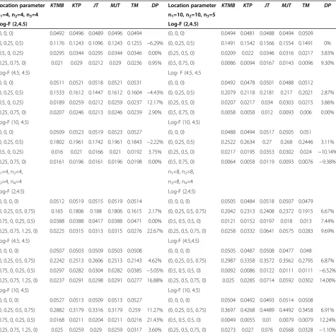
-Table 3 Estimated powers and type I error rates of ordered tests under significance level 0.05

Location parameter KTMB KTP JT MJT TM DP Location parameter KTMB KTP JT MJT TM DP

n1=4, n2=4, n3=4 n1=10, n2=10, n3=5

Log-F (2,4.5) Log-F (2,4.5)

(0, 0, 0) 0.0492 0.0496 0.0489 0.0496 0.0494 (0, 0, 0) 0.0494 0.0481 0.0488 0.0494 0.0509 (0, 0.25, 0.5) 0.1176 0.1243 0.1096 0.1243 0.1255 −6.29% (0, 0.25, 0.5) 0.1491 0.1542 0.1566 0.1554 0.1491 0% (0.5, 0, 0.25) 0.0295 0.0344 0.0295 0.0344 0.0346 0.00% (0.25, 0.5, 0) 0.0209 0.022 0.0346 0.0316 0.0217 3.83% (0.25, 0.75, 0) 0.021 0.029 0.0212 0.029 0.0236 0.95% (0.5, 0.75, 0) 0.0086 0.0094 0.0167 0.0143 0.0096 9.30% Log-F (4.5, 4.5) Log- F (4.5, 4.5

(0, 0, 0) 0.0511 0.0521 0.0518 0.0521 0.0531 (0, 0, 0) 0.0492 0.0478 0.0501 0.0488 0.0512 (0, 0.25, 0.5) 0.1533 0.1612 0.1447 0.1612 0.1604 −4.43% (0, 0.25, 0.5) 0.2079 0.2118 0.2181 0.217 0.2021 2.87% (0.5, 0, 0.25) 0.0189 0.0259 0.0212 0.0259 0.0237 12.17% (0.25, 0.5, 0) 0.0207 0.0217 0.034 0.0303 0.0215 3.86% (0.25, 0.75, 0) 0.0207 0.0246 0.0213 0.0246 0.0239 2.90% (0.5, 0.75, 0) 0.0058 0.0058 0.012 0.0093 0.006 0.00% Log-F (10, 4.5) Log-F (10, 4.5)

(0, 0, 0) 0.0509 0.0523 0.0519 0.0523 0.0527 (0, 0, 0) 0.0488 0.0494 0.0517 0.0505 0.051 (0, 0.25, 0.5) 0.1802 0.1961 0.1742 0.1961 0.1843 −2.22% (0, 0.25, 0.5) 0.2522 0.2634 0.27 0.268 0.2446 3.11% (0.5, 0, 0.25) 0.016 0.021 0.0166 0.021 0.0192 3.75% (0.25, 0.5, 0) 0.0217 0.0195 0.0353 0.0302 0.024 −10.14% (0.25, 0.75, 0) 0.0161 0.0196 0.0161 0.0196 0.0198 0.00% (0.5, 0.75, 0) 0.0064 0.0058 0.0119 0.0093 0.0076 −9.38% n1=4, n2=4, n1=8, n2=8,

n3=4, n4=4 n3=8, n4=4

Log-F (2,4.5) Log-F (2,4.5)

(0, 0, 0, 0) 0.0512 0.0519 0.0515 0.0519 0.0514 (0, 0, 0, 0) 0.0505 0.0484 0.0518 0.0507 0.0479 (0, 0.25, 0.5, 0.75) 0.165 0.1806 0.188 0.1806 0.1615 2.17% (0, 0.25, 0.5, 0.75) 0.2042 0.2313 0.2408 0.2372 0.1915 6.67% (0.75, 0, 0.25, 0.5) 0.0388 0.0388 0.0417 0.0388 0.0471 0.00% (0.5, 0.5, 0.5, 0) 0.0121 0.0152 0.0197 0.018 0.013 7.44% (0.25, 0.75, 1.25, 0) 0.0225 0.0315 0.0313 0.0315 0.0276 22.67% (0.25, 0.5, 0.75, 0) 0.0258 0.0332 0.0641 0.0575 0.0283 9.69% Log-F (4.5, 4.5) Log-F (4.5,4.5)

(0, 0, 0, 0) 0.0507 0.0503 0.0509 0.0503 0.0508 (0, 0, 0, 0) 0.0505 0.0487 0.0508 0.0477 0.048 (0, 0.25, 0.5, 0.75) 0.2242 0.2513 0.2606 0.2513 0.2143 4.62% (0, 0.25, 0.5, 0.75) 0.2987 0.3358 0.3572 0.3562 0.2795 6.87% (0.75, 0, 0.25, 0.5) 0.0297 0.0282 0.0304 0.0282 0.0385 −5.05% (0.5, 0.5, 0.5, 0) 0.0092 0.0086 0.0122 0.0111 0.0111 −6.52% (0.25, 0.75, 1.25, 0) 0.0237 0.0291 0.0298 0.0291 0.0277 16.88% (0.25, 0.5, 0.75, 0) 0.025 0.0285 0.0714 0.0592 0.0302 14.00% Log-F (10, 4.5) Log-F (10, 4.5)

TM)/TM, ranges from−6.29% to 11.27% with the aver-age gain percentaver-age in power being 2.63% (difference of percentage).

Consider the corresponding alternatives of the form of concave and convex shapes. The powers of the KTMB test outperforms (lower power) the KTP, JT, MJT, and TM tests when balanced design. The loss percentage in

power, DP = (minimum of KTP, JT, MJT, and TM –

KTMB)/KTMB, ranges from −7.28% to 20.00% with the

average loss percentage in power being 4.25% fork= 3.

The DP ranges from−13.2% to 27.68% with the average

loss percentage in power being 8.83% for k = 4.

When the sample sizes corresponding to the non-decreased trend location parameters are comparatively large, the KTMB test is better than KTP, MJT, JT, and

TM tests. The DP ranges from−7.29% to 9.30% with the

average loss percentage in power being 2.47% for k = 3.

The DP ranges from−6.52% to 30.93% with the average

loss percentage in power being 12.07% for k = 4. How-ever, the KTP test slightly better than KTMB test when the underlying population is skewed to the right (see Table 3).

Based on the simulation results above, we conclude that the KTMB test is better than the TM test in regards to the power against ordered alternatives. Moreover, the KTMB test offers built in protection for the situation when an investigator falsely assumes an a priori ordered relationship.

Table 3 just represent a small subset of the many dif-ferent scenarios that we simulated. For example, we also conducted simulations for numerous other alternative patterns. Interested persons may contact the corre-sponding author for these simulated results.

Conclusions

This research proposes a new nonparametric test for the ordered alternative problem. The new test statistic is based on the calculating all k x1j1;x2j2;…;xkjk

in proper (ascending) order. In other words, the new test statistic collects the information of each observation for each treatment to provide the message of “increasing” to the test statistics. A higher test statistics means a stronger“ in-creasing”message. This is also why we expect the new test statistics to offer better power under certain situations.

Due to the small number of groups and sample sizes, we tabulated and listed their distribution as well as the exact mean and variance of the null distribution. From the equation for the exact mean and variance of the null distribution was derived and the asymptotic null distri-bution is normal were given.

We also use the example of ordinal risk prediction of colon cancer to compare the test statistics mentioned in the papers. A finite sample simulation study was also

used to explore in-depth how the powers of JT, MJT, TM, KTP and KTMB tests under different underlying populations, treatment numbers and sample sizes. Based on the example and simulation results, we conclude that these tests frequently detect an ordered trend when, in fact, one does not exist. However, the KTMB test can re-duce the error rate, at least not to the extent in which the JT and MJT tests do.

Ben Van Calster et. al. extend the main measure of bin-ary discrimination, the c-statistic or area under the ROC curve, to nominal polytomous settings by polytomous dis-crimination index (PDI) [24]. They mention it is desirable that the risk of each group is highest for the case that be-longs to this group in a set of cases. Therefore, the PDI score awarded to a set equals the number of groups for which this holds. Based on this point of view, in our opin-ion, the KTMB test can not only be used for detecting the non-decreasing alternatives but can also be measured to summarize polytomous discrimination.

Additional file

Additional file 1:Algorithm for computingX k−1

i¼1 v2

i.

Competing interests

The authors declare that they have no competing interest.

Authors’contributions

CHC designed the study, prepared the manuscript and performed statistical analyses. WY drafted and assisted with the revision of the article. CCC and YYH participated in and carried out the field work. All authors read and approved the final manuscript.

Acknowledgements

This research was supported in part by the National Science Council, Taiwan, ROC, under NSC99-2118-M-255-001.

Author details

1_{Department of Nursing, Chang Gung University of Science and Technology,}

Chiayi Campus, Chiayi, Taiwan 61363.2Department of Surgery, Section of Colon and Rectal Surgery, Chang Gung Memorial Hospital, Chiayi, Taiwan.

Received: 4 September 2013 Accepted: 29 November 2013 Published: 5 December 2013

References

1. Puri ML:Some distribution-free k-sample rank tests of homogeneity against ordered alternatives.Commun Pure Appl Math1965,18:51–63. 2. Puri ML, Sen PK:On chernoff-savage tests for ordered alternatives in

randomized blocks.The Annals of Mathematical Statistics1968,

39(3):967–972.

3. Padmanabhan AR, Puri ML, Saleh AKME:A non-parametric test for equality against ordered alternatives in the case of skewed data with a biomedical application, Statistics and related topics (Ottawa, Ont. 1980). North-Holland, Amsterdam: North-Holland Publishing Company; 1981:279–283.

4. Büning H, Kössler W:Robustness and efficiency of some tests for ordered alternatives in the C-Sample location problem.J Stat Comput Simul1996,

55:337–352.

5. Beier F, Büning H:An adaptive test against ordered alternatives.

6. Büning H, Kössler W:The asymptotic power of Jonckheere-type tests for ordered alternatives.Australian & New Zealand Journal of Statistics1999,

41(1):67–77.

7. Büning H:Adaptive Jonckheere-type tests for ordered alternatives.J Appl Stat1999,26:541–551.

8. Kössler W, Büning H:The asymptotic power and relative efficiency of some c-sample rank tests of homogeneity against umbrella alternatives.

Statistics2000,34(1):1–26.

9. Kössler W, Büning H:The efficacy of some c-sample rank tests of homogeneity against ordered alternatives.Journal of Nonparametric Statistics2000,13(1):95–106.

10. Kössler W:Some c-sample rank tests of homogeneity against ordered alternatives based on U-statistics.Journal of Nonparametric Statistics2005,

17(7):777–795.

11. Kössler W:Some c-sample rank tests of homogeneity against umbrella alternatives with unknown peak.J Stat Comput Simul2006,76(1):57–74. 12. Jonckheere AR:A distribution-free k-sample test against ordered

alternatives.Biometrika1954,41:133–145.

13. Terpstra T:The asymptotic normality and consistency of Kendall’s test against trend when ties are present in one ranking.Indagationes Mathematica1952,14:327–333.

14. Mann HB, Whitney DR:On a test of whether one of two random variables is stochastically larger than the other.Ann Math Stat1947,18(1):50–60. 15. Hollander M, Wolfe DA:Nonparametric statistical methods.New York: John

Wiley; 1999.

16. Cuzick J:A wilcoxon-type test for trend.Stat Med1985,4:87–90. 17. Le CT:A new rank test against ordered alternatives in k-sample

problems.Biom J1988,30(1):87–92.

18. Mahrer J, Magel R:A comparison of tests for the k-sample, non-decreasing alternative.Stat Med1995,14(8):863–871.

19. Neuhauser M, Liu PY, Hothorn L:Nonparametric tests for trend: Jonckheere’s test, a modification and a maximum Test.Biom J1998,

40(8):899–909.

20. Tryon VP, Hettmansperger TP:A Class of non-parametric tests for homogeneity against ordered alternatives.Ann Stat1973,1:1061–1070.

21. Terpstra JT, Magel RC:A new nonparametric test for the ordered alternative problem.Journal of Nonparametric Statistics2003,15(3):289–301. 22. Terpstra JT, Chang CH, Magel RC:On the use of spearman’s correlation

coefficient for testing ordered alternatives.J Stat Comput Simul2011,

81(11):1381–1392.

23. Hettmansperger TP, McKean JW:Robust nonparametric statistical methods. Great Britain: Arnold; 1998.

24. Calster BV, Belle VV, Vergouwe Y, Timmerman D, Huffel VS, Steyerberg EW:

Extending the C-statistic to nominal polytomous outcomes: the polytomous discrimination index.Stat Med2012,31:2610–2626.

doi:10.1186/1471-2288-13-148

Cite this article as:Changet al.:Using the Bernoulli trial approaches for detecting ordered alternatives.BMC Medical Research Methodology

201313:148.

Submit your next manuscript to BioMed Central and take full advantage of:

• Convenient online submission

• Thorough peer review

• No space constraints or color figure charges

• Immediate publication on acceptance

• Inclusion in PubMed, CAS, Scopus and Google Scholar

• Research which is freely available for redistribution