https://doi.org/10.5194/gmd-11-4215-2018 © Author(s) 2018. This work is distributed under the Creative Commons Attribution 4.0 License.
BGC-val: a model- and grid-independent Python toolkit to evaluate
marine biogeochemical models
Lee de Mora1, Andrew Yool2, Julien Palmieri2, Alistair Sellar3, Till Kuhlbrodt4, Ekaterina Popova2, Colin Jones5, and J. Icarus Allen1
1Plymouth Marine Laboratory, Prospect Place, The Hoe, Plymouth, PL1 3DH, UK
2National Oceanography Centre, University of Southampton Waterfront Campus, European Way, Southampton SO14 3ZH, UK
3Met Office Hadley Centre, Exeter, EX1 3PB, UK
4NCAS, Department of Meteorology, University of Reading, Reading, RG6 6AH, UK 5NCAS, School of Earth and Environment, University of Leeds, Leeds, LS2 9JT, UK Correspondence:Lee de Mora ([email protected])
Received: 13 April 2018 – Discussion started: 14 May 2018
Revised: 7 September 2018 – Accepted: 24 September 2018 – Published: 17 October 2018
Abstract.The biogeochemical evaluation toolkit, BGC-val, is a model- and grid-independent Python toolkit that has been built to evaluate marine biogeochemical models using a sim-ple interface. Here, we present the ideas that motivated the development of the BGC-val software framework, introduce the code structure, and show some applications of the toolkit using model results from the Fifth Climate Model Intercom-parison Project (CMIP5). A brief outline of how to access and install the repository is presented in Appendix A, but the specific details on how to use the toolkit are kept in the code repository.
The key ideas that directed the toolkit design were model and grid independence, front-loading analysis functions and regional masking, interruptibility, and ease of use. We present each of these goals, why they were important, and what we did to address them. We also present an outline of the code structure of the toolkit illustrated with example plots produced by the toolkit.
After describing BGC-val, we use the toolkit to investigate the performance of the marine physical and biogeochemical quantities of the CMIP5 models and highlight some predic-tions about the future state of the marine ecosystem under a business-as-usual CO2concentration scenario (RCP8.5).
1 Introduction
The 2016 Paris Climate Accord is a wide-ranging interna-tional agreement on greenhouse gas emissions mitigation and climate change adaptation which is underpinned by the goal of limiting the global mean temperature increase to less than 2◦C above pre-industrial levels (Schleussner et al., 2016). In-ternational environmental policies like the Paris Climate Ac-cord hinge on the projections made by the scientific commu-nity. Numerical models of the Earth system are the only tools available to make meaningful predictions about the future of our climate. However, in order to trust the results of the mod-els, they must first be demonstrated to be a sufficiently good representation of the Earth system. The process of testing the behaviour of the simulations is known as model evalu-ation. The importance of evaluating the models grows in sig-nificance as models are increasingly used to inform policy (Brown and Caldeira, 2017).
The Coupled Model Intercomparison Project (CMIP) is a framework for coordinating climate change experiments and providing information of value to the International Panel on Climate Change (IPCC) Working Groups (Taylor et al., 2012). CMIP5 was set up to address outstanding scientific questions, to improve understanding of climate, and to pro-vide estimates of future climate change that will be useful to those considering its possible consequences (Taylor et al., 2007; Meehl et al., 2009). These models represent the best scientific projections of the range of possible climates going into the 21st century. The results of previous rounds of CMIP comparisons have become a crucial component of the IPCC reports. In the fifth phase of CMIP, many of the climate fore-casts were based on representative concentration pathways (RCPs), which represented different possibilities for green-house gas concentrations in the 21st century (Moss et al., 2010; van Vuuren et al., 2011).
The upcoming Sixth Climate Model Intercomparison Project, CMIP6 (Eyring et al., 2016), is expected to start receiving models in the year 2018. In order to contribute to CMIP6, each model must complete a suite of scenarios known as the Diagnosis, Evaluation, and Characterisation of Klima (DECK) simulations, which include an atmospheric model intercomparison between the years 1979 and 2014, a pre-industrial control simulation, a 1 % per year CO2 in-crease, an abrupt 4×CO2 run, and a historical simulation using CMIP6 forcings (1850–2014). CMIP6 models are also required to use consistent standardisation, coordination, in-frastructure, and documentation.
Numerical simulations are the only tools available to pre-dict how rising temperature, atmospheric CO2, and other fac-tors will influence marine life in the future. Furthermore, Earth system models are also the tool that can project how changes in the marine system feed back on and interact with other climate-relevant components of the Earth system. The UK Earth system model (UKESM1) is a next-generation Earth system model currently under development. The aim of UKESM1 is to develop and apply a world-leading Earth
system model. Simulations made with the UKESM1 will be contributed to CMIP6.
During the process of building the UKESM1, we also de-ployed a suite of tools to monitor the marine component of the model as it was being developed. This software suite is called BGC-val, and it is used to compare the marine com-ponents of simulations against each other and against obser-vational data, with an emphasis on marine biogeochemistry. The suite of evaluation tools that we present in this work is a generalised extension of those tools. BGC-val has been de-ployed operationally since June 2016 and has been used ex-tensively for the development, evaluation, and tuning of the spin-up and CMIP6 DECK runs of the marine component of the UKESM1, MEDUSA (Yool et al., 2013). The earliest version of BGC-val was based on the tools used to evaluate the development of the NEMO-ERSEM simulations in the iMarNet project (Kwiatkowski et al., 2014).
The focus of this work is not to prepare a guide on how to run the BGC-val code, but rather to present the central ideas and methods used to design the toolkit. A brief de-scription of how to install, set up, and run the code can be found in the Appendix A. Further details are available in the
README.mdfile, which can be found in the base directory of the code repository. Alternatively, the README.mdfile can be viewed by registered users on the landing page of the BGC-val toolkit GitLab server. Instructions on how to regis-ter and access the toolkit can be found below in the “Code availability” section. After this introduction, Sect. 2 outlines the features of the BGC-val toolkit, Sect. 3 describes the eval-uation process used by the toolkit, and Sect. 4 describes the code structure of the BGC-val toolkit. Finally, Sect. 5 shows some examples of the toolkit in use with model data from CMIP5.
Model evaluation tools
(Boyd and Trull, 2007; Henson et al., 2011). Prior to the de-velopment of BGC-val, there was no evaluation toolkit spe-cific to models of the marine ecosystem and evaluation was typically performed in an ad hoc manner.
As part of the preparation for CMIP6, a community di-agnostic toolkit for evaluating climate models, ESMValTool, has been developed (Poloczanska et al., 2016). Like BGC-val, ESMValTool is a flexible Python-based model evalua-tion toolkit and many of the features developed for BGC-val also appear in ESMValTool. However, BGC-val was devel-oped explicitly for evaluating models of the ocean, whereas ESMValTool was built to evaluate models of the entire Earth system. It must be noted that ESMValTool was not yet avail-able for operational deployment when we started evaluating the UKESM1 spin in June 2016. Furthermore, ESMValTool contained very few ocean and marine biogeochemistry per-formance metrics at that point. The authors of ESMValTool are currently in the process of preparing ESMValTool ver-sion 2 for release in the autumn of 2018. This is a rapidly developing package, with several authors adding new fea-tures every week, and it is not likely to be finalised for opera-tional deployment for several more months. However, many of the features that were implemented in BGC-val have since also been added to ESMValTool and the authors of BGC-val are also contributors to ESMValTool. In addition, many of the metrics deployed in BGC-val’s ocean-specific evalu-ation have been proposed as key metrics to include in fu-ture versions of ESMValTool. A full description and access to the ESMValTool code is available via the GitHub page: https://github.com/ESMValGroup/ESMValTool (last access: 5 October 2018).
Marine Assess (formerly Ocean Assess) is a UK Met Of-fice software toolkit for evaluating the physical circulation of the models developed there. From the authors’ hands-on experience with Marine Assess, several of its metrics were specific to the NEMO ORCA1 grid, so it could not be de-ployed to evaluate the other CMIP5 models. Furthermore, Marine Assess is not available outside the UK Met Office and is not yet described in any public documentation. For these reasons, while Marine Assess is a powerful tool, it has yet to be embraced by the wider model evaluation commu-nity (Daley Calvert and Tim Graham, Marine Assess authors, Met Office UK, personal communication, 2018).
Outside of the marine environment, several toolkits are also available for evaluating models of the other parts of the Earth system. For the land surface, the Land surface Ver-ification Toolkit (LVT) and the International Land Model Benchmarking (ILAMB) frameworks are available (Kumar et al., 2012; Hoffman et al., 2017). For the atmosphere, sev-eral packages are available, for instance the Atmospheric Model Evaluation Tool (AMET) (Appel et al., 2011), the Chemistry–Climate Model Validation Diagnostic (CCMVal-Diag) tool (Gettelman et al., 2012), or the Model Evaluation Tools (MET) (Fowler et al., 2018). Please note that these are not complete lists of the tools available.
Also note that in this work, we do not aim to introduce any new metrics or statistical methods. There are already plenty of valuable metrics and method descriptions available (Tay-lor, 2001; Jolliff et al., 2009; Stow et al., 2009; Saux Picart et al., 2012; de Mora et al., 2013, 2016).
In addition to the statistical tools available, the marine biogeochemistry community has access to many observa-tional datasets. BGC-val has been used to compare various ocean models against a wide range of marine datasets, in-cluding the Takahashi air–sea flux of CO2(Takahashi et al., 2009), the European Space Agency Climate Change Initia-tive (ESA-CCI) ocean colour dataset (Grant et al., 2017), the World Ocean Atlas data for temperature (Locarnini et al., 2013), salinity (Zweng et al., 2013), oxygen (Garcia et al., 2013a), and nutrients (Garcia et al., 2013b), and the MARE-DAT (Buitenhuis et al., 2013b) global database for marine pigment (Peloquin et al., 2013), picophytoplankton (Buiten-huis et al., 2012), diatoms (Leblanc et al., 2012), and meso-zooplankton (Moriarty and O’Brien, 2013). These datasets are all publicly available and are typically distributed as a monthly climatology or annual mean NetCDF file.
2 The BGC-val toolkit design features
While BGC-val was originally built as a toolkit for inves-tigating the time development of the marine biogeochem-istry component of the UK Earth system model, UKESM1, the primary focus of BGC-val’s development was to make the toolkits as generic as possible. This means that the tools can be easily adapted for use with for a wide range of models, spatial domains, model grids, fields, datasets, and timescales without needing significant changes to the under-lying software and without any significant post-processing of the model or observational data. The toolkit was built to be model independent, grid independent, interruptible, sim-ple to use, and to include front-loading analyses and masking functionality.
The BGC-val toolkit was written in Python 2.7. The rea-son that Python was used is because it is freely available and widely distributed; it is portable and available with most op-erating systems, and there are many powerful standard pack-ages that can be easily imported or installed locally. It is ob-ject oriented (allowing front-loading functionality described below), and it is popular and hence well documented and well supported.
2.1 Model independence
to CMIP. This flexibility means that each model working group may use their own file-naming conventions, dimen-sion names, variables, and variable names until the data are submitted to CMIP5. Outside of the CMIP5 standardisation, there are many competing nomenclatures. For instance, in addition to the CMIP standard name,lat, we have encoun-tered the following nonstandard names in model data files, all describing the latitude coordinate:lats,rlat,nav_lat,
latitude, and several other variants. Similarly, different models and observational datasets may not necessarily use the same units.
While the CMIP5 data have been produced using a uni-form naming scheme, this toolkit allows for models to be evaluated without any prior assumptions on their naming conventions or units. This means that it would be possi-ble to deploy this toolkit during the development stage of a model, before reformatting the data to CMIP compliance. This is how this toolkit was applied during the development of UKESM1. Model independency ensures that the toolkit can be applied in a range of scenarios, without requiring sig-nificant knowledge of the toolkit’s inner workings and with-out post-processing the data.
2.2 Grid independence
For each Earth system model submitted to CMIP5, the de-velopment team chose how they wanted to divide the ocean into a grid composed of individual cells. Furthermore, unlike the naming and unit schemes, the model data submitted to CMIP5 have not been reformatted to a uniform grid.
The BGC-val toolkit was originally built to work with NEMO’s extended eORCA1 grid, which is a tri-polar grid with an irregular distribution of two-dimensional latitude and longitude coordinates. However, information about the grid is supplied alongside the model data such that there is no grid requirement hard-wired into BGC-val. This means that the toolkit is capable of handling any kind of model grid, whether it be a regular grid, reversed grid, a tri-polar grid, or any other type of grid, without the need to re-interpolate the data to a common grid.
When calculating means, medians, and other metrics, the toolkit uses the grid cell area or volume to weight the results. This means that it is possible to use this toolkit to compare multiple models that use different grids without the com-putationally expensive and potentially lossy process of re-interpolation to a common grid. The CMIP5 datasets include grid cell area and volume. However, outside the CMIP stan-dardised datasets, most models and observational datasets provide grid cell boundaries or corner coordinates as well as longitude and latitude cell-centred coordinates. These cor-ners and boundaries can be used to calculate the area and volume of each grid cell. If only the cell-centred points are provided, the BGC-val toolkit is able to estimate the grid cell area and volume based on the coordinates.
2.3 Front-loaded analysis functionality
While extracting the data from file, BGC-val can apply an ar-bitrary predefined or user-defined mathematical Python func-tion to the data. This means that it is straightforward to define a customised analysis function in a Python script, then to pass that function to the evaluation code, which then applies the analysis function to the dataset as the data are loaded. Firstly, this method ensures that the toolkit is not limited to a small set of predefined functions. Secondly, the end users are not required to go deep into the code repository in order to use a customised analysis function.
In its simplest form, the front-loading functionality allows a straightforward conversion of the data as they are loaded. As a basic example, it would be straightforward to add a function to convert the temperature field units from Celsius to Kelvin. The Celsius to Kelvin function would be written in a short Python script, and the script would be listed by name in the evaluation’s configuration file. This custom function would be applied while loading the data, without requiring the model data to be pre-processed or for the BGC-val inner workings to be edited in depth.
Similarly, more complex analysis functions can also be front loaded in the same way. For instance, the calculation of the global total volume of oxygen minimum zones, the to-tal flux of CO2 from the atmosphere to the ocean, and the total current passing though the Drake Passage are all rela-tively complex calculations which can be applied to datasets. These functions are also already included in the toolkit in the
functionsfolder described in Sect. 4.3.1.
2.4 Regional masking
Similarly to the front-loading analyses described above in Sect. 2.3, BGC-val users can predefine a customised region of interest, then ignore data from outside that region. The re-gional definitions are supplied in advance and can be used to evaluate several models or datasets. The process of hiding data from regions that are not under investigation is known as “masking”. In addition, while the UKESM and other CMIP models are global models, there is no requirement for the model to be global in scale; regional and local models can also be investigated using BGC-val.
However, more complex masks could be created. For in-stance, it is feasible to make a custom mask which ignores data below the 5th percentile or above the 95th percentile. It is also possible to stack masks by applying two or more masks successively in a custom mask.
For instance, a hypothetical custom mask could mask data below a depth of 100 m, ignoring the Southern Ocean and also remove all negative values. This means that it is straight-forward for users to add arbitrarily complex regional masks to the dataset. For more details, please see Sect. 4.3.2. 2.5 Interruptible
BGC-val makes regular save points during data processing such that the analysis can be interrupted and restarted with-out reprocessing all the data files from the beginning. This means that each analysis only needs to run once. Alterna-tively, it means that it is possible to evaluate on-going model simulations, without reprocessing everything every time that the evaluation is needed.
The processed data are saved as Python shelve files. Shelve files allow for any Python object, including data arrays and dictionaries, to be committed to disc. As the name suggests, shelving allows for Python objects to be stored and reloaded at a later stage. These shelve files help with the comparison of multiple models or regions, as the evaluation results can be set aside, then quickly reloaded later to be processed into a summary figure, or pushed into a human-readable data file. 2.6 Ease of use
A key goal was to make the toolkit straightforward to access, install, set up, and use. The code is accessed using a GitLab server, which is a private online graphical user interface to the version control software, Git, similar to the commercial GitHub service. This makes it straightforward for multiple users to download the code, report bugs, develop new fea-tures, and share the changes. Instructions on how to regis-ter and access the toolkit can be found below in the “Code availability” section. Once it has been cloned to your local workspace, BGC-val behaves like a standard Python pack-age and can be installed via the “pip” interface.
More importantly, BGC-val was built such that entire eval-uation suites can be run from a single human-readable con-figuration file. This concon-figuration file uses the .ini configura-tion format and does not require any knowledge of Python or the inner workings of BGC-val. The configuration file contains all the paths to data, descriptions of the data file and model data, links to the evaluation function, Boolean switches to turn on and off various evaluation metrics, the names of the variables needed to perform an evaluation, and the paths for the output files. This makes it possible to run the entire package without having to change more than a single file. The configuration file is described in Sect. 4.1.
BGC-val also summarises the results into an html docu-ment, which can be opened directly in a web browser, and evaluation figures can be extracted for publication or sharing. The summary report is described in Sect. 4.2.3. An example of the summary report is included in the Supplement.
3 Evaluation process
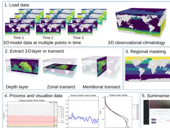
In this section, we describe the five-stage evaluation process that the toolkit applies to model and observational data. Fig-ure 1 summarises the evaluation process graphically. 3.1 Load model and observational data
The first stage of the evaluation process is to load the model and observational data. The model data are typically a time series of two- or three-dimensional variables stored in one or several NetCDF files. Please note that we use the standard convention of only counting spatial dimensions. As such, any mention of dimensionality here implies an additional tempo-ral dimension; i.e. three-dimensional model data have length, height, width, and time dimensions.
The model data can be a single NetCDF variable or some combination of several variables. For instance, in some ma-rine biogeochemistry models, total chlorophyll concentra-tion is calculated as the sum of many individual phytoplank-ton functional type chlorophyll concentrations. In all cases, BGC-val loads the model data one time step at the time, whether the NetCDFs contain one or multiple time steps.
The front-loading evaluation functions described in Sects. 2.3 and 4.3.1 are applied to each time step of the model data at this point. The resulting loaded data can be a one-, two-, or three-dimensional array. The use of an observational dataset is optional, but allows the model to be compared against historical measurements. The observational data and model data are not required to be loaded using the same func-tion.
When loading data, BGC-val assumes that we use the NetCDF format. The NetCDF files are opened in BGC-val with a custom Python interface,dataset.py, in the
bgcvaltoolspackage. The datasetclass is based on
Figure 1.The five stages of the evaluation process. The first stage is the loading of the model and observational data. The second stage is the extraction of a two-dimensional array. The third stage is regional masking. The fourth stage is processing and visualisation of the data. The fifth stage is the publication of an html summary report. Note that the three figures shown in the fourth stage are repeated below in Figs. 3, 4, and 6.
3.2 Extract a two-dimensional slice
The second evaluation stage is the extraction of a two-dimensional variable from three-two-dimensional data. As shown in the second panel of Fig. 1, the two-dimensional variable can be the surface of the ocean, a depth layer parallel to the surface, an east–west transect parallel to the Equator, or a north–south transect perpendicular to the Equator. This stage is included in order to speed up the process of evaluating a model; in general, it is much quicker to evaluate a 2-D field than a 3-D field. Furthermore, the spatial and transect maps produced by the evaluation process can become visually con-fusing when overlaying several layers. Note that stages 2 and 3 are applied to both model and observational data (if present). This stage is unnecessary if the data loaded in the first stage are already a two-dimensional variable, such as the fractional sea ice coverage, or a one-dimensional variable, such as the Drake Passage Current.
In the case of a transect, instead of extracting along the file’s internal grid, the transect is produced according to the geographic coordinates of the grid. This is done by locating points along the transect line inside the grid cells based on the grid cell corners.
3.3 Extract a specific region
Stage 3 is the masking of specific regions or depth lev-els from the 2-D extracted layer, as described in Sect. 2.4. Stage 3 is not needed if the variable is already a one-dimensional product, such as the total global flux of CO2. Stage 3 takes the two-dimensional slice, then converts the data into five one-dimensional arrays of equal length. These arrays represent the time, depth, latitude, longitude, and value of each data point in the data. These five 1-D arrays can be further reduced by making cuts based on any of the coordinates or even cutting according to the data.
Both stages 2 and 3 of the evaluation process reduce the number of grid cells under evaluation. This two-stage pro-cess is needed because the stage 3 masking cut can become memory intensive. As such, it is best to for the data to ar-rive at this stage in a reduced format. In contrast, the stage 2 process of producing a 2-D slice is a relatively computation-ally cheap process. This means that the overall evaluation of a model run can be done much faster.
3.4 Produce visualisations
data, a simple time series, and the time development of the depth profile. However, several other visualisations can also be produced: for instance, the point-to-point comparisons of model data against observational data and a comparison of the same measurement between different regions, times or models, or scenarios.
Which visualisations are produced depends on which eval-uation switches are turned on, but also a range of other fac-tors including the dimensionality of the model dataset and the presence of an observational dataset. For instance, figures that show the time development of the depth profile require three-dimensional data. Similarly, the point-to-point compar-ison requires an observational dataset for the model to match against. More details on the range of plotting tools are avail-able in Sects. 4.2.1 and 4.2.2.
Stages 1–4 are repeated for each evaluated field and for multiple models scenarios or different versions of the same model. If multiple jobs or models are requested, then com-parison figures can also be created in stage 4.
3.5 Produce a summary report
The fifth stage is the automated generation of a summary re-port. This is an html document which shows the figures that were produced as part of stages 1–4. This document is built from html and can be hosted and shared on a web server. More details on the report are available in Sect. 4.2.3.
4 Code structure and functionality
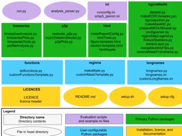
The directory structure of the BGC-val toolkit repository is summarised in Fig. 2. This figure highlights a handful of the key features. We use the standard Python nomen-clature where applicable. In Python, a module is a Python source file, which can expose classes, functions, and global variables. A package is simply a directory containing one or more modules and Python creates a package using the
__init__.py file. The BGC-val toolkit contains seven packages and dozens of modules.
In this figure, ovals are used to show single files in the head directory, and rectangles show folders or packages. In the top row of Fig. 2, there are two purple ovals and a rectangle which represent the important evaluation scripts and the example configuration files. These files include the
run.py executable script, which is a user-friendly wrap-per for theanalysis_parser.pyscript (also in the head directory). Theanalysis_parser.pyfile is the princi-pal Python file that loads the run configuration and launches the individual analyses. Theinidirectory includes several example configuration files, including the configuration files that were used to produce the figure in this document. Note that theinidirectory is not a Python package, just a repos-itory that holds several files. A full description of the func-tionality of configuration files can be found in Sect. 4.1.
The four main Python packages in BGC-val are shown in green rectangles in Fig. 2. Each of these modules has a specific purpose: the timeseries package described in Sect. 4.2.1 performs the evaluation of the time development of the model, thep2ppackage described in Sect. 4.2.2 does an in-depth spatial comparison of a single point in time for the model against a historical data field, and thehtml pack-age described in Sect. 4.2.3 contains all the Python functions and html templates needed to produce the html summary re-port. Thisbgcvaltools package contains many Python routines that perform a range of important functions in the toolkit. These tools include, but are not limited to, a tool to read NetCDF files, a tool to extract a specific 2-D layer or transect, a tool to read and understand the configuration file, and many others.
The three user-configurable packages functions,
regions, andlongnamesare shown in blue in Fig. 2. The
functionspackage, described in Sect. 4.3.1, contains all the front-loading analysis functions described in Sect. 2.3, which are applied in the first stage of the evaluation pro-cess described in Sect. 3. Theregionspackage described in Sect. 4.3.2 contains all the masking tools described in Sect. 2.4 and which are applied in the third stage of the evaluation process described in Sect. 3. Thelongnames
package, described in Sect. 4.3.3, is a simple tool which be-haves like a look-up dictionary, allowing users to link human-readable or “pretty” names (like “chlorophyll”) against the internal code names or shorthand (like “chl”). The pretty names are used in several places, notably in the figure titles and legends and on the html report.
The licences directory, the setup configuration files and the README.md are all in the main directory of the folder, as shown in yellow in Fig. 2. The licences directory contains information about the Revised Berkeley Software Distribution (BSD) three-clause licence. TheREADME.md
file contains specific details on how to install, set up, and run the code. Thesetup.pyandsetup.cfgfiles are used to install the BGC-val toolkit.
4.1 The configuration file
The configuration file is central to the running of BGC-val and contains all the details needed to evaluate a simulation. This includes the file path of the input model files, the user’s choice of analysis regions, layers, and functions, the names of the dimensions in the model and observational files, the final output paths, and many other settings. All settings and configuration choices are recorded in an single file using the
.iniformat. Several example configuration files can also be found in theinidirectory. Each BGC-val configuration file is composed of three parts: an active keys section, a list of evaluation sections, and a global section. Each of these parts is described below.
The tools that parse the configuration file are in the
pack-<number>
html
makeReportConfig.py htmlTools.py figure-template.html section-template.html
htmlAssets p2p
testsuite_p2p.py matchDataAndModel.py
p2pPlots.py ... timeseries
timeseriesAnalysis.py timeseriesPlots.py
timeseriesTools.py profileAnalysis.py
...
bgcvaltools
dataset.py makeEORCAmasks.pyc
bgcvalpython.py makeMaskNC.py prepareMEDUSAyear.py
configparser.py regionMapLegend.py
RobustStatistics.py extractLayer.py mergeMonthlyFiles.py removeMaskFromshelve.py
Primary Python packages
functions stdfunctions.py customFunctionsTemplate.py
…
regions makeMask.py customMaskTemplate.py
...
longnames longnames.py longnames.ini customLongNames.ini
User-configurable Python packages
LICENCES
LICENCE licence header
Directory name Directory contents
README.md setup.sh setup.cfg
Evaluation scripts and example ini files
Installation, licence, and documentation
File in head directory
ini
runconfig.ini cmip5_jasmin.ini analysis_parser.py
Legend run.py
Figure 2.The structure of the BGC-val repository. The principal directories are shown as rectangles, with the name of the directory in bold followed by the key files contained in that directory. Individual files in the head directory are shown with rounded corners. The evaluation scripts and the configuration directory are shown in purple. The primary Python modules are split into four directories, shown in green rectangles. The three user-configurable Python modules are shown as blue rectangles. The licence, README, and setup files are shown in yellow.
age. These tools interpret the configuration file and use them to direct the evaluation. Please note that we use the standard
.ini format nomenclature while describing configuration files. In this,[Sections]are denoted with square brack-ets, each option is separated from its value by a colon, “:”, and the semi-colon “;” is the comment syntax in.ini for-mat.
4.1.1 Active keys section
The active keys section should be the first section of any BGC-val configuration file. This section consists solely of a list of Boolean switches, one Boolean for each field that the user wants to evaluate.
[ActiveKeys]
Chlorophyll : True
A : False
; B : True
To reiterate the ini nomenclature, in this example
ActiveKeysis the section name, andChlorophyll,A, andBare options. The values associated with these options are the BooleansTrue,False, andTrue. OptionBis com-mented out and will be ignored by BGC-val.
In the[ActiveKeys]section, only options whose val-ues are set to True are active. False Boolean values and commented lines are not evaluated by BGC-val. In this ex-ample, theChlorophyllevaluation is active, but both op-tionsAandBare switched off.
4.1.2 Individual evaluation sections
EachTrueBoolean option in the[ActiveKeys]section needs an associated [Section] with the same name as the option in the[ActiveKeys]section. The following is an example of an evaluation section for chlorophyll in the HadGEM2-ES model.
[Chlorophyll]
name : Chlorophyll
units : mg C/m^3
; The model name and paths
model : HadGEM2-ES
modelFiles : /Path/*.nc
modelgrid : CMIP5-HadGEM2-ES
; Model coordinates/dimension names
model_t : time
model_cal : auto
model_z : lev
model_lat : lat
model_lon : lon
; Data and conversion
model_vars : chl
model_convert : multiplyBy
model_convert_factor : 1e6
dimensions : 3
; Layers and Regions
layers : Surface 100m
regions : Global SouthernOcean
Thenameandunitsoptions are descriptive only; they are shown on the figures and in the html report, but do not influence the calculations. This is set up so that the name as-sociated with the analysis may be different to the name of the fields being loaded. Similarly, while NetCDF files often have units associated with each field, they may not match the units after the user has applied an evaluation function. For this reason, the final units after any transformation must be supplied by the user. In the example shown here, HadGEM2-ES correctly used the CMIP5 standard units for chlorophyll concentration, kg m−3. However, we prefer to view chloro-phyll in units of mg m−3.
The modeloption is typically set in the Global sec-tion, described below in Sect. 4.1.3, but it can be set here as well. The modelFiles option is the path that BGC-val should use to locate the model data files on local stor-age. The modelFilesoption can point directly at a sin-gle NetCDF file or can point to many files using wild cards (*, ?). The file finder uses the standard Python package
glob, so wild cards must be compatible with that pack-age. Additional nuances can be added to the file path parser using the placeholders $MODEL, $SCENARIO, $JOBID,
$NAME, and$USERNAME. These placeholders are replaced with the appropriate global setting as they are read by the
configparserpackage. The global settings are described below in Sect. 4.1.3. For instance, if the configuration file is set to iterate over several models, then the$MODEL place-holder will be replaced by the model name currently being evaluated.
ThegridFileoption allows BGC-val to locate the grid description file. The grid description file is a crucial require-ment for BGC-val, as it provides important data about the model mask, the grid cell area, and the grid cell volume. Minimally, the grid file should be a NetCDF which contains the following information about the model grid: the cell-centred coordinates for longitude, latitude, and depth, and these fields should use the same coordinate system as the field currently being evaluated. In addition, the land mask
should be recorded in the grid description NetCDF in a field calledtmask, the cell area should be in a field called
area, and the cell volume should be recorded in a field labelled pvol. BGC-val includes the meshgridmaker
module in the bgcvaltools package and the function
makeGridFilefrom that module can be used to produce a grid file. Themeshgridmakermodule can also be used to calculate the cross-sectional area of an ocean transect, which is used in several flux metrics such as the Drake Passage Cur-rent or the Atlantic meridional overturning circulation.
Certain models use more than one grid to describe the ocean; for instance, NEMO uses a U grid, a V grid, a W grid, and a T grid. In that case, care needs to be taken to ensure that the grid file provided matches the data. The name of the grid can be set with themodelgridoption.
The names of the coordinate fields in the NetCDF need to be provided here. They aremodel_t for the time and
model_calfor the model calendar. Any NetCDF calen-dar option (360_day, 365_day, stancalen-dard, Gregorian, etc.) is also available using the model_caloption; however, the code will preferentially use the calendar included in standard NetCDF files. For more details, see thenum2datefunction of thenetCDF4Python package (https://unidata.github.io/ netcdf4-python/, last access: 5 October 2018). The depth, lat-itude, and longitude field names are passed to BGC-val via themodel_z,model_lat, andmodel_lonoptions.
The model_vars option tells BGC-val the names of
the model fields that we are interested in. In this example, the CMIP5 HadGEM2-ES chlorophyll field is stored in the NetCDF under the field namechl. As already mentioned, HadGEM2-ES used the CMIP5 standard units for chloro-phyll concentration, kg m−3, but we prefer to view chloro-phyll in units of mg m−3. As such, we load the chlorophyll field using the conversion functionmultiplyByand give it the argument 1e6 with themodel_convert_factor
option. More details are available below in Sect. 4.3.1 and in theREADME.mdfile.
BGC-val uses the coordinates provided here to extract the layers requested in the layers option from the data loaded by the function in the model_convert option. In this example that would be the surface and the 100 m depth layer. For the time series and profile analyses, the layer slicing is applied in the DataLoader class in
the timeseriesTools module of the timeseries
package. For the point-to-point analyses, the layer slic-ing is applied in thematchDataAndModel class in the
matchDataAndModelmodule of thep2ppackage.
Once the 2-D field has been extracted, BGC-val masks the data outside the regions requested in theregionsoption. In this example, that is theGlobaland theSouthernOcean
regions. These two regions are defined in the regions
package in themakeMaskmodule. This process is described below in Sect. 4.3.2.
it is masked or sliced. The dimensionality of the loaded vari-able affects how the final results are plotted. For instance, one-dimensional variables such as the global total primary production or the total Northern Hemisphere ice extent can-not be plotted with a depth profile or with a spatial compo-nent. Similarly, two-dimensional variables such as the air– sea flux of CO2or the mixed layer depth should not be plot-ted as a depth profile, but can be plotplot-ted with percentile dis-tributions. Three-dimensional variables such as the tempera-ture and salinity fields, the nutrient concentrations, and the biogeochemical advected tracers are plotted with time se-ries, depth profile, and percentile distributions. If any spe-cific types of plots are possible but not wanted, they can be switched off using one of the following options.
makeTS : True
makeProfiles : False
makeP2P : True
The makeTS option controls the time series plots, the
makeProfiles option controls the profile plots, and the makeP2Poption controls the point-to-point evaluation plots. These options can be set for each active keys section, or they can be set in the global section, as described below.
In the case of the HadGEM2-ES chlorophyll section, shown in this example, the absence of an observational data file means that some evaluation figures will have blank areas, and others figures will not be made at all. For instance, it is impossible to produce a point-to-point comparison plot with-out both model and observational data files. The evaluation of [Chlorophyll]could be expanded by mirroring the model’s coordinate and convert fields with a similar set of data coordinates and convert functions for an observational dataset.
4.1.3 Global section
The[Global]section of the configuration file can be used to set default behaviour which is common to many evaluation sections. This is because the evaluation sections of the con-figuration file often use the same option and values in sev-eral sections. As an example, the names that a model uses for its coordinates are typically the same between fields; i.e. a chlorophyll data file will use the same name for the lati-tude coordinate as the nitrate data file from the same model. Setting default analysis settings in the [Global] section ensures that they do not have to be repeated in each evalua-tion secevalua-tion. As an example, the following is a small part of a global settings section.
[Global]
model : ModelName
model_lat : Latitude
These values are now the defaults, and individual evalua-tion secevalua-tions of this configuraevalua-tion file no longer require the
model or model_latoptions. However, note that local
settings override the global settings. Note that certain options such asnameorunitscannot be set to a default value.
The global section also includes some options that are not present in the individual field sections. For instance, each configuration file can only produce a single output report, so all the configuration details regarding the html report are kept in the global section.
[Global]
makeComp : True
makeReport : True
reportdir : reports/HadGEM2-ES_chl
The makeComp is a Boolean flag to turn on the
comparison of multiple jobs, models, or scenarios. The
makeReportis a Boolean flag which turns on the global report making andreportdiris the path for the html re-port.
The global options jobID, year, model, and
scenario can be set to a single value or can be set to multiple values (separated by a space character) by swap-ping them with the options jobIDs, years, models, or scenarios. For instance, if multiple models were requested, then swap
[Global]
model : ModelName1
with the following.
[Global]
models : ModelName1 ModelName2
For the sake of the clarity of the final report, we recom-mend only setting one of these options with multiple val-ues at one time. The comparison reports are clearest when grouped according to a single setting; i.e. please do not try to compare too many different models, scenarios, and job IDs at the same time.
The [Global] section also holds the paths to the lo-cation on disc where the processed data files and the out-put images are to be saved. The images are saved to the paths set with the following global options: images_ts,
images_pro,images_p2p, andimages_compfor the
time series, profiles, point-to-point, and comparison fig-ures, respectively. Similarly, the post-processed data files are saved to the paths set with the following global options:
postproc_ts, postproc_pro, andpostproc_p2p
for the time series, profiles, and point-to-point-processed data files, respectively.
As described above, the global fields jobID, year,
model, andscenariocan be used as placeholders in file paths. Following the bash shell grammar, the placeholders are marked as all capitals with a leading $ sign. For instance, the output directory for the time series images could be set to the following.
[Global]
$MODELand$NAMEare placeholders for the model name string and the name of the field being evaluated. In the ex-ample in Sect. 4.1.2 above, theimages_tspath would
be-comeimages/HadGEM2-ES/Chlorophyll. Similarly,
the basedir_modelandbasedir_obsglobal options
can be used to fill the placeholders$BASEDIR_MODELand
$BASEDIR_OBSsuch that the base directory for models or observational data does not need to be repeated in every sec-tion.
A full list of the contents of a global section can be found in theREADME.mdfile. Also, several example configuration files are available in theinidirectory.
4.2 Primary Python packages
In this section, we describe the important packages that are shown in green in Fig. 2. The timeseries package is described in Sect. 4.2.1, the p2p package is described in Sect. 4.2.2, and thehtmlpackage is described in Sect. 4.2.3. All the figures in Sect. 4.2 were produced on the JASMIN computational resource using the example configuration file
ini/HadGEM2-ES_no3_cmip5_jasmin.ini, and
the html summary report associated with that configuration file is available in the Supplement.
Outside the three main packages described below, the
bgcvaltoolspackage contains many Python routines that perform a range of important functions. These tools include a tool to read NetCDF files dataset.py, a tool to ex-tract a specific 2-D layer or transectextractLayer.py, and a tool to read and understand the configuration file,
configparser.py. There is a wide and diverse selection of tools in this directory: some of them are used regularly by the toolkit, and some are only used in specific circumstances. More details are available in theREADME.mdfile, and each individual module in thebgcvaltoolsis sufficiently doc-umented that its role in the toolkit is clear.
4.2.1 Time series tools
Thistimeseriespackage is a set of Python tools that pro-duces figures showing the time development of the model. These tools manage the extraction of data from NetCDF files, the calculation of a range of metrics or indices, the storing and loading of processed data, and the production of figures illustrating these metrics.
Firstly, the time development of any combination of depth layer and region can be investigated with these tools. The spatial regions can be taken from the predefined list or a cus-tom region can be created. The predefined regions are listed in the regions directory of the BGC-val. Many metrics are available including, mean, median, minimum, maximum, and all percentiles divisible by 10 (10th percentile, 20th per-centile, etc.). Furthermore, any user-defined custom function can also be included as a custom function, for instance the
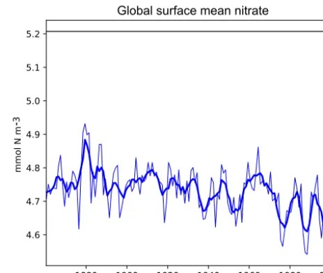
Figure 3.A plot produced by the time series package. This fig-ure shows the time development of a single metric, in this case the global surface mean nitrate in HadGEM2-ES in the historical simu-lation. It also shows the 5-year moving average of the metric.
calculation of global total integrated primary production or the total flux through the Drake Passage.
The time series tools produce three types of analysis plots. Examples of these three types of figures are shown in Figs. 3, 4, and 5. All three examples use annual averages of the nitrate (CMIP5 name: no3) in the surface layer of the global ocean in the HadGEM2-ES model historical scenario, ensemble member r1i1p1.
Figure 3 shows the time development of a single vari-able: the mean of the nitrate in the surface layer over the entire global ocean. This figure shows the annual mean of the HadGEM2-ES model’s nitrate as a thin blue line, the 5-year moving average of the HadGEM2-ES model’s nitrate as a thick blue line, and the World Ocean Atlas (WOA) data (Garcia et al., 2013b) as a flat black line. The WOA data used here are an annual average climatological dataset and hence do not have a time component. This figure highlights the fact that the model simulates a decrease in the mean surface ni-trate over the course of the 20th century.
Figure 4.A plot produced by the time series package. The figure shows the time developers of many metrics at once: the mean, median, and several percentile ranges of the observational data and the model data. In this case, the model data are the global surface mean nitrate in HadGEM2-ES in the historical simulation.
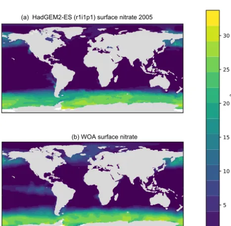
Figure 5.A plot produced by the time series package. The figure shows the spatial distribution of the model(a)and the observational dataset(b). In this case, the model data are the global surface mean nitrate in HadGEM2-ES in the historical simulation.
percentile figures can be produced for any layer and spatial region and these metrics are all area weighted. For all three kinds of time series figures, a real dataset can be added, al-though it is not possible to include the time development of the observational dataset at this stage.
The time series package also produces a figure showing the spatial distribution of the model and observational data. Figure 5 shows an example of such a figure, in which panel (a) shows the spatial distribution of the final time step of the model, and panel (b) shows the spatial distribution of the
ob-servational dataset. It is possible to plot data for any layer for any region. These spatial distributions are made using the Plate Carré projection, and the projections are set to focus on the region in question. Figure 5 highlights the fact that the HadGEM2-ES model failed to capture the high nitrate seen in the observational data in the equatorial Pacific.
BGC-val can also produce several figures showing the time development of the model datasets over their en-tire water columns. The profile modules are stored in the
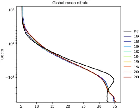
timeseriespackage, as the time series and profiles fig-ures share many of the same underlying methods. Figfig-ures 6, 7, and 8 are examples of three profile plots showing the time development over the water column of the global mean ni-trate in the HadGEM2-ES model historical simulation, en-semble member r1i1p1. These plots can only be produced when the data have three dimensions. These plots can be made for any region from the predefined list or for custom regions.
Figure 6 shows the time development of the depth profile of the model and observational data. Thex axis shows the value, in this case the nitrate concentration in mmol N m−3 and they axis shows depths. These types of plots always show the first and last time slice of the model, then a subset of the other years is also shown. Each year is assigned a dif-ferent colour, with the colour scale shown in the right-hand side legend. If available, the observational data are shown as a black line. This figure shows the annual mean of the World Ocean Atlas nitrate climatology dataset as a black line.
Figure 6.The time development of the global mean dissolved ni-trate over a range of depths. This figure shows the HadGEM2-ES global mean nitrate over the entire water column; each model year is included as a coloured line, and the annual mean of the World Ocean Atlas nitrate climatology dataset is shown as a black line.
the entire water column in the year 1880. This does not ap-pear to be a fault in the model, but simply a brief period dur-ing which the difference was slightly larger than zero. This peak in the mean is also visible in the global mean surface ni-trate in Fig. 3, but is not visible in the percentile distribution of the surface nitrate in Fig. 4.
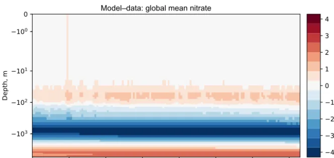
Figures 6, 7, and 8 all show that the model data match the observational nitrate near the surface, but diverge at depth. The model underestimates the peak in the global mean of the observational nitrate at a depth of approximately 1000 m and then overestimates the observed nitrate below 2000 m. Also, the model does not show much interannual variability in the structure of the global annual average nitrate over the 145-year simulation. However, it is unclear from the WOA annual average whether we should expect any variability from the model over this time range.
In thetimeseriespackage, there is also a set of tools for comparing the time series development between multiple versions of the same metric. This is effectively the same as plotting several versions of Fig. 3 on the same axes. This kind of diagram can be useful to compare the same measurement between different regions, depth layers, or different members of a model’s ensemble. However, these plots can also be used to compare multiple models. Several example figures are in-cluded in Sect. 5.
4.2.2 Point-to-point model–data comparison tools In addition to the time series evaluation, BGC-val can per-form a direct point-to-point comparison of model against data. The point-to-point tools here are based on the work by de Mora et al. (2013). In that work, we demonstrated that
using point-to-point analysis is more representative of a real marine dataset than comparing the bulk mean of the model to the bulk mean of the data. The method involves matching the model data to the closest corresponding observational mea-surement, then hiding all model points which do not have a corresponding observational measurement and vice versa. The point-to-point methodology means that the model and observational data have not be re-interpolated to a common grid: they both retain their original grid description.
Figures 9, 10, and 11 show examples of the figures made by the point-to-point package. In all three figures, the model data are the global surface nitrate in HadGEM2-ES in the historical simulation in ensemble member r1i1p1 in the year 2000. The observational data come from the nitrate dataset in the World Ocean Atlas (Garcia et al., 2013b).
Figure 9 is a group of four spatial distributions compar-ing the model and observational datasets. The map in Fig. 9a is the model, Fig. 9b is the observations, Fig. 9c is the dif-ference between the model and observations (model minus observational data), and Fig. 9d is the quotient (model over observational data). This example shows the comparison at the ocean surface, but these tools also allow for longitudi-nal or latitudilongitudi-nal transect comparisons or a spatial distribu-tion along a specific depth level. This figure shows that the year 2000 of the HadGEM2-ES model reproduces the large-scale spatial patterns seen in the observational dataset. The model has significantly higher nitrate that the observational climatology in the Southern Ocean, the North Pacific, and the equatorial regions and has significantly lower nitrate in the Arctic regions. A discrepancy in the spatial extent of the high nitrate in the Southern Ocean is shown clearly in the dif-ference panel of this figure. The quotient panel of this figure also shows that model underestimates the low-nitrate regions around the tropical waters.
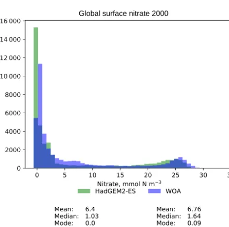
Figure 10 is a pair of histograms showing the same model and observational data as in Fig. 9. This figure also shows some measures of the central tendency (mean, median, mode) and measures of the deviation (standard deviation and median absolute deviation) for both model and data. These histograms confirm that the model underestimates the nitrate concentration in the low-nitrate region, which covers a sig-nificant region and is the mode of the WOA dataset.
Global mean nitrate
Figure 7.The time development of the global mean dissolved nitrate over a range of depths. The figure shows the same data as Fig. 6, but as a Hovmöller time series plot. The annual mean of the World Ocean Atlas nitrate climatology dataset is shown as a column on the right-hand side of the figure.
Figure 8.The time development of the global mean dissolved nitrate over a range of depths. The figure shows the same data as Figs. 6 and 7, but with the World Ocean Atlas nitrate observational measurement subtracted from the model time series.
more than half of the nitrate observations between 10 and 20 mmol N m−3.
4.2.3 HTML report
The html package of the BGC-val toolkit contains all the tools needed to produce a report summarising the output of the time series, the profile, and the point-to-point packages. The principal file in this package is the
makeReportConfig module, which produces an html
document according to the settings of the configuration file. Using the configuration file, the report maker finds all the im-ages and uses several template files to stitch together the indi-vidual sections of the report. The html is based on a template taken from https://html5up.net/ (last access: 5 October 2018), used under the Creative Commons Attribution 3.0 License.
An example of the HTML report is avail-able in the Supplement. This report shows
the output of the example configuration file:
ini/HadGEM2-ES_no3_cmip5_jasmin.ini. In
order to access this report, please download and unzip the files, then export them to a local copy before opening the
index.htmlfile in a browser of your choice. 4.3 User-configurable Python packages
In this section, we look at the code behind the extensive cus-tomisability of BGC-val: thefunctions,regions, and
longnamespackages shown in blue in Fig. 2 are described in this section. The functions package is described in Sect. 4.3.1, theregionspackage is described in Sect. 4.3.2, and thelongnamespackage is described in Sect. 4.3.3. 4.3.1 Functions
Figure 9.Four spatial distributions showing the model(a), the observational data(b), the difference between them(c), and their quotient(d). The model data in these plots are the global surface nitrate in HadGEM2-ES in the historical simulation in ensemble member r1i1p1 in the year 2000. The observational data come from the annual nitrate dataset in the World Ocean Atlas.
Global surface nitrate 2000
Figure 10.A pair of histograms showing the model (green) and the observational data (blue), as well as some metrics of the distribution shape. The model data are the global surface nitrate in HadGEM2-ES in the historical simulation in the year 2000. The observational data come from the nitrate dataset in the World Ocean Atlas. The metrics are the mean, median, the mode, the standard deviation,σ, and the median absolute deviation (MAD).
applied to a dataset as the data are loaded. In most cases, the conversion is one of the standard functions such as multiply or divide by some arbitrary number, add a constant value to the variable, or simply just load the data as is with no con-version. However, this package can also be used to perform complex data processing.
Figure 11.This figure shows the distribution of the model and the observational data with the model data along thex axis and the observation data along theyaxis. The model data are the global surface nitrate in HadGEM2-ES in the historical simulation in the year 2000. The observational data come from the nitrate dataset in the World Ocean Atlas. The 1:1 line is shown as a dashed line. A linear regression is shown as a full line, with the slope, intersect,P value, correlation, and number of data points shown on the right-hand side.
Thedata_convertandmodel_convertoptions in
the configuration file allow BGC-val to determine which function to apply to the model or observational data as they are loaded. There is no default function, so to simply load the data into the file, the standard functionNoChangeshould be specified in thedata_convertormodel_convert op-tions.
As an example of the structure of a basic function, we look at a simplified version of themultiplyByfunction in the
def multiplyBy(nc,keys, **kwargs): f = float(kwargs[’factor’])
return nc.variables[keys[0]][:]*f
After declaring the function name and arguments in the first line, this function loads thefactorfrom the keyword arguments (kwargs) and parses it into the single precision floating format in the second line. In the third line, this func-tion loads the first item in thekeyslist from the NetCDF datasetnc, then multiplies that data by the factorf, and re-turns the product. The path to the NetCDF file, the choice of function, the list of keys, and the factor are all provided by the configuration file.
All functions need to be called with the same arguments:
ncis a NetCDF file opened by thedatasetmodule from thebgcvaltoolspackage. Thekeysargument is a list of strings which represent the names of fields in a NetCDF file, and the optionalkwargsargument is used to pass any extra information that is needed (such as a factor or addend).
The keyword arguments which are passed to the func-tion must be preceded by the text model_convert_or
data_convert_ strings in the configuration file. In the example above, the “factor” was written in the configuration file as
model_convert_factor : 1e6
but it was loaded in the multiplyBy function as
kwargs[’factor’].
Some evaluation metrics require multiple variables to be loaded at once and combined together. The
stdfunctionsmodule of thefunctionspackage
con-tains a few such medium-complexity operations, such as “sum”, which returns the sum of the fields in thekeyslist. The’divide’function returns the quotient of the first key over the second key from thekeyslist.
More complex functions can be implemented as well, for instance depth integration, global totals, or the flux through a certain cross section. There are several examples of com-plex functions in the functions folder. Note that some of these functions can change the dimensionality of the data, and cau-tion needs to be taken to ensure that thedimensions op-tion in the configuraop-tion file matches the dimensions of the output of this function.
4.3.2 Regions
Similarly to the functions package described above, the re-gions package allows for expanded flexibility in the evalua-tion of models. The term “region” here is a portmanteau for any selection of data based on their coordinates or values. Typically, these are spatial regional cuts, such as “Northern Hemisphere”, but the masking is not limited to spatial re-gions. For instance, theregionspackage can also be used to remove negative values and to remove zero,NaN, orinf
values.
As an example of the structure of a basic regional mask, we look at the SouthHemisphere region in the
makeMaskmodule of theregionspackage.
def SouthHemisphere( name,region, xt,xz,xy,xx,xd):
a = np.ma.masked_where(xy>0.,xd) return a.mask
The Python standard packageNumPyhas been imported asnp. Each regional masking function has access to the fol-lowing fields: name, the name of the data; region, the name of the regional cut; xt, a one-dimensional array of the dataset times;xz, a one-dimensional array of the dataset depths;xy, a one-dimensional array of the dataset latitudes;
xx, a one-dimensional array of the dataset longitudes; and
xd, a one-dimensional array of the data. The second to last line creates a masked array of the data array which is masked in all the places where the latitude coordinate is greater than zero (i.e. the Northern Hemisphere). The final line returns the mask for this array. All region extraction functions return a NumPy mask array. In Python, NumPy masks are an array of Booleans in which “true” is masked.
Many regions are already defined in the file
regions/makeMask.py, but it is
straightfor-ward to add a new region using the template
file regions/customMaskTemplate.py.
To do this, make a copy of the
regions/customMaskTemplate.py file in the
regions directory, rename the function and file to your mask name, and add whatever cuts are required. BGC-val will be able to locate your region, provided that the region name matches the Python function and the region in your configuration file.
4.3.3 Long names
In the Python source code, objects are often abbreviated or labelled with shorthand, and spaces and hyphens are not acceptable in object names. This means that the internal name of a model, dataset, field, layer, or region is not usu-ally the same in the text that we want to appear in public plots. For this reason, the long name package has a dictio-nary of common terms with their abbreviated name linked to a “pretty” name. The dictionary has definitions for each model, scenario, dataset, object, mask, cut, region, field, and other pythonic object used in BGC-val. These pretty names are used when preparing outwards-facing graphics and html pages such that the name of an object in the configuration file is not a source of confusion.
no3 : Nitrate
chl : Chlorophyll
This means that we can label nitrate internally as “no3” as the evaluation name in our configuration file, but when it appears in plots, it will be shown as “nitrate”. Also note that the options are not case sensitive, but the values are case sensitive. While the default long name list is already rela-tively extensive, users can add their own long names to the
longnames/customLongNames.inifile.
5 Applying BGC-val to CMIP5 RCP8.5
In this section, we show some example figures of the inter-comparison of several CMIP5 models. These examples were produced using CMIP5 data on the JASMIN data process-ing facility (http://www.jasmin.ac.uk, last access: 5 Octo-ber 2018), and the configuration file used to produce these is supplied in the BGC-val Git repository under the name
cmip5_rcp85_jasmin.ini in the inidirectory. The
examples that we show here are the Atlantic meridional overturning circulation in Fig. 12, the Antarctic circumpo-lar current in Fig. 13, the total annual air to sea flux of CO2 in Fig. 14, the total annual marine primary production in Fig. 15, and the global mean surface chlorophyll in Fig. 16. All five figures here show the 5-year moving average instead of the monthly or annual time resolution of the field in or-der to improve clarity. The 5-year window moving average is calculated using the mean of 2.5 years on either side of a central point. This means that the start and end points of the time series are the mean of only 2.5 years.
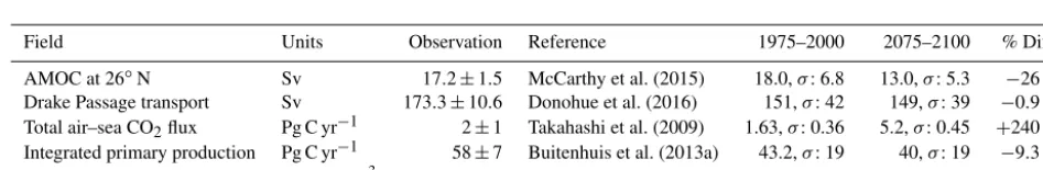
Table 1 shows the observational measurement for the multi-model mean of the years 1975–2000 in the historical scenario, the multi-model mean of the years 2075–2100 un-der the RCP8.5 scenario, and the percentage of change be-tween 2075–2100 and 1975–2000 for all five fields.
These examples compare a subset of the CMIP5 mod-els in the historical time range and RCP8.5 scenario in the ensemble member r1i1p1. The historical and RCP8.5 simulations are aligned such that the historical simulation links to the RCP scenario at the year 2005. This was done using the jasmin_cmip5_linking.py module in the
bgcvaltoolspackage.
The CMIP5 models shown in these figures are CESM1-BGC, CMCC-CESM, GFDL-ESM2G, GFDL-ESM2M, GISS-E2-H-CC, GISS-E2-R-CC, HadGEM2-CC, HadGEM2-ES, IPSL-CM5A-MR, IPSL-CM5B-LR, MPI-ESM-LR, MPI-ESM-MR, and NorESM1-ME. This report does not include all CMIP5 models, but rather a small number of examples of marine circulation and biogeochem-istry metrics over the historical and RCP8.5 scenarios. The selection criterion was that the model was required to have biogeochemical datasets in the British Atmospheric Data Centre (BADC) archive of the CMIP5 data. The BADC is a UK mirror of the CMIP5 data archive, which is managed by
the Centre for Environmental Data Analysis (CEDA), and this archive is accessible from the JASMIN data processing facility. We also required the r1i1p1 job identifier and the “latest” model run tag.
Using these tools, we uncovered a previously undetected error in the HadGEM2-ES RCP8.5 r1i1p1 simulation. The HadGEM2-ES RC8.5 r1i1pi simulation contains 2 years in which the annual mean data were produced without all 12 months. This made the two erroneous years differ sig-nificantly from the other years in our time series plots. Af-ter informing the HadGEM2-ES project manager, we were advised to substitute the r2i1p1 simulation in place of the HadGEM2-ES r1i1p1 simulation.
The Atlantic meridional overturning circulation (AMOC) is a major current and consists of two parts: a northbound transport between the surface and approximately 1200 m and a southbound transport between approximately 1200 and 3000 m (Kuhlbrodt et al., 2007). The AMOC is responsi-ble for the production of roughly half of the ocean’s deep waters (Broecker, 1991). The northward heat transport of the AMOC is substantial and has a significant role in the climate of the Northern Hemisphere. The strength of the northbound AMOC in several CMIP5 models was shown in Fig. 12.35 of the IPCC report (Collins et al., 2013). The BGC-val toolkit was able to reproduce the AMOC analy-ses of the IPCC. As in the IPCC figure, Fig. 12 shows the historical and RCP8.5 projections of the AMOC produced by BGC-val. Please note that we use a different subset of CMIP5 models in this figure relative to IPCC Fig. 12.35. The RAPID array measured the long-term mean of the AMOC to be 17.2±1.5 Sv between 2004 and 2013 (McCarthy et al., 2015). This figure is shown as a black rectangle with a grey background in Fig. 12. The calculation was initially based on the methods used in the UK Met Office’s internal ocean evaluation toolkit, Marine Assess, which uses the calcula-tion described in Kuhlbrodt et al. (2007) and McCarthy et al. (2015). However, we have since expanded the original Ma-rine Assess method to be model and grid independent. This cross-sectional area for the 26◦N transect was calculated and saved to a NetCDF file using the meshgridmaker
module in thebgcvaltoolspackage. The model-specific cross-sectional area was used to calculate the maximum of the depth-integrated cross-sectional current in the custom functioncmip5AMOCin thecirculationmodule in the
functionspackage. Amongst the CMIP5 models that in-cluded a biogeochemical component, several models overes-timated the AMOC, and several underesoveres-timated the AMOC in the historical simulation. However, nearly all simulations predict a decline in the AMOC over the 21st century, and the multi-model mean drops by 26 % from 18 Sv in the mean of the years 1975–2000 to 13 Sv in the mean of the years 2075– 2100 under the RCP8.5 scenario.
Figure 12.The Atlantic meridional overturning circulation at 26◦N in a subset of CMIP5 models. Each model is shown as a full line, and the historical measurement is shown as a grey area. The model data are a 5-year moving average.
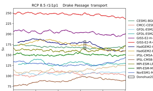
Figure 13.The Drake Passage Current. Each model is shown as a full line, and the historical measurement is shown as a grey area. The model data are a 5-year moving average.
around Antarctica and is the dominant feature of the circu-lation of the Southern Ocean. The ACC was recently mea-sured through the Drake Passage at 173.3±10.7 Sv (Dono-hue et al., 2016), making the ACC the strongest ocean cur-rent in the world. A metric to describe the ACC is the to-tal volume transport through the narrow gap between South America and Antarctica, known as the Drake Passage, shown in Fig. 13. Here, the Drake Passage Current is calculated as the total depth-integrated current between the South Amer-ican coast and the Antarctic peninsula along a line of con-stant longitude at 78◦W. To perform this calculation in a grid-independent way, a north–south line was drawn along
Figure 14.The total annual flux of CO2from the air to the sea in Pg yr−1under the RCP8.5 scenario
Figure 15.The total annual marine primary production of a range of models.
using themeshgridmakermodule in thebgcvaltools
package. The calculation was performed in the custom
func-tion cmip5DrakePassagein the circulation
mod-ule in the functionspackage. Figure 13 shows a mov-ing average with a 5-year window for several CMIP5 mod-els between the years 1860 and 2100 in units of Sver-drups and the observation of 173.3±10.7 Sv from Donohue et al. (2016). Several CMIP5 models make estimates of the Drake Passage transport within the uncertainty of the obser-vational measurement. The percentage of difference between the multi-model means of 1975–2000 and 2075–2100 under the RCP8.5 scenario is a decrease of 0.9 %, even though the inter-model spread is particularly large (70–250 Sv).
The ocean is a major sink of CO2and absorbed approxi-mately 27 % of anthropogenic CO2emissions between 2002 and 2011 (Le Quéré et al., 2013). The total air–sea flux of CO2from the atmosphere to the ocean is an important metric for understanding the fate of greenhouse gases (Takahashi et al., 1997). The total global air to sea flux of CO2 from various CMIP5 models is shown in Fig. 14 and the obser-vational range of 2±1 Pg C yr−1for the year 2000 is taken from Takahashi et al. (2009). Note that the observational data were recorded between 1970 and 2007, but scaled to the year 2000. The calculation was performed in the custom function
TotalAirSeaFluxCO2 in theAirSeaFluxCO2