The Thirty-Third AAAI Conference on Artificial Intelligence (AAAI-19)
A Two-Stream Mutual Attention Network for
Semi-Supervised Biomedical Segmentation with Noisy Labels
Shaobo Min, Xuejin Chen,
∗Zheng-Jun Zha, Feng Wu, Yongdong Zhang
National Engineering Laboratory for Brain-inspired Intelligence Technology and Application, University of Science and Technology of China, Hefei, Anhui, China
Abstract
Learning-based methods suffer from a deficiency of clean an-notations, especially in biomedical segmentation. Although many semi-supervised methods have been proposed to pro-vide extra training data, automatically generated labels are usually too noisy to retrain models effectively. In this paper, we propose a Two-Stream Mutual Attention Network (TS-MAN) that weakens the influence of back-propagated gra-dients caused by incorrect labels, thereby rendering the net-work robust to unclean data. The proposed TSMAN consists of two sub-networks that are connected by three types of attention models in different layers. The target of each at-tention model is to indicate potentially incorrect gradients in a certain layer for both sub-networks by analyzing their inferred features using the same input. In order to achieve this purpose, the attention models are designed based on the propagation analysis of noisy gradients at different layers. This allows the attention models to effectively discover in-correct labels and weaken their influence during parameter updating process. By exchanging multi-level features within two-stream architecture, the effects of noisy labels in each sub-network are reduced by decreasing the noisy gradients. Furthermore, a hierarchical distillation is developed to pro-vide reliable pseudo labels for unlabelded data, which further boosts the performance of TSMAN. The experiments using both HVSMR 2016 and BRATS 2015 benchmarks demon-strate that our semi-supervised learning framework surpasses the state-of-the-art fully-supervised results.
Introduction
Recently, many successful deep networks have been pro-posed to segment 3D magnetic resonance (MR) data (Tseng et al. 2017; C¸ ic¸ek et al. 2016; Yu et al. 2017a; 2017b). How-ever, the scarcity of clean, labeled data severely hinders fur-ther development of deep learning methods for real applica-tions. Even for manual annotation, it is inevitable that data experts may make mistakes due to the effects of fatigue and human error. Thus, it is urgently important to improve the robustness of networks to noisy labels and generate more reliable machine annotations. In this paper, we design a net-work that is less disturbed by noisy labels and propose a
∗
Corresponding Author.
Copyright c2019, Association for the Advancement of Artificial Intelligence (www.aaai.org). All rights reserved.
Labeled Data
Manual Labels
Unlabeled Data
Pseudo Labels
Data with Noisy Labels
Two-Stream Mutual
Attention Network
Hierar
ch
ical
Distillatio
n
Figure 1: The pipeline of our self-training framework. The hierarchical distillation first generates reliable pseudo labels for unlabeled data, and then mixed data is used to retrain the two-stream mutual attention network, which is robust to noisy labels.
simple but effective distillation model to generate reliable pseudo labels.
Self-training is a typical semi-supervised method, which generates pseudo labels for unlabeled data by using trained models. Obviously, the quality of pseudo labels is crucial to the performance of a final retrained model. Among ex-isting methods that generate labels automatically, model distillation (Hansen and Salamon 1990; Gupta, Hoffman, and Malik 2016) is one of the most widely used methods, which aggregates the inferences from multiple models for better pseudo labels. Different from model distillation,
Ra-dosavovicet al.(2018) recently proposed a data distillation
that aggregates the inferences from multiple transformations of a data sample; this method proves to be superior to model distillation. Although both distillation methods are effective, the generated pseudo labels are still noisy, which limits the performance of self-training.
sam-ples with same wrong predictions can effectively prevent in-correct updates, because annotations for hard samples are more likely to be noisy. This inference procedure using pre-diction disagreement is useful for discovering noisy updates caused by incorrect labels; however, Malach and Shalev-Shwartz (2017) ignore that the intermediate information dur-ing generatdur-ing prediction is also important.
In this paper, we propose a two-stream mutual attention network (TSMAN) by comprehensively exchanging multi-level features between two networks in different layers, in-cluding their predictions. To give an example, our intuition tells us that if two students share a teacher, it is impor-tant to analyze the nature of these students mistakes to de-termine whether the errors are unique or result from in-structional gaps. Based on this intuition, we use attention models in multiple layers to discover potential incorrect la-bels and weaken the corresponding gradients during back-propagation. A vital challenge is how to provide useful clues about noisy gradients for attention models to infer noise dis-tribution. To address this issue, a two-stream architecture is developed by connecting two sub-networks with multi-attention models, which collect information from two sub-networks to discover noisy gradients. By analyzing the noisy label propagation process, three kinds of attention models are designed for different layer depths, which successfully weakens the noisy gradients propagated by the loss layer. By weakening the noisy gradients in multiple layers, our TSMAN is robust to noisy labels in biomedical data and performs comparably to fully-supervised learning methods when only partial annotations are used.
Furthermore, a hierarchical distillation method is pro-posed to combine data distillation (Radosavovic et al. 2018) and model distillation (Hansen and Salamon 1990). With the high quality of pseudo labels generated by our hierarchi-cal distillation, the performance of TSMAN in self-training tasks can be further improved.
The whole self-training process of our method is shown in Figure 1. The overall contributions are summarized as fol-lows:
• We propose a novel two-stream mutual attention network
(TSMAN), that is robust to noisy labels, and it can be ex-tended to many applications, when clean annotations are difficult to acquire.
• The proposed hierarchical distillation is more effective
than either data or model distillation in generating reliable pseudo labels.
• The proposed self-training framework with TSMAN and
hierarchical distillation is superior to existing methods for biomedical segmentation.
Related Work
In this section, we briefly discuss two categories of related work: networks that are robust to noisy labels and self-training methods that use distillation.
In supervised learning models, the topic of improved re-silience to noisy labels has been widely studied. Barandela and Gasca (2000) remove the labels that are suspected to
be incorrect before retraining. Inspired by the minimum en-tropy regularization in (Grandvalet and Bengio 2004), Reed et al. (2014) propose adding a regularization term, which is related to the current prediction, to the network’s loss function. Mnih and Hinton (2012) use a probabilistic model to calculate the probability of each label being incorrect, and avoid updating in case incorrect labels occur.
McDow-ellet al.(2007) propose novel generalizations for three
com-parison algorithms that examine how cautiously or aggres-sively each algorithm exploits noisy intermediate relational data. Goldberger and Ben-Reuven (2017) apply the Expecta-tion MaximizaExpecta-tion (EM) algorithm by iteratively estimating true labels and retraining the network, which requires two-phase training to optimize two distinct softmax layers. Re-cently, Malach and Shalev-Shwartz (2017) tackle this prob-lem by training two predictors with different initializations and only updating when there is a disagreement between
their predictions. Han et al. (2018) present an effective
co-teaching learning paradigm by simultaneously training two models and removing noisy samples from each mini-batch of data, which is conceptually similar to our method. However, in our method for segmentation, each sample has densely arranged labels, which is different from the form of classification in (Han et al. 2018). Thus, exploring the spatial relationship among labels helps us learn from noisy labels in the segmentation stage; this significant step is of-ten ignored in existing methods. Based on the recently suc-cess of attention mechanism (He et al. 2018; Yue et al. 2018; Zhang et al. 2017; Chen et al. 2018), we use the multiple at-tention models between layer pairs in two simultaneously trained networks to weaken noisy gradients. This process not only considers the prediction disagreement but also ex-changes the evidence during inference.
The self-training approach is the earliest for semi-supervised learning, and it uses the predictions of a model on unlabeled data to retrain itself for better perfor-mance. Without using post-processing, many distillation ap-proaches have been widely adopted for self-training. Gupta
et al. (2016) propose the cross model distillation for
tack-ling the problem of limited labels. Laine and Aila (2016) ag-gregate the inferences of multiple checkpoints during train-ing to avoid traintrain-ing multiple models. Besides model dis-tillation, data distillation is also an effective method to ex-plore new information from data transformations. Simon
et al. (2017) obtain extra data from different views to
re-train models, which yields an excellent performance in hand
keypoint detection. Moreover, Radosavovic et al. (2018)
demonstrate that an inference to multiple transformations of a data point is superior to any of the predictions under a sin-gle transform. Inspired by the above methods, we propose combining data distillations and model distillations in a hi-erarchical way to incorporate the unique advantages of both model and data distillation.
Two-Stream Mutual Attention Network
BN+ReLU+Conv. Loss Layer Data Flow DenseBlock Pooling Deconv.+ReLu
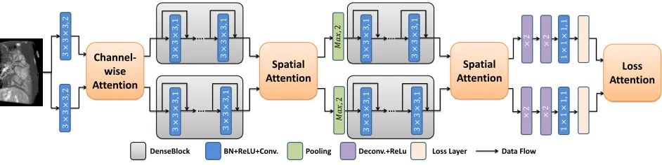
3 × 3 × 3 ,2 × 2 × 2 1 × 1 × 1 ,1 3 × 3 × 3 ,2 … 3 × 3 × 3 ,1 … 3 × 3 × 3 ,1 Channel-wise Attention Spatial Attention 3 × 3 × 3 ,1 Spatial Attention × 2 1 × 1 × 1 ,1 3 × 3 × 3 ,1 𝑀𝑎𝑥 ,2 𝑀𝑎 𝑥 ,2 3 × 3 × 3 ,1 3 × 3 × 3 ,1 Loss Attention × 2 … 3 × 3 × 3 ,1 … 3 × 3 × 3 ,1 3 × 3 × 3 ,1 3 × 3 × 3 ,1 𝑀𝑎 𝑥 ,2
Figure 2: The diagram of TSMAN. For readability, we present the parameters of Conv, pooling, and Deconv layers on the
operation units. Each DenseBlock consists of12BN+ReLU+Conv units.
Problem Formulation
We denotexas an input data sample withN elements and
˜
yas the observed labels, possibly with some noise. For
ex-ample, in a binary segmentation task,xcan be a 2D array
withN pixels, andy˜ = {±1}N is the label array
indicat-ing which class each pixel belongs to. Our goal is to train a
model on{x,y˜}that is comparable to{x,y}, wherey is
the clean label array. For simplicity, we denotey={±1}N.
Then, y˜ can be written asy˜ = θ.∗y, where .∗ denotes
element-wise multiplication of two arrays. For most pixels
whose labels are correct,θi = 1.θi =−1indicates that the
label is wrong for pixeli.
Without losing generalization, a fully convolutional
net-work is trained on {x,ye}, in which the weights updating
layerdare represented by:
∂Ls(p,θ.∗y)
∂wd =
∂Ls(p,θ.∗y) ∂od
∂od
∂wd, (1)
∂Ls(p,θ.∗y)
∂od =
∂Ls(p,θ.∗y) ∂od+1
∂od+1
∂od , (2)
whereodis the output features of layerd,wdis the
convo-lutional weights,Ls is the objective function, andpis the
prediction of the network. Therefore, the target is to weaken
the gradients fromyiwithθi=−1in Eq. (1) and Eq. (2).
To this end, an intuitive way is to obtain an attention modelfatt, and then:
∂Ls(p,θ.∗y)
∂p ⇒
∂Ls(p,θ.∗y)
∂p fatt(p,h). (3)
Ideally, whenθi =−1,fatt(pi,h)is expected to be0with
the extra information h. Next, we will introduce how to
provide useful extra informationhto indicate the potential
noisy gradients in the network.
Two-Stream Architecture
We believe that the inference processing of another net-work is helpful to discover incorrect updates in this netnet-work. Thus, we train two networks with the same inputs and use
the predictionspbfrom the other network ashin Eq. (3):
∂Ls(p,θ.∗y)
∂od ⇒
∂Ls(p,θ.∗y)
∂od f
k
att(p,pb). (4)
However, as the information in pb is unable to indicate
all wrong gradients in ∂Ls(p,θy)
∂od , some noisy gradients will
be propagated to previous layers. To this end, multiple fattk (od,hd)are applied in different layers to weaken noisy
gradients in the whole network as much as possible by:
∂Ls(p,θ.∗y)
∂od ⇒
∂Ls(p,θ.∗y)
∂od f
k att(o
d,
b
od). (5)
Our two-stream mutual attention network is thus designed as a symmetric two-stream architecture, as shown in Figure 2. The four attention models take in both feature maps from two sub-networks and give two feedback attention maps to indicate their potential wrong gradients. Notably, three types of attention models are used: loss attention (LA), spatial at-tention (SA), and channel-wise atat-tention (CA). These atten-tion models will be introduced in detail in the following sec-tion.
Finally, the loss of TSMAN is:
L=Ls(p,θ.∗y) +Ls(p,b θ.∗y). (6)
The final prediction for a test sample is obtained by averag-ing the softmax outputs of two networks.
Loss Attention
In our task, a reasonable hypothesis is that the same pre-dictions from two sub-networks usually occur when the input sample is extremely simple or hard. The extremely simple samples are easy to predict correctly by both sub-networks, which means that the loss can be ignored in back-propagation for model fine-tuning. The extremely hard sam-ples are more likely to be annotated falsely, which means that their labels are unreliable and can also be ignored in back-propagation. Based on this hypothesis, the loss atten-tion model (LA) is designed to remove these two kinds of samples by:
fatt4 (p,pb) =ω(p⊕pb) (7)
where⊕is the pixel-wise exclusive OR operations, andωis
the weights of a Gaussian smoothing convolution operation that is applied to(p⊕pb).
It should be noted that singlep⊕pbserves as a binary loss selector. Although checking disagreements between
(a) Image (b) Attention (c) Smoothing
Figure 3: The black pixels in (b) indicate that the predictions of two sub-networks for (a) are different. (c) is obtained by applying Gaussian smoothing to (b), which corresponds to Eq. (7). After smoothing, more voxels in the input image (a) are involved for back-propagation to improve the networks.
b
pi, it ignores a special case whenpi,pbi are both wrong but
e
yi is correct. In this special case, the correct labels are
use-ful but ignored in back-propagation by only usingp⊕pb.
To this end, we introduce ω to alleviate this problem. We
observe that the disagreements of pi andpbi usually occur
on the boundaries (black voxels in Figure 3 (b)). The voxels near these boundaries are challenging for sub-networks, but they are relatively easier for experts to annotate. This means
that an xi that is near boundaries is more likely to have
both wrong pi,pbi and a correct eyi. Therefore, we employ
a smoothing operation on the attention map to partially pre-serve the pixels near boundaries during back-propagation; the attention map for this is shown in Figure 3 (c). After
smoothing,fatt4 in Eq. (7) becomes non-binary.
Spatial and Channel-wise Attention
Since loss attention only extracts information from the final predictions of two sub-networks, we also exploit the mutual information from middle feature maps of two models. Two types of attention models are introduced: spatial attention model and channel-wise attention model.
By definingod
i ∈RCas the feature vector ati-th position
on the feature maps of layerd, whereCis the feature map
channel, we know that the shallow layers receive more noisy gradients than deep layers, due to the larger receptive field on ∂Ls(p,θ.∗y)
∂od . In other word, ifdis small, it is more likely
forodi to receive a noisy gradient. Based on these
observa-tions, we use a spatial attention (SA) model asf3
att, since it
is close to the loss layer and few gradients ofodi are noisy.
The spatial attention map is expected to weaken the noisy gradients in a small number of regions, which is efficient and feasible to implement. Forfatt1,2, the attention models are too far from the loss layer, which means that the propagated
gradient for almost allod
i have been polluted by incorrect
labels. Therefore, the spatial attention becomes inappropri-ate because the gradients of all feature vectors are noisy and should be weakened, which leads to a slow convergence. To this end, the channel-wise attention (CA) is used forfatt1,2to select useful feature channels. Both SA and CA serve as fea-ture selectors during inference, as well as gradient selectors during back-propagation. Figure 4 gives the detailed imple-mentations of both SA and CA.
𝑀3× 𝐶
43× 𝐶
43× 𝐶
13× 𝐶
max pooling
𝑀3× 𝐶
max pooling conv (1 × 1 × 1) conv (1 × 1 × 1)
43× 𝐶
+
43× 𝐶 conv (4 × 4 × 4) conv (4 × 4 × 4)1-sigmoid(∙) 1-sigmoid(∙)
13× 𝐶
(b) Channel-wise attention
Input1 Input2
Output1 Output2
conv (1 × 1 × 1)
Input1
𝑀3× 𝐶 𝑀3× 𝐶
conv (1 × 1 × 1)
𝑀3× 𝐶
+
𝑀3× 𝐶Output1 Output2
conv (1 × 1 × 1) conv (1 × 1 × 1)
ReLu
(a) Spatial attention
1-sigmoid(∙) 1-sigmoid(∙)
𝑀3× 1 𝑀3× 1
Input2
Figure 4: The spatial attention (a) and channel-wise attention (b) diagrams. The blue circles indicate the element-wise ad-ditions, and the parameters in the convolution block indicate
the kernel sizes. M,C respectively represent the size and
channel of the feature map.
Hierarchical Distillation
While the proposed TSMAN provides an effective training strategy when there is noise in labels, a hierarchical
distilla-tion method is also proposed to reduce noisy labels (yeiwith
negative θi) in pseudo labels. Our hierarchical distillation
method integrates data distillation and model distillation
to-gether. We defineLas the labeled data space,Uas the
unla-beled data space, andfas the well-trained model onL. The
model distillation and data distillation respectively produce
pseudo labels forU by:
PM D(I) = g {ft(I)|t= 1,· · · , T}
(8)
PDD(I) = g¯h−1k (f(¯hk(I)))|k= 1,· · ·, K
(9)
whereI∈ Uand¯hkare thek-th transformation forI, which
include rotation and flipping, while¯h−1k is the
correspond-ing inverse transformation.g({·})is the voting function. It is important to note that data distillation aggregates inferences
ofK transformations of input data, which proves to be
su-perior for model distillation. However, this requires enough
labeled data to train a suitablef. Model distillation is more
robust when the labeled data is insufficient, as it explores
complementary information fromT models.
Both model and data distillation methods are effective in improving the reliability of pseudo labels for self-training, but they distill knowledge from different views. Therefore, we combine them in a hierarchical way to take advantage of both of them:
PHD = g {PtDD(I)|t= 1,· · · , T}
(10)
wherePtDD is the data distillation operation usingft. The
Experiments
In this section, several ablation studies are first given to prove the effectiveness of the proposed method, and then comparisons with brand-new methods are introduced on HVSMR 2016 challenges (Pace et al. 2015) and BRATS 2015 (Kistler et al. 2013) benchmarks.
Datasets
The HVSMR 2016 dataset consists of10 3D cardiac MR
scans for training and10 scans for testing. The resolution
of each scan is about200×140×120. All the MR data is
scanned from patients with congenital heart disease (CHD), which is hard to diagnose. The annotations contain the my-ocardium and blood pool regions in cardiac MR images. The testing results are submitted to a public platform and evalu-ated by the organizer. To alleviate the problem of overfit-ting, we apply data augmentations, including random rota-tions and flipping.
The training set for the BRATS-2015 dataset consists of 220 subjects with high-grade gliomas and 54 subjects with low-grade gliomas. The resolution of each MRI image is
155×240×240. The platform for BRATS-2015 requires
dis-guised evaluation, and most methods have fully-supervised training without published experimental settings. Thus we follow (Tseng et al. 2017) by using 195 high-grade gliomas and 49 low-grade gliomas in the training set, and the re-maining 30 subjects for evaluation. There are five labels that correspond to common issues: edema, non-enhancing core, necrotic core, and enhanced core regions.
Evaluation Metrics
For HVSMR 2016, we use the overall score (higher is better) provided by the official platform for ablation analysis as our evaluation metric. In comparison with recent methods from HVSMR 2016, we report three main metrics from the plat-form, including the mean Dices (a higher value is better), the average distance of boundaries, and the Hausdorff distance (lower values are better). For BRATS-2015, we report the mean Dices criterion for all the five labels.
Implementation Details
We employ the DenseVoxNet (Yu et al. 2017a) as the sub-network in our two-stream architecture. The training param-eters, as well as the data pre-processing, follow the settings in (Yu et al. 2017a), except for the max iterations, which are
35,000due to the disturbance of noisy labels.
For hierarchical distillation,12geometric transformations
are applied to each data point, including combinations of four rotations and three flips. Three models, with different
initializations and max iterations (10000,15000and20000),
are used for the ensemble.
In order to evaluate the robustness of experimental meth-ods to noisy labels, the training datasets are divided into two parts. The first part uses the manual labels, and the second part uses the pseudo labels from hierarchical distillation. The
proportions of manual labels are controlled byξto imitate
different situations of noisy labels.
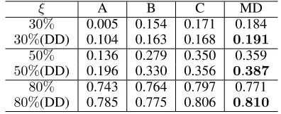
Table 1: Comparison of overall scores of different
distilla-tion methods on HVSMR 2016.ξ is set to be30%,50%,
and80%.DDindicates the data distillation, and MD is the
model distillation. A, B, and C are three base models to be aggregated for distillation.
ξ A B C MD
30% 0.005 0.154 0.171 0.184
30%(DD) 0.104 0.163 0.168 0.191
50% 0.136 0.279 0.350 0.359
50%(DD) 0.196 0.330 0.356 0.387
80% 0.743 0.764 0.797 0.771
80%(DD) 0.785 0.775 0.806 0.810
Table 2: Effects of different attention models. The baseline
is our TSMAN without anyfatt.
f1
att fatt2 fatt3 fatt4 score
Baseline -1.167
TSMAN
√
-0.737
√ √
-0.601
√ √ √
-0.576
√ √ √ √
−0.561
Evaluation of Hierarchical Distillation.
In this part, we compare our hierarchical distillation with data distillation (Radosavovic et al. 2018) and model dis-tillation (Hansen and Salamon 1990) under different set-tings. The implementations of data and model distillation are special cases of hierarchical distillation that use a sin-gle model or no geometric transformation. In Table 1, we report the performance of the above methods when we split
the HVSMR dataset withξ= 30%,50%, and80%.
From Table 1, it can be observed that both data and model distillations are effective in improving the quality of pseudo
labels. However, when ξ = 30%, model distillation
per-forms better than data distillation according to the overall
scores 0.184and0.168(highest among three base models
with data distillation), respectively. The opposite case is true whenξ= 80%. A possible reason for this is that the perfor-mance of multi-transformation inferences relies on the abil-ity of its base model. When the base model is trained with
insufficient labels (30%), the data distillation improvement
is weak or even negative, as in the case of model C. How-ever, model distillation is less dependent on a certain model, as it distills knowledge from multiple models. Therefore, it can be concluded that data distillation is more effective when base models are well-trained with plenty of correct la-bels, while model distillation is more robust to insufficient clean labels. Both advantages of data and model distilla-tion are crucial due to the various situadistilla-tions of biomedical datasets. Therefore, our hierarchical distillation is a more general method as it takes advantage of both model and data distillations.
(a) (b) (c) (d) (e) 𝒌 = 𝟒
𝒌 = 𝟑
𝒊𝒕𝒆𝒓 = 𝟐𝟓𝒌 𝒊𝒕𝒆𝒓 = 𝟐𝟓𝒌
𝒊𝒕𝒆𝒓 = 𝟏𝟓𝒌 𝒊𝒕𝒆𝒓 = 𝟏𝟓𝒌
𝒌 = 𝟒 𝒌 = 𝟑
Figure 5: Two sections of 3D MRI data. The labels in col-orful regions in (b), (c) are wrong, and the gradients in the
yellow regions are weakened byf3
attandfatt4 , respectively.
Notably, the more yellow, the smaller the response in the at-tention map. (d) and (e) are the predictions before and after retraining using unlabeled data. The red regions are the my-ocardium, the green regions are blood pools, and the yellow regions are incorrect predictions. After retraining, the area of yellow regions becomes smaller.
Analysis of the TSMAN
In order to demonstrate the effectiveness of the TSMAN’s design, we first explore the effects of different attention models in TSMAN. As noisy gradients are propagated from deep to shallow layers, we report the results by
sequen-tially applying attention models from fatt4 to fatt1 in
Ta-ble 2. From the information in TaTa-ble 2, adding afk
att(k =
1,2,3,4) each time obviously improves the performance,
which means that allfatt1,2,3,4effectively weaken noisy
gra-dients in their corresponding layers. Besides, we find that
the improvement offattk is usually weaker thanf
k+1
att . The
reason is that noisy gradients in shallow layers are harder to discover, and some noisy gradients have been weakened by the latter attention model.
Next, some visual examples of spatial attentions are
shown in Figure 5 (b) and (c) to prove the effects offatt3
andf4
att in weakening noisy gradients. From Figure 5 (b)
and (c), we observe that partial noisy gradients, marked in yellow, have been correctly eliminated by attention models, which proves the effectiveness of multiple attention models.
Especially forf4
att, we also explore the effects of smoothing
operations in Eq. 7, and an 0.1 score improvement is
ob-tained by usingωwith a kernel size of3×3and a variance
of0.5. Finally, after retraining, the segmentation of TSMAN
is obviously better, as shown in Figure 5 (d) and (e).
Comparisons Using the HVSMR 2016 Dataset
In order evaluate the robustness of our method to different unclean datasets, we compare the TSMAN with state-of-the-art methods (Malach and Shalev-Shwartz 2017; Tang et al. 2017; Yu et al. 2017a) by splitting the HVSMR 2016
dataset with ξ = 10%,· · · ,90%. (Malach and
Shalev-Shwartz 2017) is implemented by training two networks and assigning a non-zero loss weight for a voxel when their
pre-0 0.1 0.2 0.3 0.4 0.5 0.6 0.7 0.8 0.9 1
ξ
-4 -3.5 -3 -2.5 -2 -1.5 -1 -0.5 0 0.5
overall score
-3.185 -1.498
-1.224
-1.167 -1.053 -0.748
-1.027 -0.404
-3.250 -1.298
-1.321
-1.067 -1.053 -0.978
-0.937 -0.451
-2.740
-0.964 -0.859
-0.742 -0.464 -0.415 -0.416 -0.272
-2.319
-0.760 -0.612 -0.561
-0.348 -0.315 -0.256 -0.024 [Yu et al., 2017] (fully supervised)
[Yu et al., 2017] [Jagersand,2017]
[Malach and Shalev-Shwartz, 2017] TSMAN
Figure 6: Evaluations of different methods on HVSMR 2016
dataset with different ξ. The overall scores are calculated
using the testing data.
dictions are different. For a fair comparison, we train two models for the other methods, and the predictions are av-eraged for the final results. The results are shown in Fig-ure 6. As illustrated, when the labeled data is insufficient
(ξ ∈ [10%,20%]), the performances of all the
learning-based methods are unsatisfactory. This is because the quality of pseudo-labels is insufficient for providing useful
informa-tion for model retraining. Whenξincreases, noise decreases
in pseudo-labels and models begin to learn extra knowledge from the unlabeled data. Then, the performance of our TS-MAN and (Malach and Shalev-Shwartz 2017) is better than (Tang et al. 2017) and the baseline. The reason is that stu-dent models learn more from fewer noisy labels, thus they have more consistent opinions during learning, which filters out many noisy labels. Note that our TSMAN is better than (Malach and Shalev-Shwartz 2017), as shown in Figure 6, which demonstrates that the exchange of multi-level features is better than only the predictions. Finally, whenξ= 0.9, our retrained model even surpasses the fully-supervised model, which proves that there is also noise in the manual labels.
Next, we compare our TSMAN (usingξ= 0.9) with the
Table 3: Comparison of different approaches using the HVSMR 2016 dataset. To save space, we use the first ini-tial of the first author’s last name combined with the last two digits of the year to indicate the methods, which respectively refer to [Mukhopadhyay, 2016], [Tziritas, 2016], [Van Der Geest, 2017], [Wolterink et al., 2016], [Yu et al., 2016] and [Yu et al., 2017] from top to bottom.
Myocardium Blood Pool Overall Dice ADB HDD Dice ADB HDD Scores M16 0.495 2.596 12.8 0.794 2.550 14.6 NA T16 0.612 2.041 13.2 0.867 2.157 19.7 -1.408 V17 0.747 1.099 5.09 0.885 1.553 9.41 -0.330 W16 0.802 0.957 6.13 0.926 0.885 7.07 -0.036 Y16 0.786 0.997 6.42 0.931 0.868 7.01 -0.055 Y17 0.821 0.960 7.29 0.931 0.938 9.53 -0.161 Ours 0.820 0.824 4.73 0.926 0.957 8.81 −0.024
0 0.1 0.2 0.3 0.4 0.5 0.6 0.7 0.8 0.9 1
ξ
0.2 0.3 0.4 0.5 0.6 0.7 0.8
mean Dice
0.392 0.571
0.643 0.672
0.685 0.691
0.700
0.338 0.585
0.650 0.658
0.689 0.687
0.708
0.421 0.618
0.683 0.701
0.716 0.721 0.738
0.458 0.652
0.707
0.729 0.746
0.755 0.762 MME
[Yu et al., 2017] [Jagersand,2017]
[Malach and Shalev-Shwartz, 2017] TSMAN
Figure 7: Evaluations of different methods on BRATS 2015
with differentξ. The mean Dice of five labels are reported in
the validation set.
Comparisons using the BRATS 2015 dataset
We further evaluate our method on a larger 3D MRI dataset, the Brats 2015 benchmark, to prove its effectiveness. Us-ing experiments similar to those with the HVSMR 2016 dataset, we compare TSMAN with (Malach and Shalev-Shwartz 2017), (Tang et al. 2017), MME (Tseng et al. 2017)
and baseline DVN(Yu et al. 2017a) with differentξ. Notably,
we use the public results of MME and 3D U-net in (Tseng et al. 2017) that use one-phase training, and the mean IOU for five labels are reported.
Figure 7 gives evaluations of different methods using the
BRATS 2015 dataset with differentξ. From the results, it
is apparent that the performance of TSMAN and (Malach and Shalev-Shwartz 2017) are better than (Tang et al. 2017) and baseline DenseVoxNet. This further proves that improv-ing robustness to noisy labels obviously benefits the semi-supervised learning performance. Especially since Tseng
et al.(Tseng et al. 2017) only provide the results of
fully-supervised models without codes available, we use this as
a fully supervised baseline. Finally, whenξ = 0.9, our
re-trained model also surpasses the fully-supervised (Tseng et
Table 4: Comparison of recent approaches on the BRATS 2015 dataset.
Label 0 1 2 3 4 mean
U-Net 0.923 0.429 0.736 0.453 0.620 0.632 MME 0.966 0.943 0.712 0.328 0.960 0.782 DVN 0.989 0.426 0.730 0.645 0.850 0.728 TSMAN 0.990 0.7760 0.720 0.684 0.790 0.792
al. 2017).
In Table 4, we compare our TSMAN model (ξ = 0.9)
with U-Net (Ronneberger, Fischer, and Brox 2015), MME (Tseng et al. 2017), and DVN (Yu et al. 2017a), which are fully-supervised and trained. This also demonstrates that TSMAN is robust to noisy labels.
Conclusion
In this paper, we propose a two-stream mutual attention network (TSMAN) that is robust to noisy labels. This net-work discovers incorrect labels and weakens the influence of these incorrect labels during the parameter updating process. Specifically, three kinds of attention models are designed to connect multiple layers of two sub-networks; the attention models analyze the layers’ features and indicate potential noisy gradients. To improve the quality of pseudo labels, our hierarchical distillation takes advantage of both data and model distillations by hierarchically combining these two methods. Finally, combining TSMAN and hierarchical dis-tillation in a self-training manner leads to state-of-the-art performance on the HVSMR 2016 and Brats 2015 bench-marks.
In the future, we hope that only one sub-network will be sufficient for completing inferences during testing. This may be achieved by generating attention maps and apply-ing them to gradients of feature maps durapply-ing the trainapply-ing process. Also, we will explore the effects of using different sub-networks, which may increase the challenge of design-ing attention models.
Acknowledgement
This work was supported by the National Natural Sci-ence Foundation of China under Nos. 61472377, 61632006, 91732304, and 61525206, the Fundamental Research Funds for the Central Universities under Grant WK2380000002, the National Key Research and Development Program of China (2017YFC0820600), National Defense Science and Technology Fund for Distinguished Young Scholars (2017-JCJQ-ZQ-022).
References
Barandela, R., and Gasca, E. 2000. Decontamination of training samples for supervised pattern recognition
meth-ods. InJoint IAPR International Workshops on Statistical
Techniques in Pattern Recognition (SPR) and Structural and
Chen, X.; Liu, D.; Zha, Z.-J.; Zhou, W.; Xiong, Z.; and Li, Y. 2018. Temporal hierarchical attention at category-and
item-level for micro-video click-through prediction. In2018 ACM
Multimedia Conference on Multimedia Conference, 1146–
1153. ACM.
C¸ ic¸ek, ¨O.; Abdulkadir, A.; Lienkamp, S. S.; Brox, T.; and
Ronneberger, O. 2016. 3D u-net: learning dense
volumet-ric segmentation from sparse annotation. In International
Conference on Medical Image Computing and
Computer-Assisted Intervention, 424–432.
Goldberger, J., and Ben-Reuven, E. 2017. Training deep
neural-networks using a noise adaptation layer. In
Interna-tional Conference on Learning Representations (ICLR).
Grandvalet, Y., and Bengio, Y. 2004. Semi-supervised
learn-ing by entropy minimization. InAdvances in neural
infor-mation processing systems (NIPS), 529536.
Gupta, S.; Hoffman, J.; and Malik, J. 2016. Cross modal
distillation for supervision transfer. InThe IEEE
Confer-ence on Computer Vision and Pattern Recognition (CVPR),
2827–2836.
Han, B.; Yao, Q.; Yu, X.; Niu, G.; Xu, M.; Hu, W.; Tsang, I.; and Sugiyama, M. 2018. Co-teaching: robust training deep
neural networks with extremely noisy labels.arXiv preprint
arXiv:1804.06872.
Hansen, L. K., and Salamon, P. 1990. Neural network
en-sembles. IEEE transactions on pattern analysis and
ma-chine intelligence12(10):993–1001.
He, A.; Luo, C.; Tian, X.; and Zeng, W. 2018. A twofold
siamese network for real-time object tracking. InThe IEEE
Conference on Computer Vision and Pattern Recognition
(CVPR), 4834–4843.
Kistler, M.; Bonaretti, S.; Pfahrer, M.; Niklaus, R.; and B¨uchler, P. 2013. The virtual skeleton database: an open access repository for biomedical research and collaboration.
Journal of medical Internet research15(11).
Laine, S., and Aila, T. 2016. Temporal ensembling for
semi-supervised learning. InInternational Conference on
Learn-ing Representations (ICLR).
Malach, E., and Shalev-Shwartz, S. 2017. Decoupling
”when to update” from ”how to update”. InAdvances in
Neural Information Processing Systems. 961971.
McDowell, L. K.; Gupta, K. M.; and Aha, D. W. 2007.
Cau-tious inference in collective classification. InAAAI
Confer-ence on Artificial IntelligConfer-ence, 596–601.
Mnih, V., and Hinton, G. E. 2012. Learning to label aerial
images from noisy data. InProceedings of the 29th
Interna-tional conference on machine learning (ICML), 567–574.
Pace, D. F.; Dalca, A. V.; Geva, T.; Powell, A. J.; Moghari,
M. H.; and Golland, P. 2015. Interactive whole-heart
segmentation in congenital heart disease. InInternational
Conference on Medical Image Computing and
Computer-Assisted Intervention, 8088.
Radosavovic, I.; Dollr, P.; Girshick, R.; Gkioxari, G.; and He, K. 2018. Data distillation: Towards omni-supervised
learning. InThe IEEE Conference on Computer Vision and
Pattern Recognition (CVPR), 4119–4128.
Reed, S.; Lee, H.; Anguelov, D.; Szegedy, C.; Erhan, D.; and Rabinovich, A. 2014. Training deep neural networks on
noisy labels with bootstrapping. InProceedings of the 29th
International conference on machine learning (ICML).
Ronneberger, O.; Fischer, P.; and Brox, T. 2015. U-net: Convolutional networks for biomedical image segmentation.
In International Conference on Medical image computing
and computer-assisted intervention, 234–241. Springer.
Simon, T.; Joo, H.; Matthews, I.; and Sheikh, Y. 2017. Hand keypoint detection in single images using multiview
boot-strapping. InThe IEEE Conference on Computer Vision and
Pattern Recognition (CVPR), 1145–1153.
Tang, M.; Valipour, S.; Zhang, Z.; Cobzas, D.; and Jager-sand, M. 2017. A deep level set method for image
segmenta-tion. InDeep Learning in Medical Image Analysis and
Mul-timodal Learning for Clinical Decision Support. Springer.
126–134.
Tseng, K.-L.; Lin, Y.-L.; Hsu, W.; and Huang, C.-Y. 2017. Joint sequence learning and cross-modality convolution for
3d biomedical segmentation. In The IEEE Conference on
Computer Vision and Pattern Recognition (CVPR), 6393–
6400.
Yu, L.; Cheng, J.-Z.; Dou, Q.; Yang, X.; Chen, H.; Qin, J.; and Heng, P.-A. 2017a. Automatic 3d cardiovascular mr segmentation with densely-connected volumetric convnets.
In International Conference on Medical Image Computing
and Computer-Assisted Intervention, 287–295.
Yu, L.; Yang, X.; Chen, H.; Qin, J.; and Heng, P.-A. 2017b. Volumetric convnets with mixed residual connections for
au-tomated prostate segmentation from 3d mr images. InAAAI
Conference on Artificial Intelligence, 66–72.
Yue, L.; Miao, X.; Wang, P.; Zhang, B.; Zhen, X.; and Cao,
X. 2018. Attentional alignment networks. InBMVC 2018,
208.
Zhang, R.; Tang, S.; Zhang, Y.; Li, J.; and Yan, S. 2017.
Scale-adaptive convolutions for scene parsing. In 2017
IEEE International Conference on Computer Vision (ICCV),


![Table 3: Comparison of different approaches using theHVSMR 2016 dataset. To save space, we use the first ini-tial of the first author’s last name combined with the last twodigits of the year to indicate the methods, which respectivelyrefer to [Mukhopadhyay, 2016], [Tziritas, 2016], [Van DerGeest, 2017], [Wolterink et al., 2016], [Yu et al., 2016] and[Yu et al., 2017] from top to bottom.](https://thumb-us.123doks.com/thumbv2/123dok_us/9685050.1951497/7.612.55.295.144.399/comparison-different-approaches-twodigits-respectivelyrefer-mukhopadhyay-dergeest-wolterink.webp)
