The Thirty-Third AAAI Conference on Artificial Intelligence (AAAI-19)
Efficient Optimal Approximation of Discrete
Random Variables for Estimation of Probabilities of Missing Deadlines
Liat Cohen, Gera Weiss
Department of Computer ScienceBen-Gurion University of the Negev, Beer-Sheva 84105, Israel {liati,geraw}@cs.bgu.ac.il
Abstract
We present an efficient algorithm that, given a discrete random variableXand a numberm, computes a random variable whose support is of size at mostmand whose Kolmogorov distance fromXis minimal. We present some variants of the algorithm, analyse their correctness and computational complexity, and present a detailed empirical evaluation that shows how they performs in practice. The main application that we examine, which is our motivation for this work, is estimation of the probability of missing deadlines in series-parallel schedules. Since exact computation of these probabilities is NP-hard, we propose to use the algorithms described in this paper to obtain an approximation.
1
Introduction
Various approaches for approximation of probability distribu-tions are studied in the literature (Pettitt and Stephens 1977; Miller and Rice 1983; Vidyasagar 2012; Cohen, Shimony, and Weiss 2015; Pavlikov and Uryasev 2016; Cohen, Grinshpoun, and Weiss 2018). These approaches vary in the types random variables considered, how they are represented, and in the cri-teria used for evaluation of the quality of the approximations. In this paper we propose an approach for compressing the probability mass function of a random variableX such that the errors added to queries such asP r(X≤t), for anyt >0, is minimal. In other words, we minimise the Kolmogorov distance between the approximation and the original variable, see alternative definition in Equation (1).
Our main motivation for this work is estimation of the prob-ability for missing deadlines, as described, e.g., in Cohen et al. (Cohen, Shimony, and Weiss 2015; Cohen, Grinshpoun, and Weiss 2018) and in (Kashef and Moayeri 2018). Specifically, whenXrepresents the probability distribution of the time to complete some complex schedule and we cannot afford to maintain the full table of its probability mass function, we propose an algorithm for producing a smaller table, whose size can be specified, such that probabilities for missing deadlines are preserved as much as possible.
The main contribution of this paper is an efficient algorithm for computing the best possible approximation of a given random variable with a random variable whose size is not
Copyright c2019, Association for the Advancement of Artificial Intelligence (www.aaai.org). All rights reserved.
above a prescribed threshold, where the measures of the quality of the approximation and of its size are as specified in the following two paragraphs.
We measure the quality of an approximation scheme by the distance between random variables and their approxima-tions. Specifically, we use the Kolmogorov distance which is commonly used for comparing random variables in statistical practice and literature. Given two random variablesXandX0
whose cumulative distribution functions (cdf) areFXandFX0,
respectively, the Kolmogorov distance betweenXandX0is
dK(X, X0) = supt|FX(t)−FX0(t)|(see, e.g., (Gibbons and
Chakraborti 2011)). We say thatX0is a good approximation
ofXifdK(X, X0)is small. This distance is the basis for the
often used Kolmogorov-Smirnoff test for comparing a sample to a distribution or two samples to each other.
The size of a random variable is measured by the size of its support, the set of possible outcomes, |X|=|{x:P r(X=x) 6= 0}|. When probability mass func-tions are maintained as tables, as done in many implementa-tions of statistical software, the support size is proportional to the memory needed to store the variable and to the complexity of the computations that manipulate it. The exact notion of optimality of the approximation targeted in this paper is:
Definition 1. A random variable X0 is an optimal m -approximation of a random variable X if|X0| ≤ mand there is no random variableX00such that|X00| ≤ mand
dK(X, X00)< dK(X, X0).
In these terms, the main contribution of the paper is an efficient (linear time and constant memory) algorithm that takesX andmas parameters and constructs an optimalm -approximation ofX.
2
Related work
The most relevant work related to this paper is the pa-pers on approximations of random variables in the context of estimating deadlines (Cohen, Shimony, and Weiss 2015; Cohen, Grinshpoun, and Weiss 2018). In these papers,X0is defined to be a good approximation ofXifFX0(t)> FX(t)
for anytandsuptFX0(t)−FX(t)is small. Note that this
measure is not a proper distance measure because it is not sym-metric. The motivation given in these papers for using this type of approximation is for cases where overestimation of the prob-ability of missing a deadline is acceptable but underestimation is not. We consider in this paper the same case-studies exam-ined by Cohen et al. and show how the algorithm proposed in this paper performs relative to the algorithms proposed there when both over- and under- estimations are allowed. As expected, the Kolmogorov distance between the approximated and the original random variable is considerably smaller when using the algorithm proposed in this paper.
In the technical level, the problem we study in this paper is similar to the problem of approximating a set of 2-D points by a step function. The study of this problem was motivated by query optimisation and histogram constructions in database management systems (Guha 2008; Guha and Shim 2007; Guha, Shim, and Woo 2004; Jagadish et al. 1998; Karras, Sacharidis, and Mamoulis 2007; Fournier and Vigneron 2011) and computational geometry (D´ıaz-B´anez and Mesa 2001; Fournier and Vigneron 2008). There are, however, two tech-nically significant differences between the problem studied in the context of databases and the problem we analyse in this paper. The first difference is that in the context of ap-proximation of random variables, the step function (which is the cumulative distribution function in our context) must end with a value one, since we are dealing with random variables which sums to one. The second difference is that the first step is not counted because there is no need to put a value in the support of the approximated random variable to generate this first step. These cannot be addressed by adding a constant (two) tombecause the first step is always present and because the requirement to end with the value one, restricts the set of eligible step functions.
Another relevant prior work is the theory of Sparse Approx-imation (aka Sparse Representation) that deals with sparse solutions for systems of linear equations, as follows. Given a matrixD ∈Rn×pand a vectorx∈Rn, the most studied
sparse representation problem is finding
min
α∈Rp
kαk0subject tox=Dα
wherekαk0 =|{i∈[p] :αi 6= 0}|is the`0pseudo-norm,
counting the number of non-zero coordinates ofα. This prob-lem is known to be NP-hard with a reduction to NP-complete subset selection problems. In these terms, using also the`∞
norm that represents the maximal coordinate and the`1norm
that represents the sum of the coordinates, our problem can be phrased as:
min
α∈[0,∞)pkx−Dαk∞subject tokαk0=mandkαk1= 1
(1) where D is the lower unitriangular matrix, x is related to X such that the ith coordinate of x is FX(xi) where
support(X) = {x1 < · · · < xn} andαis related toX0
such that theith coordinate ofαisfX0(xi). The functionsFX
andfX0 represent, respectively, the cumulative distribution
function ofXand the mass distribution function ofX0, i.e., the coordinates ofxare positive and monotonically increasing and its last coordinate is one.
The presented work is also related to the research on binning in statistical inference. Consider, for example, the problem of credit scoring (Zeng 2017) that deals with separating good ap-plicants from bad apap-plicants where the Kolmogorov–Smirnov statistic KS is a standard measure. The KS comparison is often preceded by a procedure called binning where small values in the probability mass function are moved to nearby values. There are many methods for binning (Mays 2001; Refaat 2011; Bolton and others 2010; Siddiqi 2012). In this context, our algorithm can be considered as a binning strategy that pro-vides optimality guarantees with respect to the Kolmogorov distance.
Our study is also related to the work of Pavlikov and Urya-sev (2016), where a procedure for producing a random variable
X0that optimally approximates a random variableXis pre-sented. Their approximation scheme, achieved using linear programming, is designed for a different notion of distance called CVaR. The contribution of the present work in this con-text is that our method is direct, not using linear programming, thus allowing tighter analysis of time and memory complex-ities. Also, our method is designed for minimising the Kol-mogorov distance that is more prevalent in applications. For comparison, in Section 4 we briefly discuss the performance of linear programming approach similar to the one proposed in (Pavlikov and Uryasev 2016) for the Kolmogorov distance and compare it our algorithm.
A problem very similar to ours is termed “order reduction” by Vidyasagar in (Vidyasagar 2012). There, the author de-fines an information-theoretic based distance between discrete random variables and studies the problem of finding a vari-able whose support is of sizemand its distance fromX is as small as possible (whereX andmare given). The main difference between this and the problem studied in this paper, is that Vidyasagar examines a different notion of distance. Vidyasagar proves that computing the distance (that he con-siders) between two probability distributions, and computing the optimal reduced order approximation, are both NP-hard problems, because they can both be reduced to nonstandard bin-packing problems. He then develops efficient greedy ap-proximation algorithms. In contrast, our study shows that there are efficient solutions to these problems when the Kolmogorov distance is considered.
3
Algorithms for optimal approximation
We begin with presenting an algorithm for solving a problem that is dual to them-approximation problem: given a random variableX and0 ≤ε≤1, find a new random variableX0such thatdk(X, X0)≤εand|X0|is minimal.
We assume that the input to Algorithm 1 that solves the dual problem is a representation of the variableXas a sorted CDF, i.e., as an arrayXCDF ={(xi, ci)}ni=1such thatci=
P r(X ≤xi)andsupport(X) ={x1<· · ·< xn}. In line 2
Algorithm 1:dual({(xi, ci)}ni=1, ε)
1 f ←1,l←n+1
2 whilecf ≤εdof ←f+ 1
3 whilecl−1≥1−εdol←l−1
4 S← ∅,s←0,b←f,e←f
5 whilee < ldo
6 whilece+1−cb ≤2ε∧e < ldo
7 e←e+ 1
8 S←S∪ {(xb,(cb+ce)/2−s)}
9 s←(cb+ce)/2,b←e←e+ 1
10 S←S∪ {(xl,1−s)}
11 returnA r.v.X0such thatP r(X0=x) =cif there isc
such that(x, c)∈SandP r(X0=x) = 0otherwise.
index to find the last index where the cumulative distribution function ofXis less thanε, this index is stored in the variable
f. In line 3 we start from the last index ofXCDF which is
n, and seek in decreasing order for the last index where the cumulative distribution function ofXis less than1−ε. This index is stored at the variablel. The last part of the algorithm is a pass on all elements ofXCDF between the indicesf and
lin order to construct the random variableX0. In lines 6-7 we check if the difference between the first element in the current set of indices (which we callb) and the last element in the current set of indices (which we calle+ 1) is less than
2ε. If yes, we add the pair(xb,(cb+ce)/2−s)to the setS.
Otherwise, we add one toe. See running Example 2.
Example 2. When dual is invoked with the parameters
X={(1,0.3),(2,0.7),(3,0.9),(4,1)} andε=0.1: Lines 2 and 3 setf = 1andl = 4. After an iteration of the main loop (line 5),S={(1,0.3)},s= 0.3, andb=e= 2. After a second iteration,S = {(1,0.3),(2,0.5)},s = 0.8, and
b=e= 4. At the end,S={(1,0.3),(2,0.5),(4,0.2)}.
Proposition 3. If{(xi, ci)}ni=1 is such thatci =P r(X ≤
xi)andsupport(X) ={x1<· · ·< xn}then
dual({(xi, ci)}ni=1, ε)∈ arg min
X0∈B¯(X,ε)
|X0|
whereB¯(X, ε) ={X0:dK(X, X0)≤ε}.
Proof. The number of level sets of the CDF ofX0is minimal: (1) The first and the last sets are of maximal length; (2) By construction, an extension of any of the other sets to the right will generate a random variable whose Kolmogorov distance fromX is bigger thanε; and (3) Extension of a level set to the left may either leave the number of level sets unchanged or combine it with the previous set, which will enlarge the Kolmogorov distance because it is equivalent to extending the previous set to the right. Thus, there is no random variable whose Kolmogorov distance fromXis smaller or equal toε
and its support is smaller than|X0|.
Proposition 4. dual({(xi, ci)}ni=1, ε)runs in timeO(n),
us-ingO(n)memory.
Proof. This algorithm describes a single pass over {(xi, ci)}ni=1. Lines 2 and 3 are easy to follow, each takes
O(n)in the worst case. Lines 5-9 also describe a single pass since the countereis updated toe+ 1at mostntimes. All to-gether we get run-time complexity ofO(n). We are construct-ing the setSwhich is of sizenin the worst case, therefore, memory complexity isO(n).
The first solution to the m-approximation problem we present is thebinsApprox(X, m)algorithm which is based on (D´ıaz-B´anez and Mesa 2001). There are couple of signifi-cant changes between ourbinsApprox(X, m)algorithm and the algorithm suggested by D´ıaz-B´anez and Mesa (2001) ad-dressing the differences presented in the Related work section. The algorithmbinsApprox(X, m)gets as input a random variableX and some numberm. Again, we do not mind the original representation ofX since we can transform it to a sorted CDF representation inO(nlog(n))run-time as in line 1 which we callXCDF. In lines 3-8 we compute all possible
errors, in other words, all possibledK(X, X0)such thatX0
is an approximation ofX andsupport(X0)⊆support(X). The error is just the difference between the CDF values of every two elements inXCDF. After computing the setE, we
sort it (line 9) in order to perform a binary search. In lines 10-19 we perform a binary search over the setE, in every step of the binary search we run theX0=dual(X, ε)algorithm. If the size of|X0|> mthen we know that the errorεis too
small and need to extend the search in the right side ofE, if the size of|X0|< mthen we know that the errorεis too big and need to extend the search in the left side ofE, otherwise we found the correctm. We run the search twice to handle the extreme case wherem /∈ {|dual(X, ε)|:ε∈E}. In this case we may end up with a variable that is not optimal because it can be improved by usingm00such thatm < m00< m0. We find the optimalm00by the second round (i= 2) that run after line 18 that setsmto be them0found in the first round.
Algorithm 2:binsApprox(X, m)
1 Let{(xi, ci)}ni=1be such thatci =P r(X ≤xi)and
support(X) ={x1<· · ·< xn}.
2 E← ∅
3 fori←1ton−1do
4 forj←i+ 1ton−1do
5 ifi= 1then
6 E←E∪ {cj}
7 E←E∪ {(cj−ci)/2}
8 E←E∪ {1−ci}
9 Lete1<· · ·< en0 be such thatE={e1, . . . , en0}
10 fori←1to2do
11 l←1,r←n0,k←1,k0←0
12 whilek6=k0do
13 k0 ←k,k← d(l+r)/2e
14 m0 ← |dual(X, ek)|
15 ifm0 < mthen l←k
16 ifm0 > mthen r←k−1
17 ifm0 =mthen r←k
18 m←m0
Proposition 5. binsApprox(X, m)∈arg min |X0|≤m
dK(X, X0)
Proof. Since lines 10-18 is a binary search of the smallest
ek∈Esuch that|dual(X, ek)| ≤m, we only need to prove
thatE=E0 ={dK(X, dual(X, em)) :m= 1, . . . , n}. To
see that this is true, note that every element inE0corresponds to a distance of a level set of the CDF ofdual(X, m)from the CDF ofX(because we seek a variable whose support is included in the original one). Line 6 of the algorithm adds all the distances from level sets of height zero, Line 8 adds the distances from level sets of height one, and Line 7 adds all the distances from all other possible level sets. Note that the distance is monotonic with the support size.
Proposition 6. ThebinsApprox(X, m)algorithm runs in timeO(n2log(n)), usingO(n2)memory wheren=|X|.
Proof. In the first part of the algorithm, lines 2-8, we con-struct the setEwhich takesO(n2)run-time. In the second
part of the algorithm, line 9, we sort the setE which takes
O(n2log(n2)) = O(n2log(n))run-time. The third part of the algorithm, lines 10-19, describes a binary sort over the setEwhere in each step of the sorting we run thedual al-gorithm, which takesO(nlog(n2)) =O(nlog(n))run-time.
We run this part twice then we getO(2nlog(n)). All together, the run-time complexity isO(n2+n2log(n) + 2nlog(n)) = O(n2log(n))and the memory complexity is for storing the
setEwhich isO(n2).
Towards an improved algorithm let us introduce the matrix
E= (ei,j)∞i,j=1defined by:
ei,j =
1−cn+1−j ifj ≤n∧i=n;
ci ifi≤n∧j=n+ 1;
(ci−cn+1−j)/2 ifi < n∧j≤n∧i+j ≥n;
0 ifi+j < n;
1 otherwise.
Wherec1, . . . , cnare as in the first line of Algorithm 2. It is
easy to see that the set of values in this matrix are the elements of the setEin Algorithm 2. An additional useful fact is that
Eis a sorted matrix:
Lemma 7. Ifi≤i0andj≤j0thenei,j≤ei0,j0.
Proof. Since thecis are monotonically increasing,∀i, j,0≤
ci−cn+1−j≤ci−cn+1−(j+1)and∀i, j,0≤ci−cn+1−j≤
ci+1−cn+1−j, moreover, 0 is the minimal value ofE. The
elements in the last row and the last column inEare keeping the terms of sorted matrix. It suffices to compare rownwith rown−1and show that1−cn+1−j ≥(cn−1−cn+1−j)/2.
After some manipulation we get that2−cn+1−j ≥ cn−1
which is true because0≤c≤1. Next, it is suffice to compare columnnwith only columnn+ 1and show thatci≥(ci−
cn+1−n)/2. After some manipulation we get that2ci≥ci−c1
which is true because0≤c1≤ci≤1.
The fact that this matrix is sorted allows us to use the sad-dleback search algorithm listed as Algorithm 3. The algorithm starts at the top right entry of the matrix(ei,j)i=1..n,j=1..(n+1)
and traverses it as follows. If it hits an entry e such that
Algorithm 3:sdlbkApprox(X, m)
1 Let{(xi, ci)}ni=1be such thatci =P r(X ≤xi)and
support(X) ={x1<· · ·< xn}.
2 i←1,j←n+1,S← ∅
3 whilei < n∧j≥1do 4 m0 ← |dual(X, ei,j)|
5 ifm0 ≤mthen j←j−1
6 ifm0 > mthen i←i+ 1
7 ifm0 ≥mthen S←S∪(m0, ei,j)
8 e←min{e: (m0, e)∈arg max (m0,e)∈S
m0}
9 returndual(X, e)
|dual(X, e)| ≤mit goes left, otherwise it goes down. This assures that the minimalesuch that|dual(X, e)| ≤ m is visited after at mostn+ 1steps. The optimal random variable is found by brute-force search over the visited entries.
Proposition 8. sdlbkApprox(X, m)∈arg min |X0|≤m
dK(X, X0)
Proof. The algorithm traverses all the frontier between those
es that satisfy|dual(X, e)| ≤mand those that do not satisfy it. Since all the entries that satisfy the condition are recorded inS and considered in the brute-force phase in line 7, the minimal satisfyingeis found.
Proposition 9. ThesdlbkApprox(X, m)algorithm runs in timeO(n2), usingO(n)memory wheren=|X|.
Proof. At each step of the loop in lines 3-6, eitherjdecreases oriincreases, thus the loop can be executed at most2ntimes. Since we executedualonce in a loop round, the total time complexity isO(n2). Storing visited states inS on line 6
requiresO(n)memory.
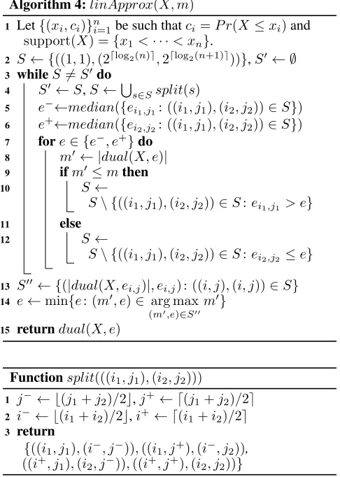
The problem with the saddleback algorithm is that it needs to rundualat every step so it has a quadratic time complex-ity. Since we cannot find the required entry of the matrix in less thannsteps, we can only reduce the complexity by proposing an algorithm that does not executedualin all the steps, only inlog(n)of them. Such an algorithm, based on Section 2.1 of (Fournier and Vigneron 2011), is listed as Algo-rithm 4. The algoAlgo-rithm maintains a setSof sub-matrices of
(ei,j)i=1..2dlog2(n)e,j=1..2dlog2(n+1)e. At each round of its
exe-cution, each sub-matrix is split to four and then about three quarters of the matrix are discarded. At the end, at most four scalar matrices remain containing the index of the entry we seek. Note that this algorithm runs on a matrix that, in the worst case, can be almost four times bigger than the matrix traversed by the saddleback algorithm. This, of course, does not affect the asymptotic complexity, but it may matter when dealing with relatively small random variables.
Theorem 10. linApprox(X, m)∈arg min |X0|≤m
dK(X, X0)
Algorithm 4:linApprox(X, m)
1 Let{(xi, ci)}ni=1be such thatci=P r(X≤xi)and
support(X) ={x1<· · ·< xn}.
2 S← {((1,1),(2dlog2(n)e,2dlog2(n+1)e))},S0← ∅
3 whileS6=S0do
4 S0←S,S←Ss∈Ssplit(s)
5 e−←median({ei1,j1: ((i1, j1),(i2, j2))∈S})
6 e+←median({ei2,j2: ((i1, j1),(i2, j2))∈S})
7 fore∈ {e−, e+}do
8 m0← |dual(X, e)|
9 ifm0≤mthen
10 S←
S\ {((i1, j1),(i2, j2))∈S:ei1,j1 > e}
11 else
12 S←
S\ {((i1, j1),(i2, j2))∈S:ei2,j2 ≤e}
13 S00← {(|dual(X, ei,j)|, ei,j) : ((i, j),(i, j))∈S}
14 e←min{e: (m0, e)∈ arg max (m0,e)∈S00
m0}
15 returndual(X, e)
Functionsplit(((i1, j1),(i2, j2)))
1 j−← b(j1+j2)/2c,j+← d(j
1+j2)/2e 2 i−← b(i1+i2)/2c,i+← d(i1+i2)/2e 3 return
{((i1, j1),(i−, j−)),((i1, j+),(i−, j2)),
((i+, j1),(i2, j−)),((i+, j+),(i2, j2))}
the bottom right) is smaller or equal to an entry that does not meet our condition.
Theorem 11. ThelinApprox(X, m)algorithm runs in time
O(nlog(n)), usingO(1)memory wheren=|X|.
Proof. The dimension of each matrix is halved in each round, thus the loop is executedO(log(n))rounds. Sincedualis called one in each round and a finite number of times at the end, the time complexity isO(nlog(n)).
4
Experimental evaluation
We describe below several experiments that show how
linApproxperforms in practice in different applications and domains. All algorithms were implemented in Python and the experiments were executed on a hardware comprised of an Intel i5-6500 CPU @ 3.20GHz processor and 8GB memory. The algorithms of Cohen et al. were taken “as is” from in the supplementary material to (Cohen, Shimony, and Weiss 2015).
Repetitive support size minimization. One use of sup-port size minimization is when commutations that involve summations of random variables slow due to an exponen-tial growth in the support of convolutions of random vari-ables (Cohen, Shimony, and Weiss 2015). A key action
in coping with this situation is reduction of the support size by replacing the summed random variable by an ap-proximation of it that has a smaller support size. Previ-ous work such as the work of Cohen et al. in (2015; 2018) handle this reduction using weaker or sub-optimal no-tion of approximano-tion than ours.
As we proved above, givenm, a single step oflinApprox
guarantees an optimalm-approximation. However in the set-ting considered here we need to repetitively uselinApprox, thus the optimality of the eventually obtained random vari-able is not guaranteed. In light of this, we tested the ac-curacy of the repetitive-linApproxto see how it performs against the tools of (Cohen, Shimony, and Weiss 2015; Cohen, Grinshpoun, and Weiss 2018) using their benchmarks. These benchmarks are taken from the area of task trees with deadlines, a sub area of the well-established hierarchical planning (Dean, Firby, and Miller 1988; Alford et al. 2016; Xiao et al. 2017).
We estimated the probability for meeting deadlines in plans, as described in Cohen et al. (2015; 2018), and experi-mented with four different methods of approximation. The first two,OptTrim(Cohen, Grinshpoun, and Weiss 2018) and the
Trim(Cohen, Shimony, and Weiss 2015), are taken from the repository provided by the authors and are designed for achiev-ing only a one-sided Kolmogorov approximation - a weaker notion of approximation than the Kolmogorov approximation analyzed in this work. The third method is a simple sampling scheme and the fourth is our Kolmogorov approximation ob-tained by the proposedlinApproxalgorithm. The parameters for the different methods were chosen in a compatible way,
M is the maximal support size,Nis the number of nodes of the plan network andsis the number of samples. We ran also an exact computation as a reference to the approximated one in order to calculate the errors.
Task Tree M linApprox OptTrim Trim Sampling m/N=10 m/N=10 ε·N=0.1 s=104 s=106
Logistics 2 0 0 0.0019 0.007 0.0009
(N= 34) 4 0.0024 0.0046 0.0068 0.0057 0.0005
DRC-Drive 2 0.0014 0.004 0.009 0.0072 0.0009 (N=47) 4 0.001 0.008 0.019 0.0075 0.0011
Sequential 2 0.0093 0.015 0.024 0.0063 0.0008 (N=10) 4 0.008 0.024 0.04 0.008 0.0016
Table 1: Comparison of estimated errors with respect to the reference exact computation on various task trees.
Table 1 shows the results of the experiment. The quality of the solutions obtained with thelinApproxoperator are better than those obtained by theTrimandOptTrimoperators as expected. In some of the task trees, the sampling method produced better results thanlinApprox. Still, thelinApprox
approximation algorithm comes with an inherent advantage of providing exact quality guarantees, as opposed to sampling where the best one can hope for is probabilistic guarantees.
6 10 15 19 10−3
10−2 10−1 100 101 102
Number of variables
Run-time
(seconds)
Exact (no trimming)
OptTrim
n2log(n) binsApprox
nlog(n) linApprox Trim
Figure 1: Run-time of a long computation withlinApprox,
binsApprox,OptTrim,Trim, and without any trimming.
linApprox,binsApprox,OptTrimandTrimas operators. We examined four versions of approximation each of which with different run-time but onlylinApproxandbinsApprox
produce optimal Kolmogorov approximation. The computa-tion is a summacomputa-tion of a sequence of random variables with support size ofm=10, where the numbernof variables varies from 6 to 19. In this experiment, we executed the approxima-tion algorithm withm=10after performing each convolution between two random variables, in order to maintain a sup-port size of 10 in all intermediate computations. Equivalently, we executed the Trimoperator withε = 0.1. The results clearly show the exponential run-time of the exact compu-tation, caused by the convolution between two consecutive random variables. In fact, in the experiment withN=20, the exact computation ran out of memory. These results illumi-nate the advantage of the proposedlinApproxalgorithm that balances between solution quality and run-time performance – while there exist other, faster, methods (e.g.,Trim),linApprox
provides high-quality solutions inO(nlog(n))time, which is especially important when an exact computation is not feasi-ble, due to time or memory. In general, Figure 1 is consistent with the theory and show a good fit to the complexity analysis.
Single step support minimisation. To better understand the quality gaps in practice betweenlinApprox,OptTrim, andTrim, we tested their performance on random variables withn=100, and differentms. Note that the error obtained by linApproxis optimal while the other methods are not optimised for the Kolmogorv distance. In each instance of the experiment, a random variable is randomly generated by choosing the probabilities of each element in the support uniformly and then normalise these probabilities to sum to 1. Figure 2 presents the error produced by the above methods. The depicted results are averages over fifty instances of random variables. The curves in the figure show the average error of
OptTrimandTrimoperators with comparison to the average error of the optimal approximation provided bylinApproxas a function ofm. It is evident from this graphs that increasing
2 4 810 20 50
0 0.2 0.4
Support size,m
Error
,
dK
(
X
,
X
0)
linApprox OptTrim
Trim
Figure 2: Error comparison betweenlinApprox,OptTrim, andTrimon randomly generated variables as function ofm.
the support size of the approximationmreduces the error, as expected, in all three methods. However, the errors produced by thelinApproxare significantly smaller, a half of the error produced byOptTrimandTrim.
Comparison to Linear Programming. We also compared the run-time oflinApproxwith a linear programming (LP) al-gorithm that guarantees optimality, as described and discussed in (Pavlikov and Uryasev 2016). We used the “Minimize” function of Wolfram Mathematica as a state-of-the-art imple-mentation of linear programming, encoding the problem by the LP problemminα∈Rnkx−αk∞subject tokαk0 ≤m
andkαk1=1. The run-time comparison results were clear and
persuasive:linApproxsignificantly outperforms the LP al-gorithm. For a random variable with support sizen=10and
m= 5, the LP algorithm run-time was850seconds, where the linApproxalgorithm run-time was less than a second. Forn=100andm=5, thelinApproxalgorithm run-time was 0.14 seconds and the LP algorithm took more than a day. Since it is not trivial to formally analyze the run-time of the LP al-gorithm, we conclude by the reported experiment that in this case the LP algorithm might not be as efficient aslinApprox.
5
Discussion and future work
We developed an efficient algorithm for computing optimal approximations of random variables where the approximation quality is measured by the Kolmogorov distance. As demon-strated in the experiments, our algorithm improves on the approach of Cohen et al. (2015) and (2018) in that it finds an optimal two sided Kolmogorov approximation, and not just one sided. In addition, the algorithmlinApproxpresented in this paper is very efficient with complexity ofO(nlog(n))as proved in Theorem 11 and showed in Figure 1. Beyond the Kolmogorov measure studied here, we believe that similar ap-proaches may apply also to total variation, to the Wasserstein distance, and to other measures of approximations.
References
Alford, R.; Shivashankar, V.; Roberts, M.; Frank, J.; and Aha, D. W. 2016. Hierarchical planning: Relating task and goal decomposition with task sharing. InIJCAI, 3022–3029. Bolton, C., et al. 2010. Logistic regression and its application in credit scoring. Ph.D. Dissertation, University of Pretoria. Cohen, L.; Grinshpoun, T.; and Weiss, G. 2018. Optimal ap-proximation of random variables for estimating the probability of meeting a plan deadline. InAAAI, 6327–6334.
Cohen, L.; Shimony, S. E.; and Weiss, G. 2015. Estimating the probability of meeting a deadline in hierarchical plans. In
IJCAI, 1551–1557.
Dean, T.; Firby, R. J.; and Miller, D. 1988. Hierarchical planning involving deadlines, travel time, and resources. Com-putational Intelligence4(3):381–398.
D´ıaz-B´anez, J. M., and Mesa, J. A. 2001. Fitting rectilinear polygonal curves to a set of points in the plane. European Journal of Operational Research130(1):214–222.
Fournier, H., and Vigneron, A. 2008. Fitting a step function to a point set. InEuropean Symposium on Algorithms, 442–453. Springer.
Fournier, H., and Vigneron, A. 2011. Fitting a step function to a point set.Algorithmica60(1):95–109.
Gibbons, J. D., and Chakraborti, S. 2011. Nonparametric sta-tistical inference. InInternational encyclopedia of statistical science. Springer. 977–979.
Guha, S., and Shim, K. 2007. A note on linear time algo-rithms for maximum error histograms.IEEE Transactions on Knowledge and Data Engineering19(7):993–997.
Guha, S.; Shim, K.; and Woo, J. 2004. Rehist: Relative error histogram construction algorithms. InVLDB, 300–311. Guha, S. 2008. Posterior simulation in the generalized linear mixed model with semiparametric random effects. J. Comput. Graph. Statist.17(2):410–425.
Jagadish, H. V.; Koudas, N.; Muthukrishnan, S.; Poosala, V.; Sevcik, K. C.; and Suel, T. 1998. Optimal histograms with quality guarantees. InVLDB, volume 98, 24–27.
Karras, P.; Sacharidis, D.; and Mamoulis, N. 2007. Exploiting duality in summarization with deterministic guarantees. In
SIGKDD, 380–389.
Kashef, M., and Moayeri, N. 2018. Random-deadline missing probability analysis for wireless communications in industrial environments. InWFCS, 1–8.
Mays, E. 2001.Handbook of credit scoring. Global Profes-sional Publishi.
Miller, A. C., and Rice, T. R. 1983. Discrete approximations of probability distributions.Management Science29(3):352– 362.
Pavlikov, K., and Uryasev, S. 2016. CVaR distance between univariate probability distributions and approximation prob-lems. Technical Report 2015-6, University of Florida. Pettitt, A. N., and Stephens, M. A. 1977. The kolmogorov-smirnov goodness-of-fit statistic with discrete and grouped data.Technometrics19(2):205–210.
Refaat, M. 2011. Credit Risk Scorecard: Development and Implementation Using SAS. Lulu. com.
Siddiqi, N. 2012. Credit risk scorecards: developing and implementing intelligent credit scoring, volume 3. John Wiley & Sons.
Vidyasagar, M. 2012. A metric between probability distribu-tions on finite sets of different cardinalities and applicadistribu-tions to order reduction. IEEE Transactions on Automatic Control
57(10):2464–2477.
Xiao, Z.; Herzig, A.; Perrussel, L.; Wan, H.; and Su, X. 2017. Hierarchical task network planning with task insertion and state constraints. InIJCAI.