Knowledge Graph Completion via Complex Tensor
Factorization
Th´eo Trouillon [email protected]
Univ. Grenoble Alpes, 700 avenue Centrale, 38401 Saint Martin d’H`eres, France
Christopher R. Dance [email protected]
NAVER LABS Europe, 6 chemin de Maupertuis, 38240 Meylan, France
´
Eric Gaussier [email protected]
Univ. Grenoble Alpes, 700 avenue Centrale, 38401 Saint Martin d’H`eres, France
Johannes Welbl [email protected]
Sebastian Riedel [email protected]
University College London, Gower St, London WC1E 6BT, United Kingdom
Guillaume Bouchard [email protected]
Bloomsbury AI, 115 Hampstead Road, London NW1 3EE, United Kingdom University College London, Gower St, London WC1E 6BT, United Kingdom
Editor:Luc De Raedt
Abstract
In statistical relational learning, knowledge graph completion deals with automati-cally understanding the structure of large knowledge graphs—labeled directed graphs— and predicting missing relationships—labeled edges. State-of-the-art embedding models propose different trade-offs between modeling expressiveness, and time and space complex-ity. We reconcile both expressiveness and complexity through the use of complex-valued embeddings and explore the link between such complex-valued embeddings and unitary diagonalization. We corroborate our approach theoretically and show thatall real square matrices—thus all possible relation/adjacency matrices—are the real part of some unitarily diagonalizable matrix. This results opens the door to a lot of other applications of square matrices factorization. Our approach based on complex embeddings is arguably simple, as it only involves a Hermitian dot product, the complex counterpart of the standard dot product between real vectors, whereas other methods resort to more and more complicated composition functions to increase their expressiveness. The proposed complex embeddings are scalable to large data sets as it remains linear in both space and time, while consistently outperforming alternative approaches on standard link prediction benchmarks.1
Keywords: complex embeddings, tensor factorization, knowledge graph, matrix comple-tion, statistical relational learning
1. Introduction
Web-scale knowledge graph provide a structured representation of world knowledge, with projects such as the Google Knowledge Vault (Dong et al., 2014). They enable a wide range of applications including recommender systems, question answering and automated
1. Code is available at: https://github.com/ttrouill/complex
c
personal agents. The incompleteness of these knowledge graphs—also called knowledge bases—has stimulated research into predicting missing entries, a task known as link pre-diction or knowledge graph completion. The need for high quality predictions required by link prediction applications made it progressively become the main problem in statistical relational learning (Getoor and Taskar, 2007), a research field interested in relational data representation and modeling.
Knowledge graphs were born with the advent of the Semantic Web, pushed by the World Wide Web Consortium (W3C) recommendations. Namely, the Resource Description Frame-work (RDF) standard, that underlies knowledge graphs’ data representation, provides for the first time a common framework across all connected information systems to share their data under the same paradigm. Being more expressive than classical relational databases, all existing relational data can be translated into RDF knowledge graphs (Sahoo et al., 2009).
Knowledge graphs express data as a directed graph with labeled edges (relations) be-tween nodes (entities). Natural redundancies bebe-tween the recorded relations often make it possible to fill in the missing entries of a knowledge graph. As an example, the relation CountryOfBirth could not be recorded for all entities, but it can be inferred if the rela-tion CityOfBirthis known. The goal of link prediction is the automatic discovery of such regularities. However, many relations are non-deterministic: the combination of the two facts IsBornIn(John,Athens) and IsLocatedIn(Athens,Greece) does not always imply the fact HasNationality(John,Greece). Hence, it is natural to handle inference proba-bilistically, and jointly with other facts involving these relations and entities. To this end, an increasingly popular method is to state the knowledge graph completion task as a 3D binary tensor completion problem, where each tensor slice is the adjacency matrix of one relation in the knowledge graph, and compute a decomposition of this partially-observed tensor from which its missing entries can be completed.
Factorization models with low-rank embeddings were popularized by the Netflix chal-lenge (Koren et al., 2009). A partially-observed matrix or tensor is decomposed into a product of embedding matrices with much smaller dimensions, resulting in fixed-dimensional vector representations for each entity and relation in the graph, that allow completion of the missing entries. For a given fact r(s,o) in which the subject entitysis linked to the object entityothrough the relationr, a score for the fact can be recovered as a multilinear product between the embedding vectors of s, r and o, or through more sophisticated composition functions (Nickel et al., 2016a).
and (ir)-reflexivity of relations, and when combined with an appropriate loss function, dot products can even handle transitivity (Bouchard et al., 2015). However, dealing with antisymmetric—and more generally asymmetric—relations has so far almost always implied superlinear time and space complexity (Nickel et al., 2011; Socher et al., 2013) (see Section 2), making models prone to overfitting and not scalable. Finding the best trade-off between expressiveness, generalization and complexity is the keystone of embedding models.
In this work, we argue that the standard dot product between embeddings can be a very effective composition function, provided that one uses the right representation: instead of using embeddings containing real numbers, we discuss and demonstrate the capabilities of complex embeddings. When using complex vectors, that is vectors with entries in C, the
dot product is often called the Hermitian (or sesquilinear) dot product, as it involves the conjugate-transpose of one of the two vectors. As a consequence, the dot product is not symmetric any more, and facts about one relation can receive different scores depending on the ordering of the entities involved in the fact. In summary, complex embeddings naturally represent arbitrary relations while retaining the efficiency of a dot product, that is linearity in both space and time complexity.
This paper extends a previously published article (Trouillon et al., 2016). This extended version adds proofs of existence of the proposed model in both single and multi-relational settings, as well as proofs of the non-uniqueness of the complex embeddings for a given relation. Bounds on the rank of the proposed decomposition are also demonstrated and discussed. The learning algorithm is provided in more details, and more experiments are provided, especially regarding the training time of the models.
The remainder of the paper is organized as follows. We first provide justification and intuition for using complex embeddings in the square matrix case (Section 2), where there is only a single type of relation between entities, and show the existence of the proposed decomposition for all possible relations. The formulation is then extended to a stacked set of square matrices in a third-order tensor to represent multiple relations (Section 3). The stochastic gradient descent algorithm used to learn the model is detailed in Section 4, where we present an equivalent reformulation of the proposed model that involves only real embeddings. This should help practitioners when implementing our method, without requiring the use of complex numbers in their software implementation. We then describe experiments on large-scale public benchmark knowledge graphs in which we empirically show that this representation leads not only to simpler and faster algorithms, but also gives a systematic accuracy improvement over current state-of-the-art alternatives (Section 5). Related work is discussed in Section 6.
2. Relations as the Real Parts of Low-Rank Normal Matrices
We consider in this section a simplified link prediction task with a single relation, and introduce complex embeddings for low-rank matrix factorization.
2.1 Modeling Relations
Let E be a set of entities, with |E| = n. The truth of the single relation holding between two entities is represented by a sign value yso ∈ {−1,1}, where 1 represents true facts and -1 false facts,s∈ E is the subject entity and o∈ E is the object entity. The probability for the relation holding true is given by
P(yso= 1) =σ(xso) (1)
where X ∈ Rn×n is a latent matrix of scores indexed by the subject (rows) and object
entities (columns), Y is a partially-observed sign matrix indexed in identical fashion, and
σ is a suitable sigmoid function. Throughout this paper we used the logistic inverse link functionσ(x) = 1+e1−x.
2.1.1 Handling Both Asymmetry and Unique Entity Embeddings
In this work we pursue three objectives: finding a generic structure for X that leads to (i) a computationally efficient model, (ii) an expressive enough approximation of common relations in real world knowledge graphs, and (iii) good generalization performances in practice. Standard matrix factorization approximatesX by a matrix productU V>, where
U andV are two functionally-independentn×K matrices,K being the rank of the matrix. Within this formulation it is assumed that entities appearing as subjects are different from entities appearing as objects. In the Netflix challenge (Koren et al., 2009) for example, each rowui corresponds to the useriand each columnvj corresponds to the moviej. This
extensively studied type of model is closely related to the singular value decomposition (SVD) and fits well with the case where the matrixX is rectangular.
However, in many knowledge graph completion problems, the same entity i can ap-pear as both subject or object and will have two different embedding vectors, ui and vi, depending on whether it appears as subject or object of a relation. It seems natural to learn unique embeddings of entities, as initially proposed by Nickel et al. (2011) and Bordes et al. (2011) and since then used systematically in other prominent approaches (Bordes et al., 2013b; Yang et al., 2015; Socher et al., 2013). In the factorization setting, using the same embeddings for left- and right-side factors boils down to a specific case of eigenvalue decomposition: orthogonal diagonalization.
Definition 1 A real square matrix X ∈ Rn×n is orthogonally diagonalizable if it can be
written as X = EW E>, where E, W ∈ Rn×n, W is diagonal, and E orthogonal so that EE>=E>E =I where I is the identity matrix.
The spectral theorem for symmetric matrices tells us that a matrix is orthogonally diagonalizable if and only if it is symmetric (Cauchy, 1829). It is therefore often used to approximate covariance matrices, kernel functions and distance or similarity matrices.
Model Scoring Functionφ Relation Parameters Otime Ospace
CP (Hitchcock, 1927) hwr, us, voi wr∈RK O(K) O(K)
RESCAL (Nickel et al., 2011) eT
sWreo Wr∈RK
2
O(K2) O(K2)
TransE (Bordes et al.,
2013b) −||(es+wr)−eo||p wr∈R
K O(K) O(K)
NTN (Socher et al., 2013) u>rf(esW
[1..D]
r eo+Vr
es eo
+br) Wr∈R K2D
, br∈RK
Vr∈R2KD, ur∈RK
O(K2D) O(K2D)
DistMult(Yang et al., 2015) hwr, es, eoi wr∈RK O(K) O(K)
HolE(Nickel et al., 2016b) wT
r(F−1[F[es] F[eo]])) wr∈RK O(KlogK) O(K)
ComplEx(this paper) Re(hwr, es,¯eoi) wr∈CK O(K) O(K)
Table 1: Scoring functions of state-of-the-art latent factor models for a given fact r(s, o), along with the representation of their relation parameters, and time and space (memory) complexity. K is the dimensionality of the embeddings. The entity embeddingses and eo of subject sand objecto are inRK for each model, except
for ComplEx, where es, eo ∈ CK. x¯ is the complex conjugate, and D is an
additional latent dimension of the NTN model. F and F−1 denote respectively the Fourier transform and its inverse,is the element-wise product between two vectors, Re(.) denotes the real part of a complex vector, and h·,·,·i denotes the trilinear product.
composition functions, that allow more general combinations of embeddings. We briefly recall several examples of scoring functions in Table 1, as well as the extension proposed in this paper.
These models propose different trade-offs between the three essential points:
• Expressiveness, which is the ability to represent symmetric, antisymmetric and more generally asymmetric relations.
• Scalability, which means keeping linear time and space complexity scoring function.
• Generalization, for which having unique entity embeddings is critical.
RESCAL (Nickel et al., 2011) and NTN (Socher et al., 2013) are very expressive, but their scoring functions have quadratic complexity in the rank of the factorization. More recently the HolE model (Nickel et al., 2016b) proposes a solution that has quasi-linear
complexity in time and linear space complexity. DistMult(Yang et al., 2015) can be seen
as a joint orthogonal diagonalization with real embeddings, hence handling only symmetric relations. Conversely, TransE (Bordes et al., 2013b) handles symmetric relations to the
price of strong constraints on its embeddings. The canonical-polyadic decomposition (CP) (Hitchcock, 1927) generalizes poorly with its different embeddings for entities as subject and as object.
2.1.2 Decomposition in the Complex Domain
We introduce a new decomposition of real square matrices using unitary diagonalization, the generalization of orthogonal diagonalization to complex matrices. This allows decom-position ofarbitrary real square matrices with unique representations of rows and columns. Let us first recall some notions of complex linear algebra as well as specific cases of diagonalization of real square matrices, before building our proposition upon these results. A complex-valued vector x ∈CK, with x = Re(x) +iIm(x) is composed of a real part
Re(x)∈RK and an imaginary part Im(x)∈
RK, whereidenotes the square root of−1. The
conjugatexof a complex vector inverts the sign of its imaginary part: x= Re(x)−iIm(x). Conjugation appears in the usual dot product for complex numbers, called theHermitian product, orsesquilinear form, which is defined as:
hu, vi := u¯>v
= Re(u)>Re(v) + Im(u)>Im(v) +i(Re(u)>Im(v)−Im(u)>Re(v)).
A simple way to justify the Hermitian product for composing complex vectors is that it provides a valid topological norm in the induced vector space. For example, ¯x>x = 0 impliesx= 0 while this is not the case for the bilinear formx>xas there are many complex vectors xfor which x>x= 0.
This yields an interesting property of the Hermitian product concerning the order of the involved vectors: hu, vi =hv, ui, meaning that the real part of the product is symmetric, while the imaginary part is antisymmetric.
For matrices, we shall write X∗∈Cn×m for the conjugate-transposeX∗ = (X)>=X>.
The conjugate transpose is also often writtenX† orXH.
Definition 2 A complex square matrix X ∈ Cn×n is unitarily diagonalizable if it can be
written as X = EW E∗, where E, W ∈ Cn×n, W is diagonal, and E is unitary such that EE∗ =E∗E =I.
Definition 3 A complex square matrix X is normal if it commutes with its conjugate-transpose so that XX∗=X∗X.
We can now state the spectral theorem for normal matrices.
Theorem 1 (Spectral theorem for normal matrices, von Neumann (1929)) LetX
be a complex square matrix. Then X is unitarily diagonalizable if and only if X is normal.
As we only focus on real square matrices in this work, let us summarize all the cases whereXis real square andX =EW E∗ifXis unitarily diagonalizable, whereE, W ∈Cn×n, W is diagonal and E is unitary:
• X is symmetric if and only if X is orthogonally diagonalizable and E and W are purely real.
• Xis normal and non-symmetric if and only ifX is unitarily diagonalizable andE and
W arenot both purely real.
• X is not normal if and only if X is not unitarily diagonalizable.
We generalize all three cases by showing that, for anyX ∈Rn×n, there exists a unitary
diagonalization in the complex domain, of which the real part equalsX:
X= Re(EW E∗). (2)
In other words, the unitary diagonalization is projected onto the real subspace.
Theorem 2 Suppose X∈Rn×n is a real square matrix. Then there exists a normal matrix Z ∈Cn×n such that Re(Z) =X.
Proof Let Z :=X+iX>. Then
Z∗ =X>−iX =−i(iX>+X) =−iZ ,
so that
ZZ∗=Z(−iZ) = (−iZ)Z =Z∗Z .
ThereforeZ is normal.
Note that there also exists a normal matrixZ =X>+iX such that Im(Z) =X.
Following Theorem 1 and Theorem 2, any real square matrix can be written as the real part of a complex diagonal matrix through a unitary change of basis.
Corollary 1 Suppose X ∈Rn×n is a real square matrix. Then there exist E, W ∈ Cn×n,
where E is unitary, and W is diagonal, such thatX= Re(EW E∗).
Proof From Theorem 2, we can write X= Re(Z), where Z is a normal matrix, and from Theorem 1,Z is unitarily diagonalizable.
Applied to the knowledge graph completion setting, the rows of E here are vectorial representations of the entities corresponding to rows and columns of the relation score matrixX. The score for the relation holding true between entities sand ois hence
xso= Re(e>sWe¯o) (3)
where es, eo ∈ Cn and W ∈ Cn×n is diagonal. For a given entity, its subject embedding
To illustrate this difference of expressiveness with respect to real-valued embeddings, let us consider two complex embeddings es, eo ∈C of dimension 1, with arbitrary values: es = 1−2i, and eo = −3 + i; as well as their real-valued, twice-bigger counterparts: e0s = 1
−2
∈ R2 and e0
o = −13
∈ R2. In the real-valued case, that corresponds to the
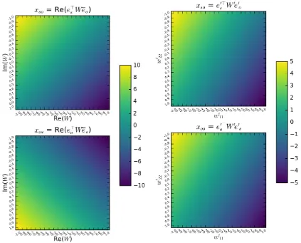
DistMult model (Yang et al., 2015), the score is xso =e0>s W0e0o. Figure 1 represents the
heatmaps of the scoresxsoandxos, as a function ofW ∈Cin the complex-valued case, and
as a function of W0 ∈R2 diagonal in the real-valued case. In the real-valued case, that is symmetric in the subject and object entities, the scoresxso and xos are equal for any value of W0 ∈R2 diagonal. Whereas in the complex-valued case, the variation of W ∈
C allows
to scorexso andxos with any desired pair of values.
This decomposition however is non-unique, a simple example of this non-uniqueness is obtained by adding a purely imaginary constant to the eigenvalues. Let X ∈ Rn×n, and X = Re(EW E∗) where E is unitary, W is diagonal. Then for any real constant c ∈Rwe have:
X = Re(E(W +icI)E∗) = Re(EW E∗+icEIE∗) = Re(EW E∗+icI) = Re(EW E∗).
In general, there are many other possible couples of matricesE andW that preserve the real part of the decomposition. In practice however this is no synonym of low generaliza-tion abilities, as many effective matrix and tensor decomposigeneraliza-tion methods used in machine learning lead to non-unique solutions (Paatero and Tapper, 1994; Nickel et al., 2011). In this case also, the learned representations prove useful as shown in the experimental section.
2.2 Low-Rank Decomposition
Addressing knowledge graph completion with data-driven approaches assumes that there is a sufficient regularity in the observed data to generalize to unobserved facts. When formulated as a matrix completion problem, as it is the case in this section, one way of implementing this hypothesis is to make the assumption that the matrix has a low rank or approximately low rank. We first discuss the rank of the proposed decomposition, and then introduce the sign-rank and extend the bound developed on the rank to the sign-rank.
2.2.1 Rank Upper Bound
First, we recall one definition of the rank of a matrix (Horn and Johnson, 2012).
Definition 4 The rank of an m-by-n complex matrix rank(X) = rank(X>) =k, if X has exactlyk linearly independent columns.
Also note that if X is diagonalizable so thatX=EW E−1 with rank(X) =k, thenW
hask non-zero diagonal entries for some diagonal W and some invertible matrix E. From this it is easy to derive a known additive property of the rank:
Figure 1: Left: Scores xso = Re(e>sW¯eo) (top) and xos = Re(e>oW es) (bottom) for the
proposed complex-valued decomposition, plotted as a function ofW ∈C, for fixed entity embeddingses = 1−2i, andeo=−3+i. Right: Scoresxso=e0>s W0e0o(top)
and xos = e0>o W0e0s (bottom) for the corresponding real-valued decomposition
with the same number of free real-valued parameters (i.e. in twice the dimension), plotted as a function ofW0 ∈R2 diagonal, for fixed entity embeddingse0
s= −12
ande0o= −3 1
. By varying W ∈C, the proposed complex-valued decomposition
can attribute any pair of scores toxsoand xos, whereasxso=xos for allW0 ∈R2 with the real-valued decomposition.
whereB, C ∈Cm×n.
We now show that any rank k real square matrix can be reconstructed from a 2k -dimensional unitary diagonalization.
Corollary 2 Suppose X ∈ Rn×n and rank(X) = k. Then there exist E ∈
Cn×2k such
Proof Consider the complex square matrix Z := X +iX>. We have rank(iX>) = rank(X>) = rank(X) =k.
From Equation (4), rank(Z)≤rank(X) + rank(iX>) = 2k.
The proof of Theorem 2 shows that Z is normal. Thus Z =EW E∗ with E ∈ Cn×2k, W ∈C2k×2kwhere the columns ofEform an orthonormal basis ofC2k, andW is diagonal.
Since E is not necessarily square, we replace the unitary requirement of Corollary 1 by the requirement that its columns form an orthonormal basis of its smallest dimension, 2k.
Also, given that such decomposition always exists in dimension n (Theorem 2), this upper bound is not relevant when rank(X)≥ n2.
2.2.2 Sign-Rank Upper Bound
Since we encode the truth values of each fact with ±1, we deal with square sign matrices:
Y ∈ {−1,1}n×n. Sign matrices have an alternative rank definition, thesign-rank.
Definition 5 The sign-rank rank±(Y) of an m-by-n sign matrix Y, is the rank of the m
-by-n real matrix of least rank that has the same sign-pattern as Y, so that
rank±(Y) := min X∈Rm×n
{rank(X)|sign(X) =Y},
where sign(X)ij = sign(xij).
We define the sign function ofc∈R as
sign(c) =
1 ifc≥0 −1 otherwise
where the valuec= 0 is here arbitrarily assigned to 1 to allow zero entries inX, conversely to the stricter usual definition of the sign-rank.
To make generalization possible, we hypothesize that the true matrixY has a low sign-rank, and thus can be reconstructed by the sign of a low-rank score matrix X. The low sign-rank assumption is theoretically justified by the fact that the sign-rank is a natural complexity measure of sign matrices (Linial et al., 2007) and is linked to learnability (Alon et al., 2016) and empirically confirmed by the wide success of factorization models (Nickel et al., 2016a).
Using Corollary 2, we can now show that any square sign matrix of sign-rank kcan be reconstructed from a rank 2k unitary diagonalization.
Corollary 3 Suppose Y ∈ {−1,1}n×n, rank
±(Y) = k. Then there exists E ∈ Cn×2k, W ∈C2k×2k where the columns of E form an orthonormal basis of
C2k, and W is diagonal,
such that Y = sign(Re(EW E∗)).
Proof By definition, if rank±(Y) = k, there exists a real square matrix X such that
rank(X) = k and sign(X) = Y. From Corollary 2, X = Re(EW E∗) where E ∈ Cn×2k, W ∈C2k×2kwhere the columns ofEform an orthonormal basis of
Previous attempts to approximate the sign-rank in relational learning did not use com-plex numbers. They showed the existence of compact factorizations under conditions on the sign matrix (Nickel et al., 2014), or only in specific cases (Bouchard et al., 2015). In contrast, our results show that if a square sign matrix has sign-rankk, then it can be exactly decomposed through a 2k-dimensional unitary diagonalization.
Although we can only show the existence of a complex decomposition of rank 2kfor a matrix with sign-rankk, the sign rank ofY is often much lower than the rank ofY, as we do not know any matrixY ∈ {−1,1}n×n for which rank
±(Y)>
√
n(Alon et al., 2016). For example, the n×n identity matrix has rank n, but its sign-rank is only 3! By swapping the columns 2j and 2j−1 forj in 1, . . . ,n2, the identity matrix corresponds to the relation marriedTo, a relation known to be hard to factorize over the reals (Nickel et al., 2014), since the rank is invariant by row/column permutations. Yet our model can express it at most in rank 6, for anyn.
Hence, by enforcing a low-rank K n on EW E∗, individual relation scores xso = Re(e>sW¯eo) between entities s and o can be efficiently predicted, as es, eo ∈ CK and W ∈ CK×K is diagonal.
Finding the K that matches the sign-rank of Y corresponds to finding the smallest K
that brings the 0–1 loss on X to 0, as link prediction can be seen as binary classification of the facts. In practice, and as classically done in machine learning to avoid this NP-hard problem, we use a continuous surrogate of the 0–1 loss, in this case the logistic loss as described in Section 4, and validate models on different values ofK, as described in Section 5.
2.2.3 Rank Bound Discussion
Corollaries 2 and 3 use the aforementioned subadditive property of the rank to derive the 2k upper bound. Let us give an example for which this bound is strictly greater than k.
Consider the following 2-by-2 sign matrix:
Y =
−1 −1 1 1
.
Not only is this matrix not normal, but one can also easily check that there is no real normal 2-by-2 matrix that has the same sign-pattern as Y. Clearly, Y is a rank 1 matrix since its columns are linearly dependent, hence its sign-rank is also 1. From Corollary 3, we know that there is a normal matrix whose real part has the same sign-pattern asY, and whose rank is at most 2.
However, there is no rank 1 unitary diagonalization of which the real part equals Y. Otherwise we could find a 2-by-2 complex matrixZ such that Re(z11)<0 and Re(z22)>0, where z11 = e1we¯1 = w|e1|2, z22 = e2w¯e2 = w|e2|2, e ∈ C2, w ∈ C. This is obviously
unsatisfiable. This example generalizes to any n-by-nsquare sign matrix that only has−1 on its first row and is hence rank 1, the same argument holds considering Re(z11)<0 and Re(znn)>0.
an imaginary part could—additionally to making the matrix normal—create some linear dependence between the rows/columns and thus decrease the rank of the matrix, up to a factor of 2.
We summarize this section in three points:
1. The proposed factorization encompasses all possible score matrices X for a single binary relation.
2. By construction, the factorization is well suited to represent both symmetric and antisymmetric relations.
3. Relation patterns can be efficiently approximated with a low-rank factorization using complex-valued embeddings.
3. Extension to Multi-Relational Data
Let us now extend the previous discussion to models with multiple relations. Let R be the set of relations, with |R|=m. We shall now write X∈ Rm×n×n for the score tensor, Xr ∈ Rn×n for the score matrix of the relation r ∈ R, and Y ∈ {−1,1}m×n×n for the
partially-observed sign tensor.
Given one relation r ∈ Rand two entities s, o ∈ E, the probability that the fact r(s,o) is true given by:
P(yrso= 1) =σ(xrso) =σ(φ(r, s, o; Θ)) (5)
whereφis the scoring function of the model considered and Θ denotes the model parameters. We denote the set of all possible facts (or triples) for a knowledge graph byT =R × E × E. While the tensor X as a whole is unknown, we assume that we observe a set of true and false triples Ω ={((r, s, o), yrso)|(r, s, o) ∈ TΩ} whereyrso ∈ {−1,1} andTΩ ⊆ T is the set of observed triples. The goal is to find the probabilities of entriesyr0s0o0 for a set of targeted
unobserved triples {(r0, s0, o0)∈ T \ TΩ}.
Depending on the scoring function φ(r, s, o; Θ) used to model the score tensor X, we obtain different models. Examples of scoring functions are given in Table 1.
3.1 Complex Factorization Extension to Tensors
The single-relation model is extended by jointly factorizing all the square matrices of scores into a 3rd-order tensorX∈Rm×n×n, with a different diagonal matrixWr ∈CK×K for each
relationr, and by sharing the entity embeddingsE ∈Cn×K across all relations:
φ(r, s, o; Θ) = Re(e>sWreo¯ )
= Re(
K X
k=1
wrkesk¯eok)
= Re(hwr, es,eo¯ i) (6)
where K is the rank hyperparameter, es, eo ∈CK are the rows in E corresponding to the
entities sand o,wr = diag(Wr)∈CK is a complex vector, and ha, b, ci:=P
component-wise multilinear dot product2. For this scoring function, the set of parameters Θ is {ei, wr ∈ CK, i ∈ E, r ∈ R}. This resembles the real part of a complex matrix
decomposition as in the single-relation case discussed above. However, we now have a different vector of eigenvalues for every relation. Expanding the real part of this product gives:
Re(hwr, es,e¯oi) = hRe(wr),Re(es),Re(eo)i
+hRe(wr),Im(es),Im(eo)i
+hIm(wr),Re(es),Im(eo)i
− hIm(wr),Im(es),Re(eo)i. (7)
These equations provide two interesting views of the model:
• Changing the representation: Equation (6) would correspond to DistMultwith real
embeddings (see Table 1), but handles asymmetry thanks to the complex conjugate of the object-entity embedding.
• Changing the scoring function: Equation (7) only involves real vectors corresponding to the real and imaginary parts of the embeddings and relations.
By separating the real and imaginary parts of the relation embedding wr as shown
in Equation (7), it is apparent that these parts naturally act as weights on each latent dimension: Re(wr) over the real part of heo, esi which is symmetric, and Im(w) over the imaginary part ofheo, esi which is antisymmetric.
Indeed, the decomposition of each score matrix Xr for each r ∈ R can be written as the sum of a symmetric matrix and an antisymmetric matrix. To see this, let us rewrite the decomposition of each score matrix Xr in matrix notation. We write the real part of
matrices with primes E0= Re(E) and imaginary parts with double primes E00= Im(E):
Xr = Re(EWrE∗)
= Re((E0+iE00)(Wr0+iWr00)(E0−iE00)>)
= (E0Wr0E0>+E00Wr0E00>) + (E0Wr00E00>−E00Wr00E0>). (8)
It is trivial to check that the matrix E0Wr0E0> +E00Wr0E00> is symmetric and that the matrixE0Wr00E00>−E00Wr00E0> is antisymmetric. Hence this model is well suited to model jointly symmetric and antisymmetric relations between pairs of entities, while still using the same entity representations for subjects and objects. When learning, it simply needs to collapse Wr00= Im(Wr) to zero for symmetric relationsr ∈ R, andWr0 = Re(Wr) to zero for antisymmetric relations r∈ R, asXr is indeed symmetric when Wr is purely real, and antisymmetric whenWr is purely imaginary.
From a geometrical point of view, each relation embedding wr is an anisotropic scaling of the basis defined by the entity embeddings E, followed by a projection onto the real subspace.
3.2 Existence of the Tensor Factorization
Let us first discuss the existence of the multi-relational model where the rank of the decom-positionK ≤n, which relates to simultaneous unitary decomposition.
Definition 6 A family of matrices X1, . . . , Xm ∈ Cn×n is simultaneously unitarily
diago-nalizable, if there is a single unitary matrix E ∈Cn×n, such that Xi =EWiE∗ for all i in
1, . . . , m, where Wi ∈Cn×n are diagonal.
Definition 7 A family of normal matrices X1, . . . , Xm ∈ Cn×n is a commuting family of
normal matrices, if XiXj∗ =Xi∗Xj, for all i, j in 1, . . . , m.
Theorem 3 (see Horn and Johnson (2012)) Suppose F is the family of matrices X1,
. . . , Xm ∈ Cn×n. Then F is a commuting family of normal matrices if and only if F is
simultaneously unitarily diagonalizable.
To apply Theorem 3 to the proposed factorization, we would have to make the hypothesis that the relation score matricesXrare a commuting family, which is too strong a hypothesis.
Actually, the model is slightly different since we take only the real part of the tensor factorization. In the single-relation case, taking only the real part of the decomposition rids us of the normality requirement of Theorem 1 for the decomposition to exist, as shown in Theorem 2.
In the multiple-relation case, it is an open question whether taking the real part of the simultaneous unitary diagonalization will enable us to decompose families of arbitrary real square matrices—that is with a single unitary matrixE that has at most n columns. Though it seems unlikely, we could not find a counter-example yet.
However, by letting the rank of the tensor factorization K to be greater than n, we can show that the proposed tensor decomposition exists for families of arbitrary real square matrices, by simply concatenating the decomposition of Theorem 2 of each real square matrixXi.
Theorem 4 Suppose X1, . . . , Xm ∈ Rn×n. Then there exists E ∈ Cn×nm and Wi ∈ Cnm×nm are diagonal, such that Xi = Re(EWiE∗) for alli in 1, . . . , m.
Proof From Theorem 2 we have Xi = Re(EiWiEi∗), where Wi ∈ Cn×n is diagonal, and
each Ei ∈Cn×n is unitary for alliin 1, . . . , m.
Let E= [E1. . . Em], and
Λi=
0((i−1)n)×((i−1)n) Wi
0((m−i)n)×((m−i)n)
where0l×l the zerol×lmatrix. Therefore Xi= Re(EΛiE∗) for alliin 1, . . . , m.
of relations and n to the number of entities, m is always smaller than n in real world knowledge graphs, hence the bound holds in practice.
Though when it comes to relational learning, we might expect the actual rank to be much lower than nm for two reasons. The first one, as discussed above, is that we are dealing with sign tensors, hence the rank of the matricesXr need only match the sign-rank
of the partially-observed matrices Yr. The second one is that the matrices are related to each other, as they all represent the same entities in different relations, and thus benefit from sharing latent dimensions. As opposed to the construction exposed in the proof of Theorem 4, where other relations dimensions are canceled out. In practice, the rank needed to generalize well is indeed much lower than nmas we show experimentally in Figure 5.
Also, note that with the construction of the proof of Theorem 4, the matrix E = [E1. . . Em] is not unitary any more. However the unitary constraints in the matrix case
serve only the proof of existence, which is just one solution among the infinite ones of same rank. In practice, imposing orthonormality is essentially a numerical commodity for the decomposition of dense matrices, through iterative methods for example (Saad, 1992). When it comes to matrix and tensor completion, and thus generalisation, imposing such constraints is more of a numerical hassle than anything else, especially for gradient methods. As there is no apparent link between orthonormality and generalisation properties, we did not impose these constraints when learning this model in the following experiments.
4. Algorithm
Algorithm 1 describes stochastic gradient descent (SGD) to learn the proposed multi-relational model with the AdaGrad learning-rate updates (Duchi et al., 2011). We refer to the proposed model asComplEx, for Complex Embeddings. We expose a version of the
algorithm that uses only real-valued vectors, in order to facilitate its implementation. To do so, we use separate real-valued representations of the real and imaginary parts of the embeddings.
These real and imaginary part vectors are initialized with vectors having a zero-mean normal distribution with unit variance. If the training set Ω contains only positive triples, negatives are generated for each batch using thelocal closed-world assumption as in Bordes et al. (2013b). That is, for each triple, we randomly change either the subject or the object, to form a negative example. In this case the parameter η >0 sets the number of negative triples to generate for each positive triple. Collision with positive triples in Ω is not checked, as it occurs rarely in real world knowledge graphs as they are largely sparse, and may also be computationally expensive.
Squared gradients are accumulated to compute AdaGrad learning rates, then gradients are updated. Every s iterations, the parameters Θ are evaluated over the evaluation set Ωv (evaluate AP or MRR(Ωv; Θ) function in Algorithm 1). If the data set contains both
Bern(p) is the Bernoulli distribution, the one random sample(E) function sample uni-formly one entity in the set of all entities E, and the sample batch of size b(Ω, b) function sample btrue and false triples uniformly at random from the training set Ω.
For a given embedding size K, let us rewrite Equation (7), by denoting the real part of embeddings with primes and the imaginary part with double primes: e0i = Re(ei), e00i =
Im(ei),w0r = Re(wr),w00r = Im(wr). The set of parameters is Θ ={e0i, e00i, w0r, wr00∈RK, i∈
E, r∈ R}, and the scoring function involves only real vectors:
φ(r, s, o; Θ) = w0r, e0s, eo0+wr0, e00s, e00o
+
w00r, e0s, e00o
−
wr00, e00s, e0o
(9)
where each entity and each relation has two real embeddings. Gradients are now easy to write:
∇e0
sφ(r, s, o; Θ) = (w
0 re
0 o) + (w
00 r e
00 o),
∇e00
sφ(r, s, o; Θ) = (w
0
re00o)−(wr00e0o),
∇e0
oφ(r, s, o; Θ) = (w
0
re0s)−(wr00e00s),
∇e00
oφ(r, s, o; Θ) = (w
0
re00s) + (wr00e0s),
∇w0
rφ(r, s, o; Θ) = (e
0 s e
0 o) + (e
00 s e
00 o),
∇w00
rφ(r, s, o; Θ) = (e
0 s e
00 o)−(e
00 s e
0 o),
where is the element-wise (Hadamard) product.
We optimized the negative log-likelihood of the logistic model described in Equation (5) withL2 regularization on the parameters Θ:
γ(Ω; Θ) = X ((r,s,o),y)∈Ω
log(1 + exp(−yφ(r, s, o; Θ))) +λ||Θ||22 (10)
whereλ∈R+ is the regularization parameter.
To handle regularization, note that using separate representations for the real and imagi-nary parts does not change anything as the squaredL2-norm of a complex vectorv=v0+iv00
is the sum of the squared modulus of each entry:
||v||22 = X
j q
v0j2+v00j2
2
= X
j
vj02+X
j v00j2
= ||v0||22+||v00||22,
which is actually the sum of theL2-norms of the vectors of the real and imaginary parts. We can finally write the gradient of γ with respect to areal embeddingv for one triple (r, s, o) and its truth value y:
Algorithm 1 Stochastic gradient descent with AdaGrad for theComplEx model
Input Training set Ω, validation set Ωv, learning rate α ∈ R++, rank K ∈ Z++, L2
regularization factor λ ∈ R+, negative ratio η ∈ Z++, batch size b ∈ Z++, maximum iteration m∈Z++, validate everys∈Z++ iterations, AdaGrad regularizer= 10−8. Output Embeddingse0, e00, w0, w00.
e0i ∼ N(0k, Ik×k) , e00i ∼ N(0k, Ik×k) for each i∈ E
wi0 ∼ N(0k, Ik×k),w00i ∼ N(0k, Ik×k) for each i∈ R
ge0
i ←0
k ,g e00
i ←0
k for each i∈ E
gw0
i ←0
k ,g
w00i ←0k for each i∈ R previous score←0
for i= 1, . . . , m do forj= 1, . . . ,|Ω|/b do
Ωb ←sample batch of size b(Ω, b)
// Negative sampling: Ωn← {∅}
for((r, s, o), y) in Ωb do for l= 1, . . . , η do
e← one random sample(E) if Bern(0.5)>0.5then
Ωn←Ωn∪ {((r, e, o),−1)} else
Ωn←Ωn∪ {((r, s, e),−1)} end if
end for end for Ωb ←Ωb∪Ωn
for((r, s, o), y) in Ωb do for v in Θdo
// AdaGrad updates:
gv ←gv+ (∇vγ({((r, s, o), y)}; Θ))2 // Gradient updates:
v←v−gα
v+∇vγ({((r, s, o), y)}; Θ)
end for end for end for
// Early stopping if i mod s= 0then
current score← evaluate AP or MRR(Ωv; Θ) if current score≤previous scorethen
break end if
previous score←current score end if
5. Experiments
We evaluated the method proposed in this paper on both synthetic and real data sets. The synthetic data set contains both symmetric and antisymmetric relations, whereas the real data sets are standard link prediction benchmarks based on real knowledge graphs.
We compared ComplEx to state-of-the-art models, namely TransE (Bordes et al.,
2013b), DistMult (Yang et al., 2015), RESCAL (Nickel et al., 2011) and also to the
canonical polyadic decomposition (CP) (Hitchcock, 1927), to emphasize empirically the im-portance of learning unique embeddings for entities. For experimental fairness, we reimple-mented these models within the same framework as theComplExmodel, using a
Theano-based SGD implementation3 (Bergstra et al., 2010).
For the TransE model, results were obtained with its original max-margin loss, as it
turned out to yield better results for this model only. To use this max-margin loss on data sets with observed negatives (Sections 5.1 and 5.2), positive triples were replicated when necessary to match the number of negative triples, as described in Garcia-Duran et al. (2016). All other models are trained with the negative log-likelihood of the logistic model (Equation (10)). In all the following experiments we used a maximum number of iterations
m = 1000, a batch sizeb = 100|Ω|, and validated the models for early stopping every s= 50 iterations.
5.1 Synthetic Task
To assess our claim that ComplEx can accurately model jointly symmetry and
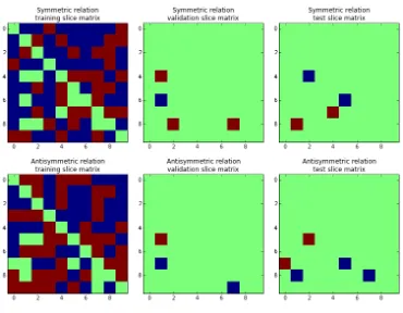
antisym-metry, we randomly generated a knowledge graph of two relations and 30 entities. One relation is entirely symmetric, while the other is completely antisymmetric. This data set corresponds to a 2×30×30 tensor. Figure 2 shows a part of this randomly generated tensor, with a symmetric slice and an antisymmetric slice, decomposed into training, val-idation and test sets. To ensure that all test values are predictable, the upper triangular parts of the matrices are always kept in the training set, and the diagonals are unobserved. We conducted a 5-fold cross-validation on the lower-triangular matrices, using the upper-triangular parts plus 3 folds for training, one fold for validation and one fold for testing. Each training set contains 1392 observed triples, whereas validation and test sets contain 174 triples each.
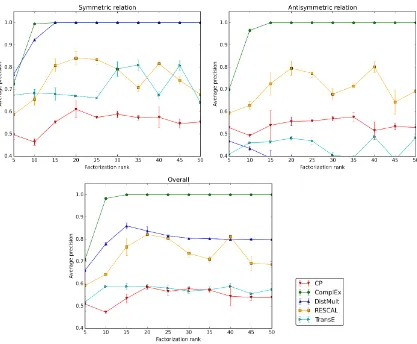
Figure 3 shows the best cross-validated average precision (area under the precision-recall curve) for different factorization models of ranks ranging up to 50. The regularization parameter λ is validated in {0.1, 0.03, 0.01, 0.003,0.001, 0.0003, 0.00001, 0.0} and the learning rateα was initialized to 0.5.
As expected, DistMult (Yang et al., 2015) is not able to model antisymmetry and
only predicts the symmetric relations correctly. Although TransE (Bordes et al., 2013b)
is not a symmetric model, it performs poorly in practice, particularly on the antisymmetric relation. RESCAL (Nickel et al., 2011), with its large number of parameters, quickly overfits as the rank grows. Canonical Polyadic (CP) decomposition (Hitchcock, 1927) fails on both relations as it has to push symmetric and antisymmetric patterns through the entity embeddings. Surprisingly, onlyComplEx succeeds even on such simple data.
Figure 2: Parts of the training, validation and test sets of the generated experiment with one symmetric and one antisymmetric relation. Red pixels are positive triples, blue are negatives, and green missing ones. Top: Plots of the symmetric slice (relation) for the 10 first entities. Bottom: Plots of the antisymmetric slice for the 10 first entities.
5.2 Real Fully-Observed Data Sets: Kinships and UMLS
We then compare all models on two fully observed data sets, that contain both positive and negative triples, also called the closed-world assumption. The Kinships data set (Den-ham, 1973) describes the 26 different kinship relations of the Alyawarra tribe in Australia, among 104 individuals. The unified medical language system (UMLS) data set (McCray, 2003) represents 135 medical concepts and diseases, linked by 49 relations describing their interactions. Metadata for the two data sets is summarized in Table 2.
Data set |E| |R| Total number of triples Kinships 104 26 281,216
UMLS 135 49 893,025
Figure 3: Average precision (AP) for each factorization rank ranging from 5 to 50 for differ-ent state-of-the-art models on the synthetic task. Learning is performed jointly on the symmetric relation and on the antisymmetric relation. Top-left: AP over the symmetric relation only. Top-right: AP over the antisymmetric relation only. Bottom: Overall AP.
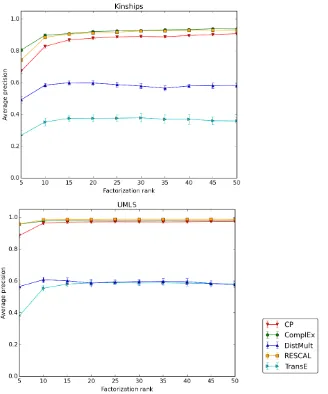
We performed a 10-fold cross-validation, keeping 8 for training, one for validation and one for testing. Figure 4 shows the best cross-validated average precision for ranks ranging up to 50, and error bars show the standard deviation over the 10 runs. The regularization parameter λ is validated in {0.1, 0.03, 0.01, 0.003, 0.001, 0.0003, 0.00001, 0.0} and the learning rateα was initialized to 0.5.
On both data setsComplEx, RESCAL and CP are very close, with a slight advantage
forComplEx on Kinships, and for RESCAL on UMLS. DistMultperforms poorly here
as many relations are antisymmetric both in UMLS (causal links, anatomical hierarchies) and Kinships (being father, uncle or grand-father).
The fact that CP, RESCAL and ComplEx work so well on these data sets
Figure 4: Average precision (AP) for each factorization rank ranging from 5 to 50 for dif-ferent state-of-the-art models on the Kinships data set (top) and on the UMLS data set (bottom).
of antisymmetry; the power of the multilinear product—that is the tensor factorization approach—as TransE can be seen as a sum of bilinear products (Garcia-Duran et al.,
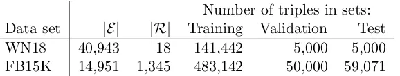
Number of triples in sets: Data set |E| |R| Training Validation Test WN18 40,943 18 141,442 5,000 5,000 FB15K 14,951 1,345 483,142 50,000 59,071
Table 3: Number of entities |E|, relations |R|, and observed triples in each split for the FB15K and WN18 data sets.
5.3 Real Sparse Data Sets: FB15K and WN18
Finally, we evaluated ComplEx on the FB15K and WN18 data sets, as they are well
es-tablished benchmarks for the link prediction task. FB15K is a subset of Freebase (Bollacker et al., 2008), a curated knowledge graph of general facts, whereas WN18 is a subset of Word-Net (Fellbaum, 1998), a database featuring lexical relations between words. We used the same training, validation and test set splits as in Bordes et al. (2013b). Table 3 summarizes the metadata of the two data sets.
5.3.1 Experimental Setup
As both data sets contain only positive triples, we generated negative samples using the local closed-world assumption, as described in Section 4. For evaluation, we measure the quality of the ranking of each test triple among all possible subject and object substitutions : r(s0, o) andr(s, o0), for each s0, o0 inE, as used in previous studies (Bordes et al., 2013b; Nickel et al., 2016b). Mean Reciprocal Rank (MRR) and Hits atN are standard evaluation measures for these data sets and come in two flavours: raw and filtered. The filtered metrics are computed after removing all the other positive observed triples that appear in either training, validation or test set from the ranking, whereas the raw metrics do not remove these.
Since ranking measures are used, previous studies generally preferred a max-margin ranking loss for the task (Bordes et al., 2013b; Nickel et al., 2016b). We chose to use the negative log-likelihood of the logistic model—as described in the previous section—as it is a continuous surrogate of the sign-rank, and has been shown to learn compact representations for several important relations, especially for transitive relations (Bouchard et al., 2015). As previously stated, we tried both losses in preliminary work, and indeed training the models with the log-likelihood yielded better results than with the max-margin ranking loss, especially on FB15K—except withTransE.
We report both filtered and raw MRR, and filtered Hits at 1, 3 and 10 in Table 4 for the evaluated models. TheHolEmodel has recently been shown to be equivalent toComplEx
(Hayashi and Shimbo, 2017), we record the original results forHolE as reported in Nickel
et al. (2016b) and briefly discuss the discrepancy of results obtained withComplEx.
WN18 FB15K
MRR Hits at MRR Hits at
Model Filtered Raw 1 3 10 Filtered Raw 1 3 10
CP 0.075 0.058 0.049 0.080 0.125 0.326 0.152 0.219 0.376 0.532
TransE 0.454 0.335 0.089 0.823 0.934 0.380 0.221 0.231 0.472 0.641
RESCAL 0.894 0.583 0.867 0.918 0.935 0.461 0.226 0.324 0.536 0.720
DistMult 0.822 0.532 0.728 0.914 0.936 0.654 0.242 0.546 0.733 0.824
HolE* 0.938 0.616 0.930 0.945 0.949 0.524 0.232 0.402 0.613 0.739
ComplEx 0.941 0.587 0.936 0.945 0.947 0.692 0.242 0.599 0.759 0.840
Table 4: Filtered and raw mean reciprocal rank (MRR) for the models tested on the FB15K and WN18 data sets. Hits@N metrics are filtered. *Results reported from Nickel et al. (2016b) for the HolE model, that has been shown to be equivalent to
ComplEx (Hayashi and Shimbo, 2017), score divergence on FB15K is only due
to the loss function used (Trouillon and Nickel, 2017).
tried varying the batch size but this had no impact and we settled with 100 batches per epoch. With the best hyper-parameters, training the ComplEx model on a single GPU
(NVIDIA Tesla P40) takes 45 minutes on WN18 (K = 150, η = 1), and three hours on FB15K (K = 200, η= 10).
5.3.2 Results
WN18 describes lexical and semantic hierarchies between concepts and contains many an-tisymmetric relations such as hypernymy, hyponymy, and being part of. Indeed, the
Dist-Mult andTransE models are outperformed here byComplEx and HolE, which are on
a par with respective filtered MRR scores of 0.941 and 0.938, which is expected as both models are equivalent.
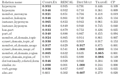
Table 5 shows the filtered MRR for the reimplemented models and each relation of WN18, confirming the advantage of ComplEx on antisymmetric relations while losing
nothing on the others. 2D projections of the relation embeddings (Figures 8 & 9) visually corroborate the results.
On FB15K, the gap is much more pronounced and theComplExmodel largely
outper-formsHolE, with a filtered MRR of 0.692 and 59.9% of Hits at 1, compared to 0.524 and
40.2% forHolE. This difference of scores between the two models, though they have been
proved to be equivalent (Hayashi and Shimbo, 2017), is due to the use of the aforementioned max-margin loss in the originalHolEpublication (Nickel et al., 2016b) that performs worse
than the log-likelihood on this dataset, and to the generation of more than one negative sample per positive in these experiments. This has been confirmed and discussed in details by Trouillon and Nickel (2017). The fact that DistMult yields fairly high scores (0.654
Relation name ComplEx RESCAL DistMult TransE CP
hypernym 0.953 0.935 0.791 0.446 0.109
hyponym 0.946 0.932 0.710 0.361 0.009
member meronym 0.921 0.851 0.704 0.418 0.019 member holonym 0.946 0.861 0.740 0.465 0.134 instance hypernym 0.965 0.833 0.943 0.961 0.233 instance hyponym 0.945 0.849 0.940 0.745 0.040
has part 0.933 0.879 0.753 0.426 0.035
part of 0.940 0.888 0.867 0.455 0.094
member of domain topic 0.924 0.865 0.914 0.861 0.007 synset domain topic of 0.930 0.855 0.919 0.917 0.153 member of domain usage 0.917 0.629 0.917 0.875 0.001 synset domain usage of 1.000 0.541 1.000 1.000 0.134 member of domain region 0.865 0.632 0.635 0.865 0.001 synset domain region of 0.919 0.655 0.888 0.986 0.149 derivationally related form 0.946 0.928 0.940 0.384 0.100 similar to 1.000 0.001 1.000 0.244 0.000 verb group 0.936 0.857 0.897 0.323 0.035
also see 0.603 0.302 0.607 0.279 0.020
Table 5: Filtered Mean Reciprocal Rank (MRR) for the models tested on each relation of the WordNet data set (WN18).
to be false—for antisymmetric relations—and largely impacts the average precision of the
DistMultmodel (Figure 4).
RESCAL, that represents each relation with aK×Kmatrix, performs well on WN18 as there are few relations and hence not so many parameters. On FB15K though, it probably overfits due to the large number of relations and thus the large number of parameters to learn, and performs worse than a less expressive model likeDistMult. On both data sets,
TransEand CP are largely left behind. This illustrates again the power of the multilinear
product in the first case, and the importance of learning unique entity embeddings in the second. CP performs especially poorly on WN18 due to the small number of relations, which magnifies this subject/object difference.
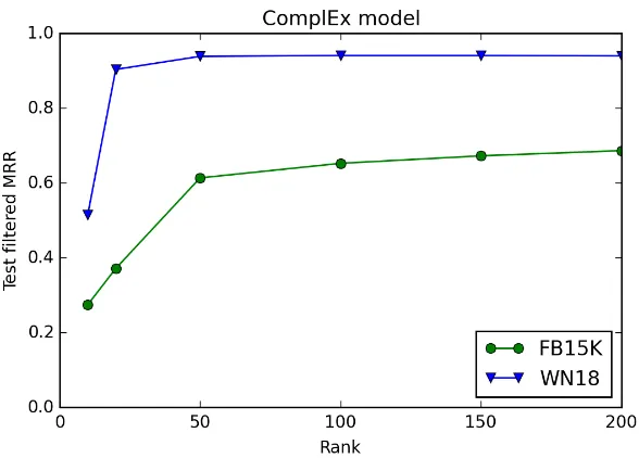
Figure 5 shows that the filtered MRR of theComplExmodel quickly converges on both
data sets, showing that the low-rank hypothesis is reasonable in practice. The little gain of performances for ranks comprised between 50 and 200 also shows thatComplEx does not
perform better because it has twice as many parameters for the same rank—the real and imaginary parts—compared to other linear space complexity models but indeed thanks to its better expressiveness.
Figure 5: Best filtered MRR forComplExon the FB15K and WN18 data sets for different
ranks. Increasing the rank gives little performance gain for ranks of 50−200.
much on WN18. We think this may also explain the large gap of improvement ComplEx
provides on this data set compared to previously published results—as DistMultresults
are also better than those previously reported (Yang et al., 2015)—along with the use of the log-likelihood objective. It seems that in general AdaGrad is relatively insensitive to the initial learning rate, perhaps causing some overconfidence in its ability to tune the step size online and consequently leading to less efforts when selecting the initial step size.
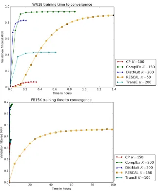
5.4 Training time
As defended in Section 2, having a linear time and space complexity becomes critical when the dataset grows. To illustrate this, we report in Figure 6 the evolution of the filtered MRR on the validation set as a function of time, for the best set of validated hyper-parameters for each model. The convergence criterion used is the decrease of the validation filtered MRR—computed every 50 iterations—with a maximum number of iterations of 1000 (see Algorithm 1). All models have a linear complexity except for RESCAL that has a quadratic one in the rank of the decomposition, as it learns one matrix embedding for each relation
r∈ R. Timings are measured on a single NVIDIA Tesla P40 GPU.
Figure 6: Evolution of the filtered MRR on the validation set as a function of time, on WN18 (top) and FB15K (bottom) for each model for its best set of hyper-parameters. The best rank K is reported in legend. Final black marker indicates that the maximum number of iterations (1000) has been reached (RESCAL on WN18,
TransEon FB15K).
a much higher memory footprint, which implies more processor cache misses due to the uniformly-random nature of the SGD sampling.
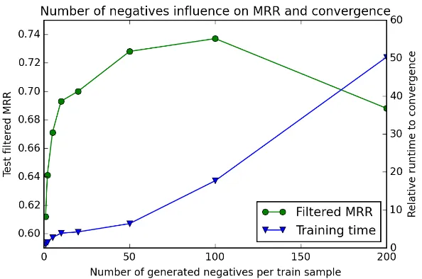
Figure 7: Influence of the number of negative triples generated per positive training example on the filtered test MRR and on training time to convergence on FB15K for the
ComplExmodel withK = 200,λ= 0.01 andα= 0.5. Times are given relative to
the training time with one negative triple generated per positive training sample (= 1 on time scale).
5.4.1 Influence of Negative Samples
We further investigated the influence of the number of negatives generated per positive training sample. In the previous experiment, due to computational limitations, the number of negatives per training sample, η, was validated over the set {1,2,5,10}. On WN18 it proved to be of no help to have more than one generated negative per positive. Here we explore in which proportions increasing the number of generated negatives leads to better results on FB15K. To do so, we fixed the best validatedλ, K, αobtained from the previous experiment. We then letη vary in{1,2,5,10,20,50,100,200}.
Figure 7 shows the influence of the number of generated negatives per positive train-ing triple on the performance of ComplEx on FB15K. Generating more negatives clearly
improves the results up to 100 negative triples, with a filtered MRR of 0.737 and 64.8% of Hits@1, before decreasing again with 200 negatives, probably due to the too large class imbalance. The model also converges with fewer epochs, which compensates partially for the additional training time per epoch, up to 50 negatives. It then grows linearly as the number of negatives increases.
5.4.2 WN18 Embeddings Visualization
We used principal component analysis (PCA) to visualize embeddings of the relations of the WordNet data set (WN18). We plotted the four first components of the best DistMult
andComplEx model’s embeddings in Figures 8 & 9. For theComplExmodel, we simply
Figure 8: Plots of the first and second components of the WN18 relations embeddings using principal component analysis. Red arrows link the labels to their point. Top:
ComplEx embeddings. Bottom: DistMult embeddings. Opposite relations
Figure 9: Plots of the third and fourth components of the WN18 relations embeddings using principal component analysis. Red arrows link the labels to their point. Top:
ComplEx embeddings. Bottom: DistMult embeddings. Opposite relations
Most of WN18 relations describe hierarchies, and are thus antisymmetric. Each of these hierarchic relations has its inverse relation in the data set. For example: hypernym/ hyponym,part of/has part,synset domain topic of/member of domain topic. Since
DistMult is unable to model antisymmetry, it will correctly represent the nature of each
pair of opposite relations, but not the direction of the relations. Loosely speaking, in the hypernym / hyponym pair the nature is sharing semantics, and the direction is that one entity generalizes the semantics of the other. This makes DistMultrepresenting the
opposite relations with very close embeddings. It is especially striking for the third and fourth principal component (Figure 9). Conversely,ComplExmanages to oppose spatially
the opposite relations.
6. Related Work
We first discuss related work about complex-valued matrix and tensor decompositions, and then review other approaches for knowledge graph completion.
6.1 Complex Numbers
When factorization methods are applied, the representation of the decomposition is gen-erally chosen in accordance with the data, despite the fact that most real square matrices only have eigenvalues in the complex domain. Indeed in the machine learning community, the data is usually real-valued, and thus eigendecomposition is used for symmetric matri-ces, or other decompositions such as (real-valued) singular value decomposition (Beltrami, 1873), non-negative matrix factorization (Paatero and Tapper, 1994), or canonical polyadic decomposition when it comes to tensors (Hitchcock, 1927).
Conversely, in signal processing, data is often complex-valued (Stoica and Moses, 2005) and the complex-valued counterparts of these decompositions are then used. Joint diago-nalization is also a much more common tool than in machine learning for decomposing sets of (complex) dense square matrices (Belouchrani et al., 1997; De Lathauwer et al., 2001).
Some works on recommender systems use complex numbers as an encoding facility, to merge two real-valued relations, similarity and liking, into one single complex-valued matrix which is then decomposed with complex embeddings (Kunegis et al., 2012; Xie et al., 2015). Still, unlike our work, it is not real data that is decomposed in the complex domain.
In deep learning, Danihelka et al. (2016) proposed an LSTM extended with an associative memory based on complex-valued vectors for memorization tasks, and Hu et al. (2016) a complex-valued neural network for speech synthesis. In both cases again, the data is first encoded in complex vectors that are then fed into the network.
Conversely to these contributions, this work suggests that processing real-valued data with complex-valued representation, through a projection onto the real-valued subspace, can be a very simple way of increasing the expressiveness of the model considered.
6.2 Knowledge Graph Completion
et al., 2008) and the Google Knowledge Vault (Dong et al., 2014). Motivating applications of knowledge graph completion include question answering (Bordes et al., 2014b) and more generally probabilistic querying of knowledge bases (Huang and Liu, 2009; Krompaß et al., 2014).
First approaches to relational learning relied upon probabilistic graphical models (Getoor and Taskar, 2007), such as bayesian networks (Friedman et al., 1999) and markov logic net-works (Richardson and Domingos, 2006; Raedt et al., 2016).
With the first embedding models, asymmetry of relations was quickly seen as a problem and asymmetric extensions of tensors were studied, mostly by either considering indepen-dent embeddings (Franz et al., 2009) or considering relations as matrices instead of vectors in the RESCAL model (Nickel et al., 2011), or both (Sutskever, 2009). Direct extensions were based on uni-,bi- and trigram latent factors for triple data (Garcia-Duran et al., 2016), as well as a low-rank relation matrix (Jenatton et al., 2012). Bordes et al. (2014a) propose a two-layer model where subject and object embeddings are first separately combined with the relation embedding, then each intermediate representation is combined into the final score.
Pairwise interaction models were also considered to improve prediction performances. For example, the Universal Schema approach (Riedel et al., 2013) factorizes a 2D unfolding of the tensor (a matrix of entity pairs vs. relations) while Welbl et al. (2016) extend this also to other pairs. Riedel et al. (2013) also consider augmenting the knowledge graph facts by exctracting them from textual data, as does Toutanova et al. (2015). Injecting prior knowledge in the form of Horn clauses in the objective loss of the Universal Schema model has also been considered (Rocktaschel et al., 2015). Chang et al. (2014) enhance the RESCAL model to take into account information about the entity types. For recommender systems (thus with different subject/object sets of entities), Baruch (2014) proposed a non-commutative extension of the CP decomposition model. More recently, Gaifman models that learn neighborhood embeddings of local structures in the knowledge graph showed competitive performances (Niepert, 2016).
In the Neural Tensor Network (NTN) model, Socher et al. (2013) combine linear trans-formations and multiple bilinear forms of subject and object embeddings to jointly feed them into a nonlinear neural layer. Its non-linearity and multiple ways of including in-teractions between embeddings gives it an advantage in expressiveness over models with simpler scoring function likeDistMultor RESCAL. As a downside, its very large number of parameters can make the NTN model harder to train and overfit more easily.
The original multilinear DistMultmodel is symmetric in subject and object for every
relation (Yang et al., 2015) and achieves good performance on FB15K and WN18 data sets. However it is likely due to the absence of true negatives in these data sets, as discussed in Section 5.3.2.
TheTransEmodel from Bordes et al. (2013b) also embeds entities and relations in the
same space and imposes a geometrical structural bias into the model: the subject entity vector should be close to the object entity vector once translated by the relation vector.
A recent novel way to handle antisymmetry is via the Holographic Embeddings (HolE)
model by Nickel et al. (2016b). In HolE the circular correlation is used for combining
shifts. This model has been shown to be equivalent to the ComplExmodel (Hayashi and
Shimbo, 2017; Trouillon and Nickel, 2017).
7. Discussion and Future Work
Though the decomposition proposed in this paper is clearly not unique, it is able to learn meaningful representations. Still, characterizing all possible unitary diagonalizations that preserve the real part is an interesting open question. Especially in an approximation setting with a constrained rank, in order to characterize the decompositions that minimize a given reconstruction error. That might allow the creation of an iterative algorithm similar to eigendecomposition iterative methods (Saad, 1992) for computing such a decomposition for any given real square matrix.
The proposed decomposition could also find applications in many other asymmetric square matrices decompositions applications, such as spectral graph theory for directed graphs (Cvetkovi´c et al., 1997), but also factorization of asymmetric measures matrices such as asymmetric distance matrices (Mao and Saul, 2004) and asymmetric similarity matrices (Pirasteh et al., 2015).
From an optimization point of view, the objective function (Equation (10)) is clearly non-convex, and we could indeed not be reaching a globally optimal decomposition using stochastic gradient descent. Recent results show that there are no spurious local minima in the completion problem of positive semi-definite matrix (Ge et al., 2016; Bhojanapalli et al., 2016). Studying the extensibility of these results to our decomposition is another possible line of future work. The first step would be generalizing these results to symmetric real-valued matrix completion, then generalization to normal matrices should be straight-forward. The two last steps would be extending to matrices that are expressed as real part of normal matrices, and finally to the joint decomposition of such matrices as a tensor. We indeed noticed a remarkable stability of the scores across different random initialization of
ComplExfor the same hyper-parameters, which suggests the possibility of such theoretical
property.
Practically, an obvious extension is to merge our approach with known extensions to tensor factorization models in order to further improve predictive performance. For ex-ample, the use of pairwise embeddings (Riedel et al., 2013; Welbl et al., 2016) together with complex numbers might lead to improved results in many situations that involve non-compositionality. Adding bigram embeddings to the objective could also improve the results as shown on other models (Garcia-Duran et al., 2016). Another direction would be to develop a more intelligent negative sampling procedure, to generate more informative negatives with respect to the positive sample from which they have been sampled. This would reduce the number of negatives required to reach good performance, thus accelerat-ing trainaccelerat-ing time. Extension to relations between more than two entities, n-tuples, is not straightforward, asComplEx’s expressiveness comes from the complex conjugation of the
8. Conclusion
We described a new matrix and tensor decomposition with complex-valued latent factors called ComplEx. The decomposition exists for all real square matrices, expressed as the
real part of normal matrices. The result extends to sets of real square matrices—tensors— and answers to the requirements of the knowledge graph completion task : handling a large variety of different relations including antisymmetric and asymmetric ones, while being scalable. Experiments confirm its theoretical versatility, as it substantially improves over the state-of-the-art on real knowledge graphs. It shows that real world relations can be efficiently approximated as the real part of low-rank normal matrices. The generality of the theoretical results and the effectiveness of the experimental ones motivate for the application to other real square matrices factorization problems. More generally, we hope that this paper will stimulate the use of complex linear algebra in the machine learning community, even and especially for processing real-valued data.
Acknowledgments
This work was supported in part by the Association Nationale de la Recherche et de la Tech-nologie through the CIFRE grant 2014/0121, in part by the Paul Allen Foundation through an Allen Distinguished Investigator grant, and in part by a Google Focused Research Award. We would like to thank Ariadna Quattoni, St´ephane Clinchant, Jean-Marc Andr´eoli, Sofia Michel, Alejandro Blumentals, L´eo Hubert and Pierre Comon for their helpful comments and feedback.
References
Noga Alon, Shay Moran, and Amir Yehudayoff. Sign rank versus vc dimension. In Confer-ence on Learning Theory, pages 47–80, 2016.
Sren Auer, Christian Bizer, Georgi Kobilarov, Jens Lehmann, and Zachary Ives. DBpedia: A nucleus for a web of open data. In International Semantic Web Conference, Busan, Korea, pages 11–15. Springer, 2007.
Guy Baruch. A ternary non-commutative latent factor model for scalable three-way real tensor completion. arXiv preprint arXiv:1410.7383, 2014.
Adel Belouchrani, Karim Abed-Meraim, J-F Cardoso, and Eric Moulines. A blind source separation technique using second-order statistics. IEEE Transactions on Signal Process-ing, 45(2):434–444, 1997.
Eugenio Beltrami. Sulle funzioni bilineari. Giornale di Matematiche ad Uso degli Studenti Delle Universita, 11(2):98–106, 1873.