190
Copyright © 2011-15. Vandana Publications. All Rights Reserved.
Volume-5, Issue-2, April-2015
International Journal of Engineering and Management Research
Page Number: 190-196
Data Mining Approach for Estimation of Earthquake Hazard in Shillong
Region
Manisha Singh1, Radhakrishnan Rambola2
1
Master of Technology Student, Department of Computing Science and Engineering, Galgotias University, Greater Noida, Uttar Pradesh, INDIA
2
Associate Professor, Department of Computing Science and Engineering, Galgotias University, Greater Noida, Uttar Pradesh, INDIA
ABSTRACT
North India is one of the earthquake active zone in Indian subcontinent. In this area, a series of medium to large magnitude earthquake can be seen. The expected earthquake of intensity up to IX can be observed. Therefore, for reducing the loss of life and property, it is important to analyze the earthquake risk in the considered region, properly. In this paper data mining approach have been applied .This paper contains the calculation of the largest annual earthquake magnitude, its probability of occurrence and the return period of largest earthquake for the earthquake prone Shillong region of North East India using Gumbel’s type I distribution which is based on the extreme value theory has been estimated. Most probable annual maxima have also been calculated for the considered region. The line of expected extreme which is based on 46 years (1963-2008) of seismicity data of yearly extreme values of earthquakes for the region have been plotted. The medium to large size earthquakes which is expected to occur in this region has been predicted.
Keywords— Gumble’s Theory, Line of expected stream MM intensity.
I.
INTRODUCTION
To analyze the seismic risk has been a major problem for earthquake engineering. Time of occurrence of earthquake, location and magnitude of future earthquake cannot be predicted precisely because of incomplete understanding of geophysical phenomenon and present infrastructure available. Many statistical approaches have been proposed for the estimation of occurrence of largest
earthquake (Kaila et al., 1972; Yegulap and kuo 1974; Lomnitz, 1974; Shanker and Singh, 1997; Papazachos, 1989). These statistical methods are being used for risk analysis and probability estimation.
Extreme value theory given by Gumbel (1958) has been used by number of researchers for earthquake predictions of different region of the world. In this study calculations based on this model have been carried out for estimating the largest annual earthquake, its return period, and annual maxima in the Shillong region.
II.
METHODOLOGY
The methodology used in this approach is Gumbel’s Type I Distribution. Initially, the Gumbel’s theory was proposed for the estimation of flood data analysis and now being frequently used for the earthquake data. It is based on the Poisson random variable function. The shape of Gumble model does not depends on the distribution parameters. It is a probability model which gives an adequate basis for making predictions concerning the occurrence of largest annual earthquake magnitudes. This theory requires p independent observations which are collected continuously from long years. This should be divisible into N data sets each having extremes (N). The largest magnitude from each earthquake data must be taken and should be arranged in ascending order of their magnitude i.e. m1 < m2 <m3….<mp. Where p=N denotes
total no of intervals of the data sets. The frequency of each (mk) in the order set of extremes is represented as
G (mk) = k/N+1 (1)
Where K is the rank for each mk
191
Copyright © 2011-15. Vandana Publications. All Rights Reserved.
From this assumptions it follows that m (m), largest annual earthquake magnitude, is distributed with cumulative distribution function G (m).This model is given by Epstein and Lomnitz (1966) for the occurrence of largest earthquake.
The Cumulative distribution function (2) is called the “Gumbel type I” distribution of largest value. The
parameter α and β are the average number of earthquake with magnitude greater than >0 per year, β is the inverse of
the average magnitude of earthquake for the shillong region and e (m) is the maximum annual earthquake magnitude. The parameter α and β found from the least square fit to the equation
ln [-ln G (m)] = ln α-βm (3) Equation (3) is the derivation of equation (2)
β is considered a measure of concentration about the
mode. The table 2 defines the estimation of parameters α
and β.
The return period of earthquake of magnitude m is given by
Tm=1/Nm (4)
Where Nm= αe-βm is the number of expected earthquake per
year exceeding magnitude m.
Tm is also called average reoccurrence period of
earthquake. Table 3 defines the average recurrence period for the given earthquakes within shillong region.
Earthquake Hazard Ht (m) is the probability of
reoccurrence of an earthquake of magnitude m within a period of T years is given by
Ht (m) =1-exp (-αTe-βm
Association Rule Mining: Association rule mining discovers interesting correlations among database attributes (Agrawal et al., 1993). Association rules are in the form of implications
) (5)
β→ parameter, slope of mean line of expected extreme
(LEE)
α→ Parameter inter-related to β (intercept) m→ Magnitude
k→ serial number k=1,2,3...., n
p→ number of independent collected observation G (m)→ relative frequency( Probability)
N→ Sample size
Nm→ Mean expected number of events Tm→ Mean return period
III.
PRIOR APPROACH
⇒
P Q[s, c ] , P
⊂
M, Q⊂
Mwhere P, B and M are sets of items (i.e., attributes), classified by two measures: su p p o r t (s) and
c o n f i d e n c e (c). The support of a rule P
⇒
Q defines the probability that a database event contains both P and Q, whereas the confidence of the rule defines the conditional probability that a database event containing P also contains Q.For an example, if we apply association rule on seismological data then it would be of the following type
L o c ati o n in L ^ d e p th ≥ 100 Km
⇒
mag n i tu d e ≥ 5R [1%, 50%] which is express as follows: whenever an earthquake occurs in location
L at a depth of over 100Km its magnitude is likely to be greater than 5R with a probability of 50%; this combination occurred in 1% of all recorded events.
In case of temporal association rule mining (se qu e n c i n g), which detects correlations between events with time as in the following example: Ar e a i n
Al ^ m ag n i tu d e ≥ 7R
⇒
Ar e a in A2 within [0,30 days] [0.1%, 30%]
Which is express as follows: whenever an
earthquake occurs in area A1 with a magnitude
greater than 7R it is likely that another earthquake occurs in area A2 within a month after
the first event with a probability of 30%; this combination occurred in 0.1% of all recorded events.
By identifying and analyzing event sequences
( se i smi c se qu e n c e s) seismologists can be aid in studying this type of earthquake behavior.
192
Copyright © 2011-15. Vandana Publications. All Rights Reserved.
Figure 1. Discovering cluster of earthquake epicentre (Theodoridis, 2003)
Various clustering approaches have been pro-posed in the literature. Local spatial-temporal clusters of low magnitude events can be extracted (Dzwinel et al., 2003) using multi-dimensional correlations .Correlations between the clusters and the earthquakes are also recognized. In case of multidimensional Signal (Sheikholeslami et al., 2000) for spatial data, processing techniques can be applied. A clustering method associated with wavelet transform can identify clusters by finding dense regions in the transformed data. Finally, hybrid methodologies have been proposed (Guo et al., 2003) where spatial clustering is combined with high-dimensional clustering.
Classification of Data: Data classification is one of the most common supervised learning techniques. Its first objective is to analyze a (labeled) training set and, with the help of this procedure, build a model for labeling new data entries (Han & Kamber, 2000). A classification model is built in first step using a t r a i n i n g d a t a
s e t
For the example, the (hypothetical) decision tree illustrated in Figure 2 tries to “predict” the macro seismic
intensity at a site given the depth and the magnitude of an earthquake, the geographic area and the local geology. Such implication uncovers correlations between the attributes of the seismological database and decision trees. Such a type is already used by local authorities to process actions for response and relief of the population after a strong earthquake.
consisting of database records which are associated with certain class and a proper supervised learning method, e.g. decision trees or neural networks. For decision trees, the model consists of a tree of “if” statements focal to a label which denote the record of the class it belongs. In the second step, the built model which is not included in the training set is used for the classification of records. Several methods have been developed for classification, including decision tree induction, neural networks and Bayesian networks (Fayad et al., 1996).
Geography
Depth
Magnitude Geology
Intensity<V Intensity>=V Magnitude
Intensity>III
Intensity<IV Intensity>=V Hellenic arc
<60km >=60km
<6 >=6 soil rock
<6 >=6
Figure 2. An example of decision tree for seismicity data
IV. OUR APPROACH
Regression Analysis: The approach used here is statistical approach of linear regression. For implementation of this model, data form earthquake database was used, making a previous error data by perceptive the string data. For the best results which are obtained in the tests, data sets (numerical) were created, that generate a pattern relevant to this data. Some important relationship between variables are identified: magnitude calculation based on their latitude and longitude, number of death according to the earthquake magnitude, injuries per year, daily losses, losses per year and depth according to the length.
The graph between reduced statistics and design magnitude shows the equation of linear regression which is same likeGutenberg and Richter (1956)
LogN= a-b (m) (6) Where a, b is a regression coefficient.
V. DATA USED
193
Copyright © 2011-15. Vandana Publications. All Rights Reserved.
and their adjoining region and the table gives the calculation of largest annual earthquake magnitude.
Figure 3: Seismicity of northeast India region (Singh et al., 2005). The structural features and the four major tectonic zones (I–IV) are also shown. Zone III, Shilong region has been taken for the present study.
The data given in table 1 is the data for the sillong region i.e for Zone III for which have calculated the frequency of the earthquake, its return period and the probability of the occurrence.
Fig 4. Graph between maximum magnitude and reduced statistics showing regression analysis equation
TABLE 1: Calculation for Gumbel's Annual Maximum Distribution & Estimation of α and β.
Here are the graphs for the Gumbel’s equation of table 1
for the estimation of α and β.
Y=-3.384x+16.13 this is called gumbel’s equation which is same as regression analysis equation.
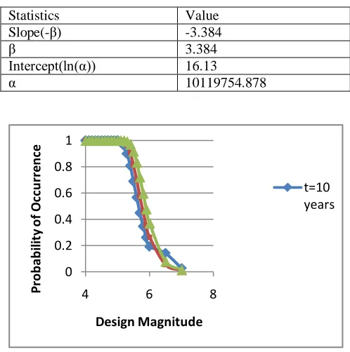
Table 2. Estimated Gumbel’s Parameters α and β
Statistics Value Slope(-β) -3.384
β 3.384
Intercept(ln(α)) 16.13
α 10119754.878
Fig 5. Graph showing Probability of occurrence with design magnitude for t= 10, 20, 30 years
y = -3.384x + 16.13 R² = 0.971
-5 -4 -3 -2 -1 0 1 2
4 4.5 5 5.5 6
Re
duc
ed S
ta
tis
tic
ln
(-l
n(
G
(m
))=
ln
α
-β
M
Maximum Magnitude
0 0.2 0.4 0.6 0.8 1
4 6 8
Pr
ob
ab
ili
ty
of
O
ccu
rr
en
ce
Design Magnitude
194
Copyright © 2011-15. Vandana Publications. All Rights Reserved.
Table3. Predicted Annual number of earthquakes and its return period
Table 4: Most probable largest earthquake hazard Ht (m)
for Different Magnitude and Time Periods (t=10, 20, 30) years
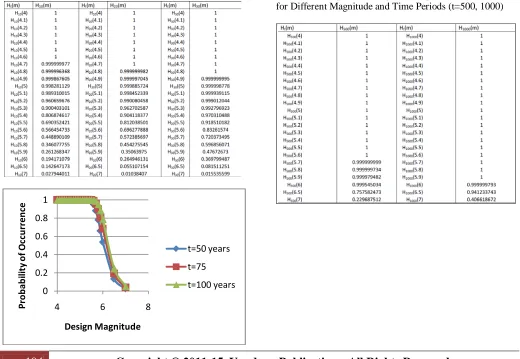
Fig 6. Graph showing Probability of occurrence with design magnitude for t= 50, 75, 100 years
Table 5: Most probable largest earthquake hazard Ht
Table 6: Most probable largest earthquake hazard H (m) for Different Magnitude and Time Periods (t=50,75, 100) years
t (m)
for Different Magnitude and Time Periods (t=500, 1000)
0 0.2 0.4 0.6 0.8 1
4 6 8
Pr
ob
ab
ili
ty
of
O
ccu
rr
en
ce
Design Magnitude
195
Copyright © 2011-15. Vandana Publications. All Rights Reserved.
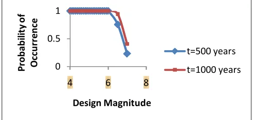
Fig 7. Graph showing probability of occurrence with design magnitude for t= 500, 1000 years
For an earthquake of magnitude 6, which has a return period of 64.97 years, the 89% probability reccurrence period is calculated as and reported in Table 7. T89 = -Tm
Magnitude(m) ln (1-0.89)
T
able 7. Recurrence Period with 89% probabilityReturn Period (years)
Recurrence period (years)
5 5.5 5.8 6 6.5 7
2.2 11.96 33.02 64.97 352.83 1916.01
4.856004809 26.39900796 72.88421763 143.4066511 778.7928076 4229.160806
VI. DISCUSSION AND CONCLUSION
A most important utility of this work is to express the usefulness and authenticity of extreme value theory when applied to the estimation of earthquake occurrence. Seismic threat and related earthquake engineering purposes usually require evaluation of return periods or probabilities of exceedance of specific levels of design load criteria or extremal safety conditions. The seismicity of the North east India region displays significant change in magnitude and frequency of earthquake in space and time. This study advocates that the region is one of the most earthquake active regions. The present technique uses 46 years of seismicity data to analyses the largest annual earthquake magnitude. The Gumbel’s extreme value method proved very useful to estimate the future earthquake occurrences for the civil and scientific uses. It has attracted the attention of seismologist for regional
seismicity variation and earthquake engineers for civil protection. Tables 1 and 3 shows the probability of occurrence and return periods for different magnitude and time periods.
The merit of the analysis over other statistical techniques lies in the fact that one can forecast the mean return period of different magnitudes over several years. Here the return periods for magnitude 6 earthquake have been estimated to be 64.97 years. However, general interpretation of 89% probability recurrence period result is that, within the Shillong region, there is 89% probability that, in any given 143.41 years periods, at least one earthquake of magnitude 6.0 or greater will occur (Table 7). The earthquake hazard parameters for the considered region have been reported in Table (4, 5 and 6) for different magnitudes over 10, 20, 30, 50, 75, 100, 500, 1000 years duration. This table illustrates that risk value decreases with increasing magnitudes. Probability curves (Figures 5, 6 and 7) indicates that there is non-zero probability no event occurring over any given period of time, since probability of any particular event never reaches 1.0. For example, the probability of an earthquake of 6.0 occurring in Shillong area within any 500 years, is 0.999 and for 6.5 in 1000 years (Figure 7). It means, it is certain that at least one such event will occur within that period of time.
In all statistical analyses generally, a huge amount of seismicity data is required to derive return periods. Although, the present analysis uses 46-years of data to estimate the seismic risk and return period, however, the analysis may be considered to be reliable, since the value
of the parameters lnα and β (Table 8) which are used in estimating the return periods and risk do not change much for the use of short or long duration of seismicity data. Thus the estimates offered in this study may permit certain consideration for civil engineering constructions.
This paper analyses that regression analysis (Figure 4) performs well in comparison to other data mining techniques. To improve the performance of regression analysis, other statistical based features linear regression can be subsumed.
0 0.5 1
4 6 8
Pr
ob
ab
ili
ty
o
f
O
ccu
rr
en
ce
Design Magnitude
t=500 years t=1000 years
Table 8. Earthquake hazard parameters for shillong Region
Most probable lnα n β
annual maxima
196
Copyright © 2011-15. Vandana Publications. All Rights Reserved.
VII.
A
CKNOWLEDGMENTThe authors would like to express his sincere thanks to all authors’ whose references and research works helped us a lot for the preparation of this manuscript.
REFERENCES
[1] Agarwal, S., Agrawal, R., Deshpande, P., Gupta, A., Naughton, J., Ramakrishnan, R., et al. (1996). On the computation of multidimensional aggregates. In Proceedings of the 22nd International Conference on Very Large Databases, VLDB’96, Bombay, India.
[2] Kaufman, L. & Rousseeuw, P. (1990). Finding Groups in Data: An Introduction to Cluster Analysis. John Wiley & Sons.
[3] Dzwinel, W., Yuen, D., Kaneko, Y, Boryczko, K., & Ben-Zion, Y (2003). Multi-resolution clustering analysis and 3-D visualization of multitudinous synthetic earthquakes. Visual Geosciences, 8(1), 12-25.
[4] Sheikholeslami, G., Chatterjee, S., & Zhang, A. (2000). WaveCluster: A Wavelet-based Clustering Approach for Spatial Data in Very Large Databases. The VLDB Journal, 8(3-4), 289-304.
[5] Guo, D., Peuquet D., & Gahegan, M. (2003). ICE- AGE. Interactive clustering and exploration of large and high- Dimensional geodata. Geolnformatica, 7(3), 229-253.
[6] Han, J., & Kamber, M. (2000). Data mining: Concepts and techniques. Morgan Kaufmann.
[7] Fayad, U., Piatetsky-Shapiro, G., Smith, P., & Uthuru- sami, R. (1996). Advances in Knowledge Discovery and Data Mining. MIT Press
[8] Koperski K., & Han J. (1995). Discovery of spatial
as-sociation rules in geographic information databases. In Proceedings of the 4th International Symposium on Large in Spatial Databases, SSD’95, Portland, MA, USA.
[9] Stefanovic, N., Han, J., & Koperski, K. (2000). Object-based selective materialization for efficient implementation of spatial data cubes. IEEE Transactions on Knowledge and Data Engineering, 12(6), 938-958. [10] Yegulap T M, Kuo J T 1974: Bull. Seismol. Soc. Am., 64, 393-414
[11] Shanker D, Singh V P, Singh H N 1995: Acta Geod. Geoph. Hung., 30, 379 395.
[12] Rao P S, Rao B R 1979: Mausam, 30, 2/3, 267-273. [13] Shanker D, Singh V P 1997: Proc. Indian Natn. Sci. Acad., 63, A, 2, 71-76.
[14] Tipnis R S, Srivastava L S 1968: Bull. Ind. Soc. Earthquake Tech., 5, 107-118.
[15] Powell J A, Duda S J 1975: Pure and Appl. Geophys.
[16] Papazachos B C 1989:
113, 444-460.
Bull. Seismol. Soc. Am.,
[17] Epstein B, Lomnitz C 1966:
79, 77-84.
Nature [18] Kaila K L, Gaur V K, Narain H 1972:
, 211, 954-956. Dull. Seismol. Soc. Am.,
[19] Karnik V, Hiibnerova Z 1968: 62, 1119-1132.
Pure and Appl. Geophys., 70, 61-73.