More Efficient Estimation for Logistic Regression with
Optimal Subsamples
HaiYing Wang [email protected]
Department of Statistics University of Connecticut Storrs, CT 06269, USA
Editor:Tong Zhang
Abstract
In this paper, we propose improved estimation method for logistic regression based on sub-samples taken according the optimal subsampling probabilities developed in Wang et al. (2018). Both asymptotic results and numerical results show that the new estimator has a higher estimation efficiency. We also develop a new algorithm based on Poisson sub-sampling, which does not require to approximate the optimal subsampling probabilities all at once. This is computationally advantageous when available random-access memory is not enough to hold the full data. Interestingly, asymptotic distributions also show that Poisson subsampling produces a more efficient estimator if the sampling ratio, the ratio of the subsample size to the full data sample size, does not converge to zero. We also obtain the unconditional asymptotic distribution for the estimator based on Poisson subsampling. Pilot estimators are required to calculate subsampling probabilities and to correct biases in un-weighted estimators; interestingly, even if pilot estimators are inconsistent, the proposed method still produce consistent and asymptotically normal estimators.
Keywords: Asymptotic Distribution, Logistic Regression, Massive Data, Optimal Sub-sampling, Poisson Sampling.
1. Introduction
Extraordinary amounts of data that are collected offer unparalleled opportunities for ad-vancing complicated scientific problems. However, the incredible sizes of big data bring new challenges for data analysis. A major challenge of big data analysis lies with the thirst for computing resources. Faced with this, subsampling has been widely used to reduce the computational burden, in which intended calculations are carried out on a subsample that is drawn from the full data, see Drineas et al. (2006a,b,c); Mahoney and Drineas (2009); Drineas et al. (2011); Mahoney (2011); Halko et al. (2011); Clarkson and Woodruff (2013); Kleiner et al. (2014); McWilliams et al. (2014); Yang et al. (2017), among others.
A key to success of a subsampling method is to specify nonuniform sampling probabil-ities so that more informative data points are sampled with higher probabilprobabil-ities. For this purpose, normalized statistical leverage scores or its variants are often used as subsampling probabilities in the context of linear regression, and this approach is termed algorithmic leveraging (Ma et al., 2015). It has demonstrated remarkable performance in better using of a fixed amount of computing power (Avron et al., 2010; Meng et al., 2014). Statistical leverage scores only contain information in the covariates and do not take into account
c
the information contained in the observed responses. Wang et al. (2018) derived optimal subsampling probabilities that minimize the asymptotic mean squared error (MSE) of the subsampling-based estimator in the context of logistic regression. The optimal subsam-pling probabilities directly depend on both the covariates and the responses to take more informative subsamples. Wang et al. (2018) used a inverse probability weighted estimator based on the optimal subsample, where more informative data points are assigned smaller weights in the objective function. Thus, we can improve the estimation efficiency based on the optimal subsample by using a better weighting scheme.
In this paper, we propose more efficient estimators based on subsamples taken randomly according to the optimal subsampling probabilities. We will derive asymptotic distributions to show that asymptotic variance-covariance matrices of the new estimators are smaller, in Loewner ordering, than that of the weighted estimator in Wang et al. (2018). We also consider to use Poisson subsampling. Asymptotic distributions show that Poisson subsam-pling is more efficient in parameter estimation when the subsample size is proportional to the full data sample size. It is also computationally beneficial to use Poisson subsampling because there is no need to calculate and use subsampling probabilities for all data points simultaneously.
Before presenting the framework of the paper, we give a brief review of the emerging field of subsampling-based methods. For linear regression, Drineas et al. (2006d) developed a subsampling method and focused on finding influential data units for the least squares (LS) estimates. Drineas et al. (2011) developed an algorithm by processing the data with randomized Hadamard transform and then using uniform subsampling to approximate LS estimates. Drineas et al. (2012) developed an algorithm to approximate statistical leverage scores that are used for algorithmic leveraging. Yang et al. (2015) showed that using nor-malized square roots of statistical leverage scores as subsampling probabilities yields better approximation than using original statistical leverage scores, if they are very nonuniform. The aforementioned studies focused on developing algorithms for fast approximation of LS estimates. Ma et al. (2015) considered the statistical properties of algorithmic leveraging. They derived biases and variances of leverage-based subsampling estimators in linear regres-sion and proposed a shrinkage algorithmic leveraging method to improve the performance. Raskutti and Mahoney (2016) considered both the algorithmic and statistical aspects of solving large-scale LS problems using random sketching. Wang et al. (2019) and Wang (2019) developed an information-based optimal subdata selection method to select subsam-ple deterministically for ordinary LS in linear regression. The aforesaid results were obtained exclusively within the context of linear models. Fithian and Hastie (2014) proposed a com-putationally efficient local case-control subsampling method for logistic regression with large imbalanced data. Han et al. (2019) developed a local uncertainty sampling approach for multi-class logistic regression. Recently, Wang et al. (2018) developed an Optimal Subsam-pling Method under the A-optimality Criterion (OSMAC) for logistic regression; Yao and Wang (2019) and Ai et al. (2019) extended this method to include multi-class logistic regres-sion and generalized linear regresregres-sion models, respectively. Although they derived optimal subsampling probabilities, they did not investigate whether a better weighting scheme can further improve the estimation efficiency.
among others (Hosmer Jr et al., 2013). Based on optimal subsamples taken according to OSMAC developed in Wang et al. (2018), more efficient methods, in terms of both parameter estimation and numerical computation, will be proposed. The reminder of the paper is organized as follows. Model setups and notations are introduced in Section 2. The OSMAC will also be briefly reviewed in this section. Section 3 presents the more efficient estimator and its asymptotic properties. Section 4 considers Poisson subsampling. Section 5 discusses issues related to practical implementation and summaries the methods from Sections 3 and 4 into two practical algorithms. Section 6 gives unconditional asymptotic distributions for the estimator from Poisson subsampling. Section 7 discusses asymptotic distributions with pilot and model misspecifications. Section 8 evaluates the practical performance of the proposed methods using numerical experiments. Section 9 concludes, and the appendix contains proofs and technical details.
2. Model setup and optimal subsampling
Lety ∈ {0,1} be a binary response variable andxbe a ddimensional covariate. A logistic regression model describes the conditional probability of y = 1 given x, and it has the following form,
P(y= 1|x) =p(x,β) = e xTβ
1 +exTβ, (1)
whereβ is a d×1 vector of unknown regression coefficients belonging to a compact subset of Rd.
With independent full data of sizeN from Model (1), say,DN ={(x1, y1), ...,(xN, yN)}, the unknown parameterβis often estimated by the maximum likelihood estimator (MLE), denoted as ˆβMLE. It is the maximizer of the log-likelihood function, namely,
ˆ
βMLE= arg max
β `f(β) = arg maxβ
N
X
i=1
yixTi β−log 1 +eβ
Tx
i .
Since there is no general closed-form solution to the MLE, Newton’s method or iteratively reweighted least squares method (McCullagh and Nelder, 1989) is often adopted to find it numerically. This typically takesO(ζN d2) time, where ζ is the number of iterations in the optimization procedure. For super-large data set, the computing time O(ζN d2) may be too long to afford, and iterative computation is infeasible if the data volume is larger than the available random-access memory (RAM). To overcome this computational bottleneck for the application of logistic regression to massive data, Wang et al. (2018) developed the OSMAC under the subsampling framework.
Let π1, ..., πN be subsampling probabilities such that
PN
i=1πi = 1. Using subsampling with replacement, draw a random subsample of sizenaccording to the probabilities{πi}Ni=1 from the full data. We use ∗ to indicate quantities for a subsample, namely, denote the covariates, responses, and subsampling probabilities in a subsample as x∗i, yi∗, and π∗i, respectively, for i= 1, ..., n. Wang et al. (2018) define the weighted subsample estimator
ˆ
βπw to be ˆ
βπw= arg max
β `
∗
w(β) = arg max
β
n
X
i=1
y∗iβTx∗i −log 1 +eβTx∗i
π∗
i
The key to success here is how to specify the values for πi’s so that more informative data points are sampled with higher probabilities. Wang et al. (2018) derived optimal subsampling probabilities that minimize the asymptotic MSE of ˆβπw. They first showed that
ˆ
βπw is asymptotically normal. Specifically, for large n and N, the conditional distribution of √n(ˆβπw−βˆMLE) given the full data DN can be approximated by a normal distribution
with mean 0 and variance-covariance matrixVN =MN−1VN cM−N1, in which
MN = 1 N
N
X
i=1
φi(ˆβMLE)xix
T
i , VN c= 1 N
N
X
i=1
|yi−p(xi,βˆMLE)|
2x ixTi N πi
,
and φi(β) =p(xi,β){1−p(xi,β)} withp(xi,β) =ex
T
iβ/(1 +exTiβ). Based on this asymp-totic distribution, they derive the following two optimal subsampling probabilities
πiAopt(ˆβMLE) =
|yi−p(xi,βˆMLE)|kM
−1 N xik
PN
j=1|yj−p(xj,βˆMLE)|kM
−1 N xjk
, i= 1, ..., N; (2)
πLopti (ˆβMLE) =
|yi−p(xi,βˆMLE)|kxik PN
j=1|yj−p(xj,βˆMLE)|kxjk
, i= 1, ..., N. (3)
Here,{πiAopt(ˆβMLE)}
N
i=1 minimize tr(VN), the trace ofVN, and this is the A-optimality cri-terion in optimum experimental designs (Atkinson et al., 2007);{πiLopt(ˆβMLE)}Ni=1minimize tr(VN c), and this is a choice of the L-optimality criterion. These subsampling probabilities have a lot of nice properties and meaningful interpretations. More details can be found in Section 3 of Wang et al. (2018).
For ease of presentation, use the following general notation to denote subsampling prob-abilities
πOS i (β) =
|yi−p(xi,β)|h(xi)
PN
j=1|yj −p(xj,β)|h(xj)
, i= 1, ..., N, (4)
whereh(x) is a univariate function ofx. We provide some intuitions on choosingh(x). Let Lbe a matrix withdcolumns. Choosingh(x) =kLMN−1xkminimizes the trace ofLVNLT, which is the conditional asymptotic variance-covariance matrix ofLβˆπw (scaled byn) given the full dataDN. Two special choices ofh(x) correspond toL=I(the identity matrix) and L=MN. If L=I, then h(x) =kMN−1xk and πOSi (β) becomesπ
Aopt
i (β); if L=MN, then h(x) =kxkandπOS
i (β) becomesπ Lopt
i (β). If one is interested in a specific component ofβ, sayβj, thenLcan be chosen as a row vector with thej-th element being one and all other elements being zero. With this choice,h(x) =kM−N,1jxk whereM−N,1j means thej-th row of M−N1, and the asymptotic variance of ˆβπw,j is minimized. Ifh(x) = 1, then πOS
i (β)’s are proportional to the local case-control subsampling probabilities (Fithian and Hastie, 2014).
Note that{πOS
i (β)}Ni=1depend on the unknownβ, so a pilot estimate ofβis required to approximate them. Let ˆβ0 be a pilot estimator from a pilot subsample taken from the full data, for which we will provide more details in Section 5. The original weighted OSMAC estimator is
ˆ
βw= arg max
β
n
X
i=1
y∗iβTx∗i −log 1 +eβTx∗i
πOS i (ˆβ0)∗
In Wang et al. (2018), ˆβw has exceptional performance because {πOS
i (ˆβ0)}Ni=1 are able to include more informative data points in the subsample. However, we can improve the weighting scheme adopted in (5). Intuitively, a larger πOS
i (ˆβ0) means that the data point (xi, yi) contains more information about β, but it has a smaller weight in the objective function in (5). This reduces contributions of more informative data points to the objective function for parameter estimation.
The weighted estimator in (5) is used because {πOS
i (ˆβ0)}Ni=1 depend on the responses yi’s and an un-weighted estimator is biased. If the bias can be corrected, then the resultant estimator can be more efficient in parameter estimation, because an un-weighted estima-tor often has a smaller variance-covariance matrix compared with an inverse probability weighted estimator. Intuitively, if some data points with very small values of πOS
i (ˆβ0) are selected in the subsample, then the target function in (5) would be dominated by these data points. As a result, the variance-covariance matrix of the weighted estimator would be inflated by small values ofπOS
i (ˆβ0). Note thatπi’s appear in the denominator ofVN cin the asymptotic variance-covariance matrix of the weighted estimator. A major goal of this paper is to develop un-weighted estimation procedures. Interestingly, for the subsampling probabilities in (4), the bright idea proposed in Fithian and Hastie (2014) can be used to correct the bias of the un-weighted estimator.
3. More efficient estimator
Let {(x∗1, y∗1), ...,(x∗n, y∗n)} be a random subsample of sizen taken from the full data using sampling with replacement according to the probabilities{πOS
i (ˆβ0)}Ni=1defined in (4). Using this subsample, we present a more efficient estimation procedure based on un-weighted estimator with bias correction. Remember that a pilot estimate is required, and we use ˆβ0 to denote it. Here, we focus the discussion on the new estimation procedure and assume that
ˆ
β0 is obtained based on a pilot subsample of sizen0 and it is consistent. More details about this pilot estimator will be provided in Section 5, and the scenario that ˆβ0 is inconsistent will be investigated in Section 7.1. The following procedure describes how to obtain the un-weighted estimator with bias correction, denoted as ˆβuw.
Calculate the naive un-weighted estimator
˜
βuw = arg max
β `
∗
uw(β) = arg max
β
n
X
i=1
βTx∗iyi∗−log 1 +eβTx∗i , (6)
and then let
ˆ
βuw = ˜βuw+ ˆβ0. (7)
The naive un-weighted estimator ˜βuw in (6) is biased, and the bias is corrected in (7) using ˆβ0. We will show in the following that ˆβuw is asymptotically unbiased. This, together with the fact that ˆβ0 is consistent, shows the interesting fact that ˜βuw converges to 0 in probability as n0,n, andN go to infinity.
To investigate the asymptotic properties, we use βt to denote the true value of β, and summarize some regularity conditions in the following.
Assumption 2 The covariate x and function h(·) satisfy that E{kxk2h2(x)} < ∞, and E{kxk2h(x)}<∞.
Assumption 3 Asn→ ∞,nE{h(x)I(kxk2 > n)} →0, whereI()is the indicator function. Assumption 1 is required to establish the asymptotic normality. This is a commonly used assumption, e.g., in Fithian and Hastie (2014); Wang et al. (2018), among others. Assump-tions 2 and 3 impose moment condiAssump-tions on the covariate distribution and the function h(x). When h(x) = 1, if Ekxk2 <∞, then both the two conditions in Assumption 2 and the condition in Assumption 3 hold. Thus, the assumptions required in this paper are not stronger than those required by Fithian and Hastie (2014). Whenh(x) =kxk, by H¨older’s inequality,
nE{h(x)I(kxk2 > n)} ≤n(Ekxk3)1/3{EI(kxk2 > n)}2/3 = (Ekxk3)1/3{n3/2P(kxk3> n3/2)}2/3.
Note that n3/2I(kxk3 > n3/2) ≤ kxk3 and I(kxk3 > n3/2) → 0 in probability. Thus, if E(kxk3) < ∞, then n3/2P(kxk3 > n3/2) = E{n3/2I(kxk3 > n3/2)} → 0 (see Theorem 1.3.6 of Serfling, 1980). Therefore, if E(kxk3) <∞, Assumption 3 holds. This shows that Ekxk4 < ∞ implies all the three conditions required in Assumptions 2 and 3. Note that Wang et al. (2018) requires that E(evTx
) < ∞ for any v ∈ Rd in order to establish the asymptotic properties when a pilot estimate is used to approximate optimal subsampling probabilities. Thus, the required conditions in this paper are weaker than those required in Wang et al. (2018). Assumptions 1 and 2 are required in all the theorems in this paper while Assumption 3 is only required in Theorems 1, 18, and 24.
Theorem 1 Under Assumptions 1-3, conditional on DN, if βˆ0 is consistent, then as n0, n, andN go to infinity,
√
n(ˆβuw−βˆwMLE)−→N 0, Σβt
, (8)
in distribution; furthermore, if n/N →0, then
√
n(ˆβuw−βt)−→N 0, Σβt
(9)
in distribution, where
Σβ =
E{φ(β)h(x)xxT} 4Φ(β)
−1
, Φ(β) =E{φ(β)h(x)}, φ(β) =p(x,β){1−p(x,β)},
and βˆwMLE is a weighted MLE based on the full data defined as
ˆ
βwMLE= arg max
β
N
X
i=1
|yi−p(xi,βˆ0)|h(xi)
yixTi(β−βˆ0)−log{1 +ex
T
i(β−βˆ0)}. (10)
Here βˆwMLE satisfies that
√
N(ˆβwMLE−βt)−→N 0, ΣwMLE
in distribution ifβˆ0is obtained from a uniform pilot subsample of sizen0 such thatn0/ √
N = o(1) or if βˆ0 is independent of DN, where
ΣwMLE= [E{φ(βt)h(x)xxT}]−1E{φ(βt)h2(x)xx}[E{φ(βt)h(x)xxT}]−1. Remark 2 Theorem 1 shows that the un-weighted estimatorβˆuw is
√
n-consistent toβˆwMLE,
a weighted MLE based on the full data in conditional probability, while Theorem 5 of Wang et al. (2018) shows that the weighted estimatorβˆw is√n-consistent toβˆMLE, the un-weighted
MLE based on the full data in conditional probability. Specifically, (8) implies that given
DN in probability,
ˆ
βuw −βˆwMLE=OP|DN(n
−1/2). (12)
The OP|DN(n
−1/2) expression in (12) means that for any >0, there exist a δ
such that as n, N → ∞,
P
n
sup n P
(kβˆuw−βˆwMLEk> n
−1/2δ
|DN)≤
o
→1.
Note that if a sequence is bounded in conditional probability, then it is bounded in uncon-ditional probability, i.e., if an = OP|DN(1), then an =OP(1) (Xiong and Li, 2008; Cheng and Huang, 2010). Therefore, (12)implies that βˆuw−βˆwMLE=OP(n
−1/2). Similarly,(11) implies thatβˆwMLE−βt=OP(N
−1/2). Thus,βˆ
uw−βt=OP(n−1/2+N−1/2) =OP(n−1/2), showing the√n-consistency ofβˆuw to the true parameter under the unconditional distribu-tion.
Remark 3 For βˆwMLE, if βˆ0 is fixed, say βˆ0 = β0, then the population log-likelihood for the objective function in (10) is
E
a(x,β,β0)hp(x,β−β0)xT(β−β
0)−log{1 +ex
T(β−β 0)}
i
,
where a(x,β,β0) =
p(x,β){1 −p(x,β0)}+{1−p(x,β)}p(x,β0)
h(x). If h(x) = 1, then this population log-likelihood is identical to that for the local case-control subsampling estimator. For general h(x), since it does not rely on the response variable, we expect thatβˆwMLE inherits the main properties of the the local case-control subsampling estimator,
including those under model misspecification. Indeed this is the case, and more details for the scenarios of misspecifications will be presented in Section 7.
Theorem 1 shows that, asymptotically, the distribution of ˆβuw given DN is centered around ˆβwMLE with variance-covariance matrix n
−1Σ
βt, and the distribution of ˆβwMLE is
centered around βt with variance-covariance matrix N−1Σ
wMLE. Thus, bothn−1Σβt and N−1Σ
wMLE should be considered in accessing the quality of ˆβuw for estimating the true parameterβt. However, in subsampling setting, it is expected that n N; otherwise, the computational benefit is minimum. Thus, n−1Σ
βt is the dominating term in quantifying
the variation of ˆβuw. If n/N →0, then the variation of ˆβwMLE can be ignored as stated in
Now we compare the estimation efficiency of ˆβuw with that of the weighted estimator ˆ
βw. With the optimal subsampling probabilities{πOS
i (ˆβMLE)}
N
i=1, the asymptotic variance-covariance matrix (scaled by n),VN, for the weighted estimator ˆβw has a form ofVNOS= M−N1VOSN cM−N1, where
VOSN c=
1 N
N
X
i=1
|yi−p(xi,βˆMLE)|h(xi)
1 N
N
X
i=1
|yi−p(xi,βˆMLE)|xix
T i h(xi)
.
Note that the full data MLE ˆβMLEis consistent under Assumptions 1-2. IfE{kxk
2/h(x)}< ∞, then from Lemma 28 in the appendix and the law of large numbers, VOSN converges in probability to VOS=M−1VOSc M−1, where
M=E{φ(βt)xxT} and VOSc = 4Φ(βt)E
φ(βt)xxT h(x)
.
Note that the asymptotic distribution of ˆβw given DN is centered around ˆβMLE. It can
be shown that under Assumptions 1-2, √
N(ˆβMLE−βt)−→N 0,M−1
,
in distribution. Thus, both n−1VOS and N−1M−1 should be considered in accessing the quality of ˆβw for estimating the true parameter βt. However, similar to the case for ˆβuw, N−1M−1 is small compared with n−1VOS if n N, and it is negligible if n/N → 0. Therefore, the relative performance between ˆβuw and ˆβw are mainly determined by the relative magnitude between VOS and Σβt. We have the following result comparing VOS
and Σβt.
Proposition 4 If M, VcOS, and Σβt are finite and positive definite matrices, then Σβt ≤V
OS. (13)
Here, the inequality is in the Loewner ordering, i.e., for positive semi-definite matrices A and B, A≥B if and only ifA−B is positive semi-definite. Ifh(x) = 1, then the equality in (13) holds. Furthermore, note that the asymptotic variance-covariance matrix (scaled by n) for uniform subsampling estimator is M−1. If βt 6=0 and h(x) =kLM−1xk for some matrix L, then
tr(LΣβtL
T)≤tr(LVOSLT)≤
E{φ(βt)}tr(LM−1LT)<tr(LM−1LT). (14) Remark 5 This proposition shows thatβˆuw is typically more efficient than βˆw in estimat-ing βt. The numerical results in Section 8 also confirm this. Assume that n/N → ρ. For the un-weighted estimator, the variation of √N(ˆβuw −βˆwMLE) is measured by ρ
−1Σ
βt and
the variation of√N(ˆβwMLE−βt)is measured byΣwMLE, while for the weighted estimator the
variation of √N(ˆβw−βˆMLE) is measured by ρ
−1VOS and the variation of √N(ˆβ
MLE−βt) is measured byM−1. Note thatΣβt, ΣwMLE,V
OS, and M−1 are all fixed constant matrices that do not depend onρ, Σβt ≤VOS, andΣwMLE=ΣMLE ifΣβt =VOS. Thus, ifρ is small
Since the equality in (13) holds ifh(x) = 1, this indicates that for subsample obtained from local case-control subsampling with replacement, the weighted and un-weighted estimators have the same conditional asymptotic distribution.
4. Poisson subsampling
For the more efficient estimator ˆβuw in Section 3 as well as the weighted estimator ˆβw, the subsampling procedure used is sampling with replacement, which is faster to compute than sampling without replacement for a fixed sample size. In addition, the resultant subsample are independent and identically distributed (i.i.d.) conditional on the full data. However, to implement sampling with replacement, subsampling probabilities {πOS
i (ˆβ0)}Ni=1 need to be used all at once, and a large amount of random numbers need to be generated all at once. This may reduce the computational efficiency, and it may require a large RAM to implement the method. Furthermore, since a data point may be included for multiple times in the subsample, the resultant estimator may not be the most efficient.
To enhance the computation and estimation efficiency of the subsample estimator, we consider Poisson subsampling, which is also fast to compute and the resultant subsample can be independent without conditioning on the full data. Note that for subsampling with replacement, a resultant subsample is generally not independent, although it is i.i.d conditional on the full data. As another advantage with Poisson subsampling, there is no need to calculate subsampling probabilities all at once, nor to generate a large amount of random numbers all at once. Furthermore, a data point cannot be included in the subsample for more than one time. A limitation of Poisson subsampling is that the subsample size is always random. Due to this, we usen∗ to denote the actual subsample size, and abuse the
notation in this section to usen to denote the expected subsample size, i.e.,E(n∗) =n. Note that {πOS
i (β)}Ni=1 depend on the full data through the term in the denominator,
PN
i=1|yi−p(xi,β)|h(xi). Write ΨN(β) =N−1PNi=1|yi−p(xi,β)|h(xi), and denote its limit as Ψ(β) =E{|y−p(x,β)|h(x)}. Note that Ψ(βt) = 2Φ(βt). The pilot subsample can be used to obtain an estimator of Ψ(βt) to approximate ΨN(β). Let ˆΨ0 be a pilot estimator of Ψ(βt). Here, we focus on the Poisson subsampling procedure and assume that such ˆΨ0 is available and consistent. We will provide more details on ˆΨ0 in Section 5 and Section 7. With ˆβ0 and ˆΨ0 available, the Poisson subsampling procedure is described as the fol-lowing. For i= 1, ..., N, calculateπpi =|yi−p(xi,βˆ0)|h(xi)/(NΨ0), generateˆ ui ∼U(0,1), and include (xi, yi, πip) in the subsample if ui ≤ nπip. For the obtained subsample, say
{(x∗
1, y∗1, π p∗
1 ), ...,(x∗n∗, yn∗∗, πpn∗∗)}, calculate ˜
βp= arg max
β `
∗
p(β) = arg max
β
n∗
X
i=1
(nπip∗∨1)
βTx∗iyi∗+ log(1 +eβTx∗i) , (15)
and let ˆβp= ˜βp+ ˆβ0. Note that here the actual subsample size n∗ is random.
Theorem 6 Under Assumptions 1-2 and assume that βˆ0 is consistent, conditional onDN, as n0, n, andN go to infinity, if n/N →0, then
√
n(ˆβp−βt)−→N(0, Σβt),
in distribution; if n/N →ρ∈(0,1), then
√
n(ˆβp−βˆwMLE)−→N(0, ΣβtΛρΣβt), (16)
in distribution, where
Λρ=
E|ψ(βt)|h(x){Ψ(βt)−ρ|ψ(βt)|h(x)}+xxT
4Ψ2(β t)
withψ(β) =y−p(x,β) and Ψ(β) =E{|y−p(x,β)|h(x)}, and ()+ means the positive part of the quantity, i.e.,a+=aI(a >0).
Remark 7 Similar to the case of Theorem 1, (16) implies that given DN in probability, ˆ
βp−βˆwMLE =OP|DN(n
−1/2), which implies that βˆ
p−βˆwMLE =OP(n
−1/2) unconditionally because if a sequence is stochastically bounded in conditional probability, then it is also stochastically bounded in unconditional probability (Xiong and Li, 2008; Cheng and Huang, 2010). SinceβˆwMLE−βt=OP(N−1/2), we haveβˆp−βt=OP(n−1/2+N−1/2) =OP(n−1/2), showing that βˆp is√n-consistent toβt unconditionally on the full data.
Theorem 6 shows that with Poisson subsampling, the asymptotic variance-covariance matrices may differ for different sampling ratiosn/N. In addition, comparing Theorems 1 and 6, we know that ˆβuw and ˆβp have the same asymptotic distribution if n/N → 0. This is intuitive because if the sampling ratio n/N is small, sampling with replacement has close performance to sampling without replacement. However, if the sampling ratio n/N does not converge to zero, then ˆβuw and ˆβp have the same asymptotic mean but different asymptotic variance-covariance matrices. The following result compares the two asymptotic variance-covariance matrices.
Proposition 8 If ρ >0 and Σβt is a finite and positive definite matrix, then
ΣβtΛρΣβt <Σβt,
under the Loewner ordering.
This proposition shows that Poisson subsampling is more efficient than sampling with re-placement.
5. Pilot estimate and practical implementation Since {πOS
cases (yi = 1) is different from that for the controls (yi = 0). Let the subsampling proba-bilities used to take the pilot subsample be
π0i=
c0(1−yi) +c1yi
N , (17)
where c0 and c1 are two constants that can be used to balance the numbers of 0’s and 1’s in the responses for the pilot subsample. Ifc0 =c1 = 1, thenπ0i =N−1 corresponds to the uniform subsampling. This choice is recommended due to its simplicity if the proportion of 1’s is close to 0.5 (Wang et al., 2018). Ifc0 6=c1, thenπ0i’s are the case-control subsampling probabilities. This choice is recommended for imbalanced full data. Often, some prior information about the marginal probabilityP(y= 1) is available. Ifppris the prior marginal probability, we can choosec0 ={2(1−ppr)}−1 andc1= (2ppr)−1. The pilot estimate ˆβ0can be obtained using the pilot subsample. For uniform subsampling, weighted and un-weighted estimators are the same. For case-control subsampling, we use un-weighted estimators with bias correction for both sampling with replacement and Poisson subsampling.
To obtain a final estimator, Wang et al. (2018) pooled the pilot subsample with the sec-ond stage subsample taken using approximated optimal subsampling probabilities. While this does not make a difference asymptotically since n0 is typically a small term compared with n, i.e., n0 =o(n), using the pilot subsample helps to improve the finite sample per-formance in practical applications. However, pooling the raw samples may not be the most computationally efficient way of utilizing the pilot subsample. Since ˆβ0 is already calcu-lated, we can use it directly to improve the second stage estimator using the aggregation procedure in the divide-and-conquer method (Lin and Xie, 2011; Schifano et al., 2016). This avoids iterative calculations on the pilot subsample for the second time.
For subsampling with replacement, when the full data cannot be loaded into available RAM, special considerations have to be given in practical implementation. If the full data is larger than available RAM while subsampling probabilities{πOS
i (ˆβ0)}Ni=1 can still be loaded in available RAM, one can calculate{πOS
i (ˆβ0)}Ni=1by reading the data from hard drive line-by-line or block-by-block, generate row indexes for a subsample, and then scan the data line-by-line or block-by-block to take the subsample. A detailed procedure is provided in Section A of the appendix.
For Poisson subsampling, the pilot subsample can also be used to construct ˆΨ0 to approximate ΨN(β). We use the following expression to obtain ˆΨ0.
ˆ Ψ0= 1
N n∗
0 X
i=1 |y∗0
i −p(x∗i0,βˆ0)|h(x∗i0) (n0π∗0i)∧1
, (18)
where (x∗0
i , yi∗0)’s are observations in the pilot subsample. Ifh(x) =kLM
−1
N xk for someL, then the pilot subsample is used to approximateMN through
ˆ M0 = 1
N n∗
0 X
i=1 φ∗0
i (ˆβ0)x
∗0
i (x
∗0
i )T (n0π0∗i)∧1
,
where φ∗0
i (β) = p(x
∗0
i ,β){1−p(x
∗0
Taking into account all aforementioned issues in this section, including how to obtain pilot estimates, how to combine them with the second stage estimates, as well as how to process data file line-by-line, we summarize practical implementation procedures in Algo-rithm 1 for sampling with replacement and in AlgoAlgo-rithm 2 for Poisson subsampling.
Algorithm 1 More efficient estimation based on subsampling with replacement Step 1: obtain the pilot βˆ0
(1) Take pilot subsample (x∗0
i , y
∗0
i ),i= 1, ..., n0 using sampling with replacement accord-ing to subsamplaccord-ing probabilities {π0i}Ni=1 in (17).
(2) Calculate
˜
β0= arg max
β `
∗0
uw(β) = arg max
β
n0 X
i=1
βTx∗0
i y
∗0
i −log 1 +e
βTx∗0
i ,
and let ˆβ0= ˜β0+b, whereb={log(c0/c1),0, ...,0}T. Step 2: obtain the more efficient estimator βˆuw
(1) Calculate {πOS
i (ˆβ0)}Ni=1 defined in equation (4); take subsample (x∗i, yi∗), i = 1, ..., n according to sampling probabilities {πOS
i (ˆβ0)}Ni=1 using sampling with replacement. (2) Calculate
˜
βuw = arg max
β `
∗
uw(β) = arg max
β
n
X
i=1
βTx∗iyi∗−log 1 +eβTxi ,
and let ˆβuw = ˜βuw + ˆβ0.
Step 3: combine the two estimators βˆ0 and βˆuw Calculate
ˇ
βuw ={`¨∗0
uw(˜β0) + ¨`∗uw(˜βuw)}−1{`¨uw∗0 (˜β0)ˆβ0+ ¨`uw∗ (˜βuw)ˆβuw}, where ¨`∗0
uw(˜β0) =
Pn0
i=1φ
∗0
i (˜β0)x
∗0
i (x
∗0
i )T, ¨`∗uw(˜βuw) =
Pn
i=1φ∗i(˜βuw)x∗i(x∗i)T, and φ∗i(β) =p(x∗i,β){1−p(x∗i,β)}. .
The variance-covariance matrix of ˇβuw can be estimated by
ˆ
V(ˇβuw) ={`¨∗uw0 (˜β0) + ¨`∗uw(˜βuw)}−1
n0 X
i=1 {ψ∗0
i (˜β0)}2x
∗0
i (x
∗0
i ) T
+ n
X
i=1
{ψi∗(˜βuw)}2x∗
i(x∗i)T
{`¨∗0
Algorithm 2 More efficient estimation based on Poisson subsampling Step 1: obtain the pilots βˆ0 and Ψˆ0
(1) For i = 1, ..., N, calculate π0i = c0(1
−yi)+c1yi
N , generate u0i ∼ U(0,1), and add (xi, yi, πi1) in the subsample ifu0i≤n0π0i.
(2) For the obtained subsample, say (x∗0
i , y
∗0
i , π
∗0
0i), i= 1, ..., n∗0, calculate ˜
β0 = arg max
β `
∗0
p (β) = arg max
β
n∗0
X
i=1 (nπ∗0
0i ∨1)
βTx∗0
i y
∗0
i + log 1 +e
βTx∗0
i ,
let ˆβ0 = ˜β0+b, and then calculate ˆΨ0 in equation (18). Step 2: obtain the more efficient estimator βˆp
(1) Fori= 1, ..., N, calculateπpi = |yi−p(xi,βˆ0)|h(xi)
NΨˆ0 , generateui
∼U(0,1), and ifui ≤nπip add (xi, yi, πip) in the subsample.
(2) For the obtained subsample, say{(x∗
1, y∗1, π p∗
1 ), ...,(x∗n∗, yn∗∗, πpn∗∗)}, calculate ˜
βp = arg max
β `
∗
p(β) = arg max
β
n∗
X
i=1
(nπpi∗∨1)
βTx∗iy∗i + log(1 +eβTx∗i) ,
and let ˆβp= ˜βp+ ˆβ0.
Step 3: combine the two estimators βˆ0 and βˆp Calculate
ˇ
βp={`¨∗0
p (˜β0) + ¨`
∗
p(˜βp)}
−1{`¨∗0
p (˜β0)ˆβ0+ ¨`
∗
p(˜βp)ˆβp},
where ¨`∗0
p (˜β0) =
Pn∗0
i=1φ
∗0
i (˜β0)x
∗0
i (x
∗0
i )T and ¨`
∗
p(˜βp) =
Pn∗
i=1φ
∗
i(˜βp)x∗i(x∗i)T. The variance-covariance matrix of ˇβp can be estimated by
ˆ
V(ˇβp) ={`¨∗p0(˜β0) + ¨`∗p(˜βp)}−1
n
∗
0 X
i=1 {ψ∗0
i (˜β0)}2x
∗0
i (x
∗0
i ) T
+ n∗
X
i=1
{ψ∗i(˜βp)}2x∗i(x∗i)T
{`¨∗0
p (˜β0) + ¨`
∗
p(˜βp)}
Remark 9 In Algorithm 1 and Algorithm 2, if n0 = o(n), then the results for βˆuw in Theorem 1 hold forβˇuw and the results for βˆp in Theorem 6 hold forβˇp as well. This is be-cause{`¨∗0
uw(˜β0)+ ¨`∗uw(˜βuw)}−1`¨∗uw0 (˜β0) √
n(ˆβ0−βt) =Op(
√ n0/
√
n) =oP(1)and{`¨∗uw0 (˜β0)+ ¨
`∗uw(˜βuw)}−1`¨
uw(˜βuw)→1 in probability. The reason forβˇp is similar.
Remark 10 In Algorithm 1 and Algorithm 2, to combine the two stage estimates using the second derivative of the objective functions, the inconsistent estimators β˜0, andβ˜uw or
˜
βp should be used, because their limits correspond to the terms in the asymptotic variance-covariance matrices of the more efficient estimators. This is an advantage of the proposed estimators for implementation using existing software that fit logistic regression. One can use the inverse of the estimated variance-covariance matrix from the software output to replace the second derivative of the objective function.
Remark 11 The variance-covariance estimatorsVˆ(ˇβuw) in (19) andVˆ(ˇβp)in (20)can be replaced by the following simplified estimators,
ˆ
Vs(ˇβuw) ={`¨
∗0
uw(˜β0) + ¨`
∗
uw(˜βuw)}
−1 and ˆ
Vs(ˇβp) ={`¨
∗0
p (˜β0) + ¨`
∗
p(˜βp)}
−1, respectively. If the subsampling ratio n/N is much smaller than one, then Vˆs(ˇβuw) and
ˆ
Vs(ˇβp) perform very similarly toV(ˇˆ βuw) and V(ˇˆ βp), respectively.
Remark 12 The time complexity of Algorithm 1 is the same as that of Algorithm 2 in Wang et al. (2018). The major computing time is to calculate {πOS
i (ˆβ0)}Ni=1 in Step 2, but it does not require iterative calculations on the full data. Once {πOS
i (ˆβ0)}Ni=1 are available, the calculations of βˆuw and βˇuw are fast because they are done on the subsamples only. To calculate{πOS
i (ˆβ0)}Ni=1, the required time varies. Forπ Lopt
i , the required time isO(N d); for πiAopt, the required time isO(N d2). Thus, the time complexity of Algorithm 1 with πLopt
i is O(N d) and the time complexity with πiAopt is O(N d2), if the sampling ratio n/N is much smaller than one.
6. Unconditional distribution
Asymptotic distributional results in Sections 3 and 4, as well as in Wang et al. (2018), are about conditional distributions, i.e., they are about conditional distributions of subsample-based estimators given the full data. We investigate the unconditional distribution of ˆβp in this section.
Theorem 13 Under Assumptions 1 and 2, if the pilot estimators are obtained from a uni-form subsample of sample sizen0=o(
√
N)andE{h3(x)kxk3},E{h3(x)kxk2},E{h(x)kxk3}, and E{h2(x)} are finite, or if βˆ0 and Ψ0ˆ are independent of the data DN, then as n0, n, and N go to infinity such that n/N →ρ∈[0,1), we have
√
n(ˆβp−βt)−→N(0, ΣβtΛuΣβt), (21)
in distribution, where
Λu = E
[|ψ(βt)|{ρ|ψ(βt)|h(x)∨Ψ(βt)}h(x)xxT] 4Ψ2(β
t)
Remark 14 If the pilot estimators βˆ0 and Ψˆ0 are obtained through the full data DN, stronger moment conditions are required. Note thath(x)is often a function of the norm ofx, such as inπLopti ,πAopti , and the local case-control subsampling. In general, ifh(x) =kAxka for some matrix A and constant a≥0, then the four additional moment conditions reduce to one requirement of E{h3(x)kxk3}<∞.
Remark 15 Ifρ|ψ(βt)|h(x)≤Ψ(βt)almost surely, thenΛureduced toΣ−βt1 and as a result
ΣβtΛuΣβt reduces to Σβt. Furthermore, if the subsampling probabilities are propositional to the local case-control subsampling probabilities, i.e.,h(x) = 1, thenΣβtΛuΣβt reduces to
4E{φ(β)}M−1. For the uniform Poisson subsampling estimator, the unconditional asymp-totic variance-covariance matrix (scaled by n) is M−1. From (14), with the same expected subsample size, the proposed method has a higher estimation efficiency than subsampling proportional to the local case-control subsampling probabilities, which is more efficient than the uniform Poisson subsampling approach.
Remark 16 Fithian and Hastie (2014)’s investigation corresponds to the case ofh(x) = 1 and ρ = 2E{φ(βt)}. For this scenario in Theorem 13, the asymptotic variance-covariance matrix of βˆp reduces to 2N−1M−1, which is the same as obtained in Fithian and Hastie (2014). This result is particularly neat in the fact that this asymptotic variance-covariance matrix is proportional to that from the full data MLE with a multiplier of 2. The result in Theorem 13 is more general. It shows that ifh(x) = 1, then as long asρ|ψ(βt)| ≤2E{φ(βt)} (which is satisfied if ρ= 2E{φ(βt)}), the asymptotic variance-covariance matrix of βˆp can be written as
4E{φ(βt)} ρN M
−1,
which is proportional to that of the full data MLE with a multiplier of 4ρ−1
E{φ(βt)}. We need to emphasize that this simple representation holds only when ρ|ψ(βt)| ≤2E{φ(βt)} al-most surely. If the subsampling ratioρgets closer to one, the asymptotic variance-covariance matrix in (21) may not be simplified.
From Theorems 6 and 13, the conditional asymptotic distribution and unconditional asymptotic distribution of ˆβp are the same if n/N → 0. This is intuitive, because if the sampling ratio n/N is small, the variation of ˆβp due to the variation of the full data is small compared with the variation due to the variation of the subsampling. However, if the sampling ration/N does not converge to zero, then the conditional asymptotic distribution and unconditional asymptotic distribution of ˆβp are quite different. First, we notice that under the unconditional distribution, ˆβp is asymptotically unbiased toβt, while under the conditional distribution, ˆβp is asymptotically biased with the bias being ˆβwMLE −βt = OP(N−1/2). Second, since the variation of ˆβp due to the variation of the full data is not negligible, we expect that the asymptotic variance-covariance matrix for the unconditional distribution to be larger than that for the conditional distribution. Indeed this is true, and we present it in the following proposition.
Proposition 17 If ρ >0 and Σβt is a finite and positive definite matrix, then
under the Loewner ordering. Furthermore, if P{ρ|ψ(βt)|h(x) >Ψ(βt)}>0, then the “≥” sign in (22) can be replaced by “>”, the strict great sign.
Fithian and Hastie (2014) obtained unconditional distribution of local case-control es-timator by assuming that the pilot estimate is independent of the data. Our Theorem 13 includes this scenario, and the required assumptions are the same as those required in Fithian and Hastie (2014). In practice, a consistent pilot estimator that is independent of the data may not be available and a pilot subsample from the full data is required to construct it. For this scenario, a pilot estimator is dependent on the data, and we need a stronger moment condition to establish the asymptotic normality. For local case-control subsampling,h(x) = 1, and the additional moment requirement is that E(kxk3)<∞. 7. Misspecifications
In this section, we discuss the effect when the pilot estimates are misspecified or when the model is misspecified. Pilot estimates misspecification often occurs when they are from other data sources or when they are calculated based on convenient subsamples, e.g., using the first n0 observations in the full data to calculate them. In these cases, it is reasonable to assume that the pilot estimates are independent of DN and we use this assumption in this section.
7.1. Pilot estimates misspecification
Here, we assume that the model is correctly specified but the pilot estimates ˆβ0 and ˆΨ0 converge to limits that are different from the true parameters for the current data. Interest-ingly, in this case, the proposed estimators are still consistent and no specific convergence rate is required for ˆβ0 or ˆΨ0.
The following theorem describes the asymptotic distribution of ˆβuw, the estimator based on subsampling with replacement. Note that ˆΨ0 is not required by ˆβuw.
Theorem 18 When the logistic regression model in (1) is correctly specified and the pilot estimator βˆ0 that is independent of DN is inconsistent, i.e., βˆ0 → β0 in probability for some β0 that is different from βt, then under Assumptions 1-3, conditional on DN, as n, and N go to infinity,
√
n(ˆβuw −βˆwMLE)−→N
0, Ψ(β0)ς−a1 , in distribution; furthermore, if n/N →0, then
√
n(ˆβuw−βt)−→N
0, Ψ(β0)ς−a1 , in distribution, where Ψ(β0) =E{|ψ(β0)|h(x)} and
ςa=E[{1−p(x,βt)}p(x,β0)p(x,βt−β0)h(x)xxT]. Here βˆwMLE satisfies that,
√
N(ˆβwMLE−βt)−→N 0, ς−a1ςbς−a1
in distribution, where
ςb =Eφ(β0)φ(βt−β0)h2(x)xxT . Remark 19 Ifβ0 =βt, then direct calculations show thatΨ(β0)ς−1
a =Σβt andς
−1
a ςbς−a1= ΣwMLE, that is, the results in Theorem 18 reduce to the same results in Theorem 1.
Remark 20 If the pilot estimatorβˆ0 is very wrong such thatβT
txxTβ0<0, i.e.,p(x,βt)> 0.5> p(x,β0) or p(x,βt)<0.5< p(x,β0), then it can be shown that
Ψ(β0)ς−a1 >Σβt.
Detailed proof for this result is presented in Section B.4.1 of the appendix.
The following theorem describes the asymptotic distribution of ˆβp, the estimator based on Poisson subsampling. Note that ˆβp requires both ˆβ0 and ˆΨ0.
Theorem 21 Assume that the logistic regression model is correctly specified, and the pilot estimators βˆ0 and Ψˆ0 are independent of DN and they are inconsistent, i.e., βˆ0 → β0 and Ψ0ˆ → Ψ0 in probability for some β0 and Ψ0, respectively. Under Assumptions 1-2, conditional onDN, as n andN go to infinity, if n/N →0, then
√
n(ˆβp−βt)−→N 0, Ψ0ς−a1
,
in distribution; if n/N →ρ, then
√
n(ˆβp−βˆwMLE)−→N 0, Ψ0ς
−1 a ςcς−a1
,
in distribution, where
ςc=E
h
|ψ(β0)|
1−ρΨ−01|ψ(β0)|h(x) +ψ2(βt−β0)h(x)xxTi.
Remark 22 If β0 =βt and Ψ0 = Ψ(βt), then direct calculations show that Ψ−01ςc =Λρ, and thus the results in Theorem 21 reduce to the same results in Theorem 6.
Remark 23 We have a result similar to that in Proposition 8. By direct calculation, we know that
ςc<E
h
|ψ(β0)|ψ2(β
t−β0)h(x)xxT
i
=ςa,
under the Loewner ordering, which indicates that
Ψ0ς−a1ςcςa−1<Ψ0ς−a1.
7.2. Model misspecification
In this section, we consider the case when the logistic regression model is misspecified, namely, the model in (1) is not correct. Instead, we assume that the true probability of y= 1 given xis
P(y= 1|x) =pt(x),
for some unknown function pt(x). When the logistic regression model is misspecified, we need to define the meaning of consistency because there is no trueβany more. In this case, consistency often means that the estimator converges to a limit that minimizes expected loss with respect to a specified loss function. Here, if we denote the limit asβl and define it to be the minimizer of
E
n
−pt(x)h(x)xTβ+h(x) log 1 +eβ
Txo
,
thenβl satisfies
Ept(x)−p(x,βl) h(x)x
=0,
wherep(x,β) =exTβ
(1 +exTβ
)−1.
Now we investigate the asymptotic properties of the proposed estimators under model misspecification. In this case, we need to assume that the pilot estimators are consistent which is also required in the local case-control subsampling method. In addition, to inves-tigate the asymptotic normality, we also need an additional assumption on the convergence rate of the pilot estimator ˆβ0.
The following theorem describes the asymptotic behavior of the estimator ˆβuw based on subsampling with replacement.
Theorem 24 Assume that the pilot sample is independent of DN and the pilot estimator ˆ
β0 satisfies that √n0(ˆβ0 −βl) → N(0,Σ0) in distribution. Under Assumptions 1-3, if n0/N → ρ0 and n/N → ρ with ρ0, ρ∈(0,1), then conditional on DN, as n0, n, and N go to infinity,
√
n(ˆβuw−βˆwMLE)−→N 0, ωκ
−1 a
(23)
in distribution, where
κa= 1 4E
{pt(x)−2pt(x)p(x,βl) +p(x,βl)}h(x)xxT
,
ω =E{pt(x)−2pt(x)p(x,βl) +p(x,βl)}h(x)
,
and βˆwMLE satisfies that
√
N(ˆβwMLE−βl)−→N
n
0, κ−a1 κb+ρ0−1κcΣ0κc
κ−a1o, (24) in distribution, with
κb = 1 4E
{pt(x)−2pt(x)p(x,βl) +p2(x,βl)}h2(x)xxT
, and
κc= 1 4E
{1−2p(x,βl)}{pt(x)−p(x,βl)}h(x)xxT
Remark 25 If the model is correctly specified, i.e., pt(x) = p(x,βt), then ωκ−a1 = Σβt, κb = 14Eφ(βt)h2(x)xxT and κc = 0, and therefore the results in Theorem 24 reduce to the same expressions as those in Theorem 1.
From Theorem 24, with model misspecification, it is critical to have a good pilot estima-tor ˆβ0. Note that the pilot sample size is typically much smaller than the full data sample size, so ρ0 can be close to zero. From (24), we see that the asymptotic variance-covariance matrix of ˆβwMLE can be inflated by a small pilot sample size.
The following theorem presents asymptotic results for the estimator based on Poisson subsampling.
Theorem 26 Assume that the pilot sample is independent of DN and the pilot estimators satisfy that √n0(ˆβ0−βl) → N(0,Σ0) in distribution and Ψˆ0 → ω in probability. Under Assumptions 1-2, if n0/N →ρ0 and n/N →ρ with ρ0, ρ∈(0,1), then conditional onDN, as n0, n, andN go to infinity,
√
n(ˆβp−βˆwMLE)−→N 0, κ
−1 a κdκ−a1
.
in distribution, where κa and κb are defined in Theorem 24, and
κd= 1 4E
h
|ψ(βl)|{1−ρω−1|ψ(βl)|h(x)}+h(x)xxTi. Remark 27 Similarly to Proposition 8, we have that
κ−a1κdκ−a1 <κ−a1
under the Loewner ordering, indicating that the estimator based on Poisson subsampling has a smaller conditional variance-covariance matrix.
For Poisson subsampling, compared with ˆβ0, we require a much weaker assumption on ˆ
Ψ0; we only need it to converge without specifying certain convergence rate. The reason is that the effect of ˆΨ0 on all the subsampling probabilities are the same and it mainly controls the expected subsample size, while ˆβ0 affects individual subsampling probabilities differently corresponding to different values of xi and yi.
8. Numerical evaluations
We evaluate the performance of the more efficient estimators in terms of both estimation efficiency and computational efficiency in this section.
8.1. Estimation efficiency
normal distribution with mean zero (mzNormal), multivariate normal distribution with nonzero mean (nzNormal), multivariate normal distribution with mean zero and unequal variances (ueNormal), mixture of two multivariate normal distributions with different means (mixNormal), multivariate t distribution with degrees of freedom 3 (T3), and exponential distribution (EXP). Detailed explanations of these distributions can be found in Section 5.1 of Wang et al. (2018).
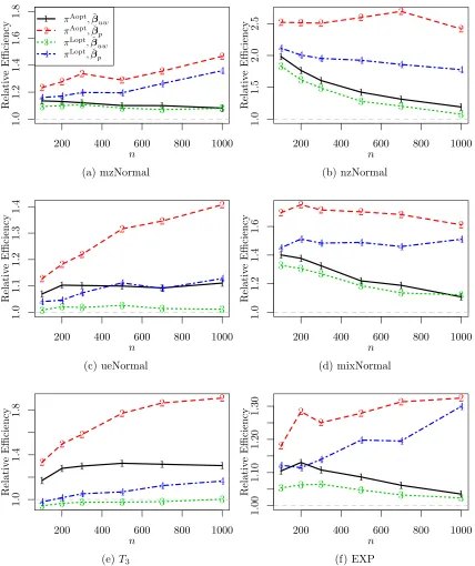
To evaluate the estimation performance of the new estimators compared with the original weighted OSMAC estimator, we define the estimation efficiency of ˇβnew relative to ˇβw as
Relative Efficiency = MSE(ˇβw) MSE(ˇβnew),
where ˇβnew= ˇβuwfor the subsampling with replacement estimator described in Algorithm 1 and ˇβnew = ˇβp for Poisson subsampling estimator described in Algorithm 2. We calculate empirical MSEs from S= 1000 subsamples using
MSE(ˇβ) = 1 S
S
X
s=1
kβˇ(s)−βtk2, (25)
where ˇβ(s) is the estimate from the s-th subsample. We fixed the first step sample size n0= 200 and choose nto be 100, 200, 400, 600, 800, and 1000. This is the same setup used in Wang et al. (2018).
Figure 1 presents the relative efficiency of ˇβuw and ˇβp based on two different choices of πOS
i : π Aopt
i and π
Lopt
i . It is seen that in general ˇβuw and ˇβp are more efficient than ˇ
βw. Among the six cases, the only case that ˇβw can be more efficient is when x has aT3 distribution andπLopt is used, but the difference is not very significant. For all other cases,
ˇ
βuw and ˇβp are more efficient. For example, whenxhas the nzNormal distribution, ˇβp can be 250% as efficient as ˇβw ifπAopt is used. Between ˇβ
uw and ˇβp, ˇβp is more efficient than ˇ
βuw for all cases. We also calculate the empirical unconditional MSE by generating the full data in each repetition of the simulation. The results are similar and thus are omitted.
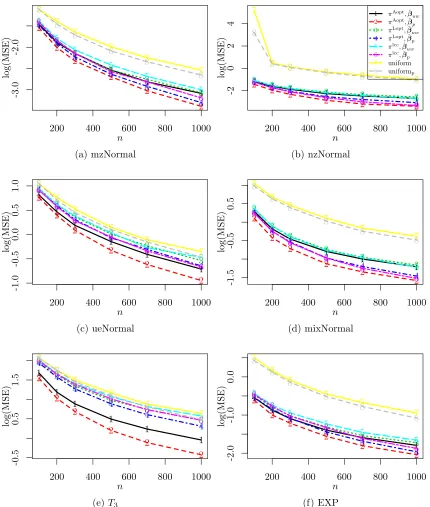
To evaluate the performance of the proposed method with different choices of the sub-sampling probabilities for subsub-sampling with replacement and Poisson subsub-sampling, Figure 2 plots empirical MSEs of usingπAopt,πLopt, πlcc (local case-control), and the uniform sub-sampling probability. In general,πAoptwith Poisson subsampling has the smallest empirical MSEs while uniform subsampling with replacement has the worst estimation efficiency. This agrees with our theoretical results: 1)πAopt minimizes the asymptotic MSE of the parame-ter estimator which corresponds to the empirical MSE defined in (25) for the experiments, while πLopt minimizes the asymptotic MSE of a transformed parameter estimator, and 2) Poisson subsampling has a higher estimation efficiency compared with subsampling with replacement.
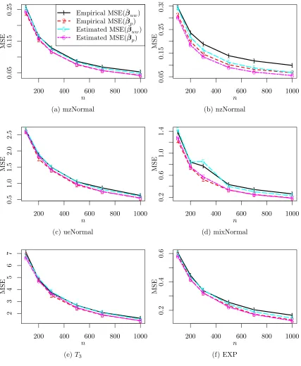
that our purpose here is to evaluate the quality of ˆV(ˇβuw) in (19) and ˆV(ˇβp) in (20), so in this figure we plot the original empirical and estimated MSEs without scaling then using the MSEs of ˇβw. Here, a closer value between the estimated MSE and the empirical MSE indicates a better performance of ˆV(ˇβuw) or ˆV(ˇβp). From Figure 3, the estimated MSEs are very close to the empirical MSEs, except for the case of nzNormal covariate for subsampling with replacement. In this case, the responses are imbalanced with about 95% being 1’s. For this scenario, the variance-covariance estimator for ˇβw proposed in Wang et al. (2018) also has a similar problem of underestimation. For Poisson subsampling, the problem of underestimation from ˆV(ˇβp) is not significant.
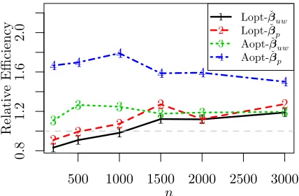
We also apply the more efficient estimation methods to a supersymmetric (SUSY) bench-mark data set (Baldi et al., 2014) available from the Machine Learning Repository (Dua and Karra Taniskidou, 2017). The data set contains a binary response variable indicating whether a process produces new supersymmetric particles or not and 18 covariates that are kinematic features about the process. The full sample size isN = 5,000,000 and the data file is about 2.4 gigabytes. About 54.24% of the responses in the full data are from the background process. We use the more efficient estimation methods with subsample size n to estimate parameters in logistic regression.
Figures 4 gives the relative efficiency of ˇβuw and ˇβp to ˇβw for both πLopti andπAopti . It is seen that whenπAopti are used, ˇβuw and ˇβp always outperform ˇβw. WhenπLopti are used,
ˇ
1 1 1 1 1 1
200 400 600 800 1000
1.0 1.2 1.4 1.6 1.8 n Relativ e Efficiency 2 2 2 2 2 2
3 3 3 3 3 3
4 4 4 4
4 4 1 2 3 4
πAopt,βˇ uw
πAopt,βˇ
p
πLopt,βˇ
uw
πLopt,βˇ
p (a) mzNormal 1 1 1 1 1 1
200 400 600 800 1000
1.0 1.5 2.0 2.5 n Relativ e Efficiency
2 2 2 2
2 2 3 3 3 3 3 3 4
4 4 4
4 4
(b) nzNormal
1 1 1 1 1 1
200 400 600 800 1000
1.0 1.1 1.2 1.3 1.4 n Relativ e Efficiency 2 2 2 2 2 2
3 3 3 3 3 3
4 4 4
4 4 4
(c) ueNormal
1 1
1
1 1
1
200 400 600 800 1000
1.0 1.2 1.4 1.6 n Relativ e Efficiency
2 2 2 2 2
2
3 3 3
3
3 3
4 4 4 4 4 4
(d) mixNormal
1
1 1 1 1 1
200 400 600 800 1000
1.0 1.4 1.8 n Relativ e Efficiency 2 2 2 2 2 2
3 3 3 3 3 3
4 4 4 4
4 4
(e)T3
1 1 1
1
1
1
200 400 600 800 1000
1.00 1.10 1.20 1.30 n Relativ e Efficiency 2 2 2 2 2 2
3 3 3 3
3 3
4 4 4
4 4
4
(f) EXP
1 1 1 1 1 1
200 400 600 800 1000
-3.0 -2.0 n log(MSE) 2 2 2 2 2 2 3 3 3 3 3 3 4 4 4 4 4 4 5 5 5 5 5 5 6 6 6 6 6 6 7 7 7 7 7 7 8 8 8 8 8 8 (a) mzNormal 1 1 1 1 1 1
200 400 600 800 1000
-2 0 2 4 n log(MSE) 2 2 2 2 2 2 3 3 3 3 3 3 4 4 4 4 4 4 5 5 5 5 5 5 6 6 6 6 6 6 7 7 7 7 7 7 8 8 8 8 8 8 1 2 3 4 5 6 7 8
πAopt,βˇ
uw πAopt,βˇ
p πLopt,βˇuw πLopt,βˇp
πlcc,βˇ
uw πlcc,βˇp
uniform uniformp (b) nzNormal 1 1 1 1 1 1
200 400 600 800 1000
-1.0 -0.5 0.0 0.5 1.0 n log(MSE) 2 2 2 2 2 2 3 3 3 3 3 3 4 4 4 4 4 4 5 5 5 5 5 5 6 6 6 6 6 6 7 7 7 7 7 7 8 8 8 8 8 8 (c) ueNormal 1 1 1 1 1 1
200 400 600 800 1000
-1.5 -0.5 0.5 n log(MSE) 2 2 2 2 2 2 3 3 3 3 3 3 4 4 4 4 4 4 5 5 5 5 5 5 6 6 6 6 6 6 7 7 7 7 7 7 8 8 8 8 8 8 (d) mixNormal 1 1 1 1 1 1
200 400 600 800 1000
-0.5 0.5 1.5 n log(MSE) 2 2 2 2 2 2 3 3 3 3 3 3 4 4 4 4 4 4 5 5 5 5 5 5 6 6 6 6 6 6 7 7 7 7 7 7 8 8 8 8 8 8 (e)T3 1 1 1 1 1 1
200 400 600 800 1000
-2.0 -1.0 0.0 n log(MSE) 2 2 2 2 2 2 3 3 3 3 3 3 4 4 4 4 4 4 5 5 5 5 5 5 6 6 6 6 6 6 7 7 7 7 7 7 8 8 8 8 8 8 (f) EXP
1 1 1 1 1 1
200 400 600 800 1000
0.05 0.15 0.25 n MSE 2 2 2 2 2 2 1 2 5 6
Empirical MSE(ˇβuw)
Empirical MSE(ˇβp)
Estimated MSE(ˇβuw)
Estimated MSE(ˇβp) 5 5 5 5 5 5 6 6 6 6 6 6 (a) mzNormal 1 1 1 1 1 1
200 400 600 800 1000
0.05 0.15 0.25 0.35 n MSE 2 2 2 2 2 2 5 5 5 5 5 5 6 6 6 6 6 6 (b) nzNormal 1 1 1 1 1 1
200 400 600 800 1000
0.5 1.0 1.5 2.0 2.5 n MSE 2 2 2 2 2 2 5 5 5 5 5 5 6 6 6 6 6 6 (c) ueNormal 1 1 1 1 1 1
200 400 600 800 1000
0.2 0.6 1.0 1.4 n MSE 2 2 2 2 2 2 5 5 5 5 5 5 6 6 6 6 6 6 (d) mixNormal 1 1 1 1 1 1
200 400 600 800 1000
2 3 4 5 6 7 n MSE 2 2 2 2 2 2 5 5 5 5 5 5 6 6 6 6 6 6 (e)T3 1 1 1 1 1 1
200 400 600 800 1000
0.2 0.4 0.6 n MSE 2 2 2 2 2 2 5 5 5 5 5 5 6 6 6 6 6 6 (f) EXP
1 1
1 1 1
1
500 1000 1500 2000 2500 3000
0.8
1.2
1.6
2.0
n
Relativ
e
Efficiency
2 2 2
2 2
2
3
3 3 3 3 3
4 4 4 4 4
4 1
2
3 4
Lopt-ˇβuw Lopt-ˇβp Aopt-ˇβuw Aopt-ˇβp
Figure 4: Relative efficiency for the SUSY data set with n0 = 200 and different second step subsample sizen. The gray horizontal dashed line is the reference line when relative efficiency is one.
8.2. Computational efficiency
We consider the computational efficiency of the more efficient estimation methods in this section. Note that they have the same order of computational time complexity, so they should have similar computational efficiency as the weighted estimator. For Poisson sub-sampling, there is no need to calculate {πip}N
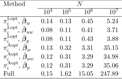
i=1 all at once and random numbers can be generated on the go, so it requires less RAM and may require less CPU times as well. To confirm this, we record the computing time of implementing each of them for the case when x is mzNormal. All methods are implemented in the R programming language (R Core Team, 2017), and computations are carried out on a desktop running Ubuntu Linux 16.04 with an Intel I7 processor and 16GB RAM. Only one logical CPU is used for the calculation. We set the value of dtod= 50, the values ofN to be N = 104,105,106 and 107, and the subsample sizes to ben0= 200 and n= 1000.
Table 1: CPU seconds when the full data are generated and kept in the RAM. Here n0 = 200, n = 1000, and the full data size N varies; the covariates are from a d= 50 dimensional multivariate normal distribution.
Method N
104 105 106 107 πLopti , ˇβw 0.14 0.13 0.45 5.24 πLopti , ˇβuw 0.08 0.11 0.41 3.71 πLopti , ˇβp 0.08 0.11 0.43 3.88 πAopti , ˇβw 0.13 0.32 3.31 35.15 πAopti , ˇβuw 0.12 0.31 3.29 34.98 πAopti , ˇβp 0.12 0.31 3.29 35.06 Full 0.15 1.62 15.05 247.89
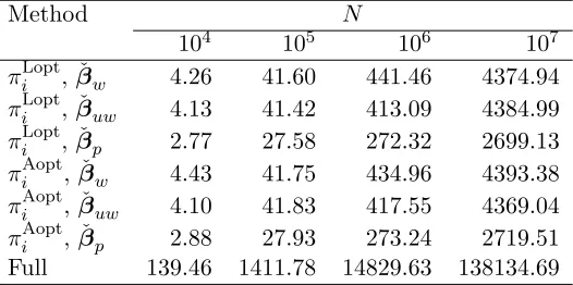
For big data problem, it is common that the full data are larger than the size of the available RAM, and full data can not be loaded into the RAM. For this scenario, one has to load the data into RAM line-by-line or block-by-block. Note that communication between CPU and hard drive is much slower than communication between CPU and RAM. Thus, this will dramatically increase the computing time. To mimic this situation, we store the full data on hard drive and usereadlines()function to process data 1000 rows each time. We also use a smaller computer with 8GB RAM to implement the method. For the case when N = 107, the full data is about 9.1GB which is larger than the available RAM.
Table 2: CPU seconds when the full data are scanned from hard drive. Here n0 = 200, n = 1000, and the full data size N varies; the covariates are from a d = 50 dimensional multivariate normal distribution.
Method N
104 105 106 107 πLopti , ˇβw 4.26 41.60 441.46 4374.94 πLopti , ˇβuw 4.13 41.42 413.09 4384.99 πLopti , ˇβp 2.77 27.58 272.32 2699.13 πAopti , ˇβw 4.43 41.75 434.96 4393.38 πAopti , ˇβuw 4.10 41.83 417.55 4369.04 πAopti , ˇβp 2.88 27.93 273.24 2719.51 Full 139.46 1411.78 14829.63 138134.69
9. Summary
In this paper, we have proposed a new un-weighted estimator for logistic regression based on an OSMAC subsample. We have derived conditional asymptotic distribution of the new estimator which has a smaller variance-covariance matrix compared with the weighted estimator.
We have also investigated the asymptotic properties if Poisson subsampling is used, and showed that the resultant estimator has the same conditional asymptotic distribution if the subsampling ratio converges to zero. However, if the subsampling ratio converges to a positive constant, the estimator based on Poisson subsampling has a smaller variance-covariance matrix.
In addition, we have derive the unconditional asymptotic distribution for the proposed estimator based on Poisson subsampling. Interestingly, if the subsampling ratio converges to zero, the unconditional asymptotic distribution is the same as the conditional asymptotic distribution, indicating that the variation of the full data can be ignored. If the subsampling ratio does not converge to zero, the unconditional asymptotic distribution has a larger variance-covariance matrix. Our results also include the local case-control sampling method. With a stronger moment condition that the third moment of the covariate is finite, we do not require the pilot estimate to be independent of the data.
Furthermore, we have proved consistency and asymptotic normality for the proposed estimators under two types of misspecifications: one is that pilot estimators are inconsistent, and the other is that the logistic regression model is misspecified.
Acknowledgments
Appendix A. Subsampling with replacement from hard drive
If the full data can be loaded into available RAM, subsampling probabilities can be calcu-lated in RAM and subsampling with replacement can be implemented directly. Otherwise, special considerations have to be given in practical implementation. If the full data is larger than available RAM while subsampling probabilities {πOS
i (ˆβ0)}Ni=1 can still be loaded in available RAM, one can calculate {πOS
i (ˆβ0)}Ni=1 by scanning the data from hard drive line-by-line or block-by-block, generate row indexes for a subsample, and then scan the data line-by-line or block-by-block to take the subsample. To be specific, one can draw a subsam-ple, say {idx1, ..., idxn}, from {1, ..., N}, sort the indexes to have {idx(1), ..., idx(n)}, and then use the Algorithm 3 to scan the data line-by-line or block-by-block in order to obtain the subsample.
Algorithm 3 Obtain the subsample with the given indexes by scanning through the full data
Input: data file, subsample indexes{idx(1), ..., idx(n)}. i←1
j ←1
while i≤N andj ≤ndo readline(data file)
if i==idx(j) then
include the i-th data point into the subsample while i==idx(j) do
j ←j+ 1 end while end if i←i+ 1 end while
Clearly, Algorithm 3 takes no more than linear time to run. Here, we assume that a generic function readline() reads a single line (or multiple lines) from the data file and
stop at the beginning of the next line (or next block) in the data file. No calculation is performed on a data line if it is not included in the subsample. Such functionality is provided by most programming languages. For example, Julia (Bezanson et al., 2017) and Python (van Rossum, 1995) has a function readline() that read a file line-by-line; R (R Core Team, 2017) has a functionreadLines()that read one or multiple lines; C (Kernighan and Ritchie, 1988) and C++ (Stroustrup, 1986) has a functiongetline() to read one line at a
time.
Appendix B. Proofs and technical details