Provably Correct Algorithms for Matrix Column Subset Selection with Selectively Sampled Data

Provably Correct Algorithms for Matrix Column Subset

Selection with Selectively Sampled Data

Yining Wang [email protected]

Aarti Singh [email protected]

Machine Learning Department, School of Computer Science Carnegie Mellon University

5000 Forbes Avenue, Pittsburgh, PA 15213, USA

Editor:Sujay Sanghavi

Abstract

We consider the problem of matrix column subset selection, which selects a subset of columns from an input matrix such that the input can be well approximated by the span of the selected columns. Column subset selection has been applied to numerous real-world data applications such as population genetics summarization, electronic circuits testing and recommendation systems. In many applications the complete data matrix is unavailable and one needs to select representative columns by inspecting only a small portion of the input matrix. In this paper we propose the first provably correct column subset selection algorithms for partially observed data matrices. Our proposed algorithms exhibit different merits and limitations in terms of statistical accuracy, computational efficiency, sample complexity and sampling schemes, which provides a nice exploration of the tradeoff between these desired properties for column subset selection. The proposed methods employ the idea of feedback driven sampling and are inspired by several sampling schemes previously introduced for low-rank matrix approximation tasks (Drineas et al., 2008; Frieze et al., 2004; Deshpande and Vempala, 2006; Krishnamurthy and Singh, 2014). Our analysis shows that, under the assumption that the input data matrix has incoherent rows but possibly coherent columns, all algorithms provably converge to the best low-rank approximation of the original data as number of selected columns increases. Furthermore, two of the proposed algorithms enjoy a relative error bound, which is preferred for column subset selection and matrix approximation purposes. We also demonstrate through both theoretical and empirical analysis the power of feedback driven sampling compared to uniform random sampling on input matrices with highly correlated columns.

Keywords: Column subset selection, active learning, leverage scores

1. Introduction

Given a matrix M ∈ Rn1×n2, the column subset selection problem aims to find s exact columns in Mthat capture as much of Mas possible. More specifically, we want to select

s columns of M to form a column sub-matrix C ∈ _Rn1×s _{to minimize the norm of the}

following residue

min

X∈Rs×n2

kM−CXk_ξ=kM−CC†Mk_ξ, (1)

where C† is the Moore-Penrose pseudoinverse of C and ξ = 2 or F denotes the spectral or Frobenius norm. In this paper we mainly focus on the Frobenius norm, as was the

c

case in previous theoretical analysis for sampling based column subset selection algorithms (Drineas et al., 2008; Frieze et al., 2004; Deshpande and Vempala, 2006; Deshpande et al., 2006). To evaluate the performance of column subset selection, one compares the residue norm defined in Eq. (1) with kM−Mkkξ, where Mk is the best rank-kapproximation of

M. Usually the number of selected columnss is larger than or equal to the target rankk. Two forms of error guarantee are common: additive error guarantee in Eq. (2) and relative error guarantee in Eq. (3), with 0< <1 andc >1 (ideallyc= 1 +).

kM−CC†Mk_ξ ≤ kM−Mkkξ+kMkF; (2)

kM−CC†Mk_ξ ≤ ckM−Mkkξ. (3)

In general, relative error bound is much more appreciated becausekMk_ξ is usually large in practice, whilekM−Mkk2is expected to be small when the goal is low-rank approximation.

In addition, when M is an exact low-rank matrix Eq. (3) implies perfect reconstruction, while the error in Eq. (2) remains non-zero. The column subset selection problem can be considered as a form of unsupervised feature selection or prototype selection, which arises frequently in the analysis of large data sets. For example, column subset selection has been applied to various tasks such as summarizing population genetics, testing electronic circuits, recommendation systems, etc. Interested readers should refer to (Boutsidis et al., 2009; Balzano et al., 2010a) for further motivations.

Many methods have been proposed for the column subset selection problem (Chan, 1987; Gu and Eisenstat, 1996; Frieze et al., 2004; Deshpande et al., 2006; Drineas et al., 2008; Boutsidis et al., 2014). An excellent summarization of these methods and their theoretical guarantee is available in Table 1 in (Boutsidis et al., 2009). Most of these methods can be roughly categorized into two classes. One class of algorithms are based on rank-revealing QR (RRQR) decomposition (Chan, 1987; Gu and Eisenstat, 1996) and it has been shown in (Boutsidis et al., 2009) that RRQR is nearly optimal in terms of residue norm under the

s=k setting, that is, exactk columns are selected to reconstruct an input matrix. On the other hand, sampling based methods (Frieze et al., 2004; Deshpande et al., 2006; Drineas et al., 2008) try to select columns by sampling from certain distributions over all columns of an input matrix. Extension of sampling based methods to general low-rank matrix approximation problems is also investigated (Cohen et al., 2015; Bhojanapalli et al., 2015). These algorithms are much faster than RRQR and achieves comparable performance if the sampling distribution is carefully selected and slight over-sampling (i.e., s > k) is allowed (Deshpande et al., 2006; Drineas et al., 2008). In (Boutsidis et al., 2009) sampling based and RRQR based algorithms are unified to arrive at an efficient column subset selection method that uses exactlys=kcolumns and is nearly optimal.

of handling missing data in an elegant way. Below we identify a few key challenges that prevent application of previous theoretical results on column subset selection under the missing data setting:

• Coherent matrix design: most previous results on the completion or recovery of low rank matrices with incomplete data assume the underlying data matrix is incoherent

(Recht, 2011; Candes and Plan, 2010; Keshavan et al., 2010), which intuitively assumes all rows and columns in the data matrix are weakly correlated. 1 On the other hand, previous algorithms on column subset selection and matrix CUR decomposition spent most efforts on dealing with coherent matrices (Deshpande et al., 2006; Drineas et al., 2008; Boutsidis et al., 2009; Boutsidis and Woodruff, 2014). In fact, one can show that under standard incoherence assumptions of matrix completion algorithms a high-quality column subset can be obtained by sampling each column uniformly at random, which trivializes the problem (Xu et al., 2015). Such gap in problem assumptions renders column subset selection on incomplete coherent matrices particularly difficult. In this paper, we explore the possibility of a weaker incoherence assumption that bridges the gap. We present and discuss detailed assumptions considered in this paper in Sec. 1.1.

• Limitation of existing sampling schemes: previous matrix completion methods usually assume the observed data are sampled uniformly at random. However, in (Krishnamurthy and Singh, 2014) it is proved that uniform sampling (in fact any sampling scheme with apriori fixed sampling distribution) is not sufficient to complete a coherent matrix. Though in (Chen et al., 2013) a provably correct sampling scheme was proposed for any matrix based on statistical leverage scores, which is also the key ingredient of many previous column subset selection and matrix CUR decomposition algorithms (Drineas et al., 2008; Boutsidis et al., 2009; Boutsidis and Woodruff, 2014), it is very difficult to approximate the leverage scores of an incomplete coherent matrix. Common perturbation results on singular vector space (e.g., Wedin’s theorem) fail because closeness between two subspaces does not imply closeness in their leverage scores since the latter are defined in an infinity norm manner (see Section 2.1 for details).

• Limitation of zero filling: A straightforward algorithm for missing data column subset selection is to first fill all unobserved entries with zero and then properly scale the observed ones so that the completed matrix is consistent with the underlying data matrix in expectation (Achlioptas and McSherry, 2007; Achlioptas et al., 2013). Column subset selection algorithms designed for fully observed data could be applied afterwards on the zero-filled matrix. However, the zero filling procedure can change the underlying subspace of a matrix drastically (Balzano et al., 2010b) and usually leads to additive error bounds as in Eq. (2). To achieve stronger relative error bounds we need an algorithm that goes beyond the zero filling idea.

In this paper, we propose three column subset selection algorithms based on the idea of active sampling of the input matrix. In our algorithms, observed matrix entries are

chosen sequentially and in a feedback-driven manner. We motivate this sampling setting from both practical and theoretical perspectives. In applications where each entry of a data matrix M represents results from an expensive or time-consuming experiment, it makes sense to carefully select which entry to query (experiment), possibly in a feedback-driven manner, so as to reduce experimental cost. For example, if M has drugs as its columns and targets (proteins) as its rows, it makes sense to cautiously select drug-target pairs for sequential experimental study in order to find important drugs/targets with typical drug-target interactions. From a theoretical perspective, we show in Section 7.1 that no passive sampling scheme is capable of achieving relative-error column subset selection with high probability, even if the column space of M is incoherent. Such results suggest that active/adaptive sampling is to some extent unavoidable, unless both row and column spaces of Mare incoherent.

We also remark that the algorithms we consider make very few measurements of the input matrix, which differs from previous feedback-driven re-sampling methods in the the-oretical computer science literature (e.g., (Wang and Zhang, 2013)) that requires access to the entire input matrix. Active sampling has been shown to outperform all passive schemes in several settings (cf. (Haupt et al., 2011; Kolar et al., 2011)), and furthermore it works for completion of matrices with incoherent rows/columns under which passive learning provably fails (Krishnamurthy and Singh, 2013, 2014). To the best of our knowledge, the algorithms proposed in this paper are the first column subset selection algorithms for coherent ma-trices that enjoy theoretical error guarantee with missing data, whether passive or active. Furthermore, two of our proposed methods achieve relative error bounds.

1.1 Assumptions

Completing/approximating partially observed low-rank matrices using a subset of columns requires certain assumptions on the input data matrix M (Candes and Plan, 2010; Chen et al., 2013; Recht, 2011; Xu et al., 2015). To see this, consider the extreme-case example where the input data matrixMconsists of exactly one non-zero element (i.e.,Mij = 1{i=

i∗, j=j∗}for somei∗∈[n1] andj∗ ∈[n2]). In this case, the relative approximation quality

c=kM−CC†Mk_ξ/kM−M1k_ξ in Eq. (3) would be infinity if columnj∗ is not selected in

C. In addition, it is clearly impossible to correctly identify j∗ using o(n1n2) observations

even with active sampling strategies. Therefore, additional assumptions onMare required to provably approximate a partially observed matrix using column subsets.

In this work we consider the assumption that the top-k column space of the input matrix Mis incoherent (detailed mathematical definition given in Sec. 2.1), while placing no incoherence or spikiness assumptions on the actualcolumns, rows or the row space ofM. In addition to the necessity of incoherence assumptions for incomplete matrix approximation problems discussed above, we further motivate the “one-sided” incoherence assumption from two perspectives:

subset selection algorithms for fully-observed matrices also need to be majorly revised to accommodate missing matrix components.

- Compared to existing work on approximating low-rank incomplete matrices, our as-sumptions (one-sided incoherence) are arguably weaker. Xu et al. (2015) analyzed matrix CUR approximation of partially observed matrices, but assumed that both column and row spaces are incoherent; Krishnamurthy and Singh (2014) derived an adaptive sampling procedure to complete a low-rank matrix with only one-sided in-coherence assumptions, but only achieved additive error bounds for noisy low-rank matrices.

- Finally, the one-sided incoherence assumption is reasonable in a number of practical scenarios. For example, in the application of drug-target interaction prediction, the one-sided incoherence assumption allows for highly specialized or diverse drugs while assuming some predictability between target protein responses.

1.2 Our contributions

The main contribution of this paper is three provably correct algorithms for column subset selection, which are inspired by existing work on column subset selection for fully-observed matrices, but only inspect a small portion of the input matrix. The sampling schemes for the proposed algorithms and their main merits and drawbacks are summarized below:

1. Norm sampling: The algorithm is simple and works for any input matrix with incoherent column subspace. However, it only achieves an additive error bound as in Eq. (2). It is also inferior than the other two proposed methods in terms of residue error on both synthetic and real-world data sets.

2. Iterative norm sampling: The iterative norm sampling algorithm enjoys relative error guarantees as in Eq. (3) at the expense of being much more complicated and computationally expensive. In addition, its correctness is only proved for low-rank matrices with incoherent column space corrupted with i.i.d. Gaussian noise.

3. Approximate leverage score sampling: The algorithm enjoys relative error guar-antee for general (high-rank) input matrices with incoherent column space. However, it requires more over-sampling and its error bound is worse than the one for itera-tive norm sampling on noisy low-rank matrices. Moreover, to actually reconstruct the data matrix2 the approximate leverage score sampling scheme requires sampling a subset of both entire rows and columns, while both norm based algorithms only require sampling of some entire columns.

In summary, our proposed algorithms offer a rich, provably correct toolset for column subset selection with missing data. Furthermore, a comprehensive understanding of the de-sign tradeoffs among statistical accuracy, computational efficiency, sample complexity, and sampling scheme, etc. is achieved by analyzing different aspects of the proposed methods. Our analysis could provide further insights into other matrix completion/approximation tasks on partially observed data.

We also perform comprehensive experimental study of column subset selection with missing data using the proposed algorithms as well as modifications of heuristic algorithms proposed recently (Balzano et al., 2010a; Bien et al., 2010) on synthetic matrices and two real-world applications: tagging Single Nucleotide Polymorphisms (tSNP) selection and column based image compression. Our empirical study verifies most of our theoretical re-sults and reveals a few interesting observations that are previously unknown. For instance, though leverage score sampling is widely considered as the state-of-the-art for matrix CUR approximation and column subset selection, our experimental results show that under cer-tain low-noise regimes (meaning that the input matrix is very close to low rank) iterative norm sampling is more preferred and achieves smaller error. These observations open new questions and suggest the need for new analysis in related fields, even for the fully observed case.

1.3 Notations

For any matrixMwe useM(i) to denote thei-th column ofM. Similarly,M(i) denotes the

i-th row ofM. All norms k · kare `2 norms or the matrix spectral norm unless otherwise

specified.

We assume the input matrix is of size n1×n2, n = max(n1, n2). We further assume

that n1 ≤n2. We use xi =M(i) ∈Rn1 to denote the i-th column of M. Furthermore, for any column vector xi ∈Rn1 and index subset Ω⊆[n1], define the subsampled vector xi,Ω

and the scaled subsampled vector RΩ(xi) as

xi,Ω =1Ω◦xi, RΩ(xi) =

n1

|Ω|1Ω◦xi, (4)

where1Ω ∈ {0,1}n1 _{is the indicator vector of Ω and◦ is the Hadamard product (entrywise}

product). We also generalize the definition in Eq. (4) to matrices by applying the same operator on each column.

We use kM−CC†Mkξ to denote the selection error and kM−CXkξ to denote the

reconstruction error. The difference between the two types of error is that for selection error an algorithm is only required to output indices of the selected columns while for reconstruction error an algorithm needs to output both the selected columns C and the coefficient matrix X so that CX is close to M. We remark that the reconstruction error always upper bounds the selection error due to Eq. (1). On the other hand, there is no simple procedure to computeC†M whenM is not fully observed.

1.4 Outline of the paper

2. Preliminaries

This section provides necessary background knowledge for the analysis in this paper. We first review the concept of coherence, which plays an important row in sampling based matrix algorithms. We then summarize three matrix sampling schemes proposed in previous literature.

2.1 Subspace and vector incoherence

Incoherence plays a crucial role in various matrix completion and approximation tasks (Recht, 2011; Krishnamurthy and Singh, 2014; Candes and Plan, 2010; Keshavan et al., 2010). For any matrix M ∈ _Rn1×n2 _{of rank k, singular value decomposition yields M =}

UΣV>, where U ∈ _Rn1×k _{and V ∈}

Rn2×k have orthonormal columns. Let U = span(U) and V = span(V) be the column and row space of M. The column space coherence is defined as

µ(U) := n1

k

n1

max i=1 kU

>_e ik22 =

n1

k

n1

max i=1 kU(i)k

2

2. (5)

Note thatµ(U) is always between 1 andn1/k. Similarly, therow space coherence is defined

as

µ(V) := n2

k

n2

max i=1 kV

>_e ik22 =

n2

k

n2

max i=1 kV(i)k

2

2. (6)

In this paper we also make use of incoherence level of vectors, which previously appeared in (Balzano et al., 2010b; Krishnamurthy and Singh, 2013, 2014). For a column vector

x∈_Rn1_{, its incoherence is defined as}

µ(x) := n1kxk

2

∞ kxk2

2

. (7)

It is an easy observation that if x lies in the subspace U then µ(x) ≤ kµ(U). In this paper we adopt incoherence assumptions on the column spaceU, which subsequently yields incoherent row vectors xi. No incoherence assumption on the row space V or row vectors

M_(i) is made.

2.2 Matrix sampling schemes

Norm sampling: Norm sampling for column subset selection was proposed in (Frieze et al., 2004) and has found applications in a number of matrix computation tasks, e.g., approx-imate matrix multiplication (Drineas et al., 2006a) and low-rank or compressed matrix approximation (Drineas et al., 2006c,b). The idea is to sample each column with proba-bility proportional to its squared `2 norm, i.e., Pr[i∈ C]∝ kM(i)k22 fori∈ {1,2,· · ·, n2}.

These types of algorithms usually come with an additive error bound on their approximation performance.

Volume sampling: For volume sampling (Deshpande et al., 2006), a subset of columnsC

is picked with probability proportional to the volume of the simplex spanned by columns in

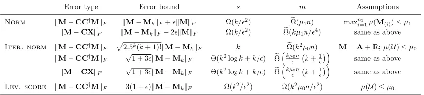
Table 1: Summary of theoretical guarantees of proposed algorithms. s denotes the num-ber of selected columns and m denotes the expected number of observed matrix entries. Dependency on failure probabilityδ and other poly-logarithmic dependency is omitted. U represents the column space of A.

Error type Error bound s m Assumptions

Norm kM−CC†_Mk

F kM−MkkF+kMkF Ω(k/2) Ω(e µ1n) max

n2

i=1µ(M(i))≤µ1 kM−CXkF kM−MkkF+ 2kMkF Ω(k/2) Ω(e kµ1n/4) same as above

Iter. norm kM−CC†MkF p

2.5k_{(k+ 1)!kM−M}

kkF k Ω(e k2µ0n) M=A+R;µ(U)≤µ0

kM−CC†MkF

√

1 + 3kM−MkkF Θ(k2logk+k/) Ωe

_kµ

0n

k+

1

same as above

kM−CXkF

√

1 + 3kM−MkkF Θ(k2logk+k/) Ωe

kµ0n

k+

1

same as above

Lev. score kM−CC†_Mk

F 3(1 +)kM−MkkF Ω(k2/2) Ω(k2µ0n/2) µ(U)≤µ0

MCMC sampling procedure (Anari et al., 2016). Under the partially observed setting, both approaches are difficult to apply. For the characteristic polynomials approach, one has to estimate the characteristic polynomial and essentially the least singular value of the target matrix Mup to relative error bounds. This is not possible unless the matrix is very well-conditioned, which violates the setting thatMis approximately low-rank. For the MCMC sampling procedure, it was shown in (Anari et al., 2016) thatO(kn2) iterations are needed

for the sampling Markov chain to mix. As each sampling iteration requires observing one entire column, performingO(kn2) iterations essentially requires observingO(kn2) columns,

i.e., the entire matrix M. On the other hand, an iterative norm sampling procedure is known to perform approximate volume sampling and therefore enjoys multiplicative ap-proximation bounds for column subset selection (Deshpande and Vempala, 2006). In this paper we generalize the iterative norm sampling scheme to the partially observed setting and demonstrate similar multiplicative approximation error guarantees.

Leverage score sampling: The leverage score sampling scheme was introduced in (Drineas et al., 2008) to get relative error bounds for CUR matrix approximation and has later been applied to coherent matrix completion (Chen et al., 2013). For each row i ∈ {1,· · · , n1}

and column j ∈ {1,· · · , n2} define µi := n_k1kU>eik22 and νj := n_k2kV>ejk22 to be their unnormalized leverage scores, where U ∈ _Rn1×k _{and V ∈}

Rn2×k are the top-k left and right singular vectors of an input matrixM. It was shown in (Drineas et al., 2008) that if rows and columns are sampled with probability proportional to their leverage scores then a relative error guarantee is possible for matrix CUR approximation and column subset selection.

3. Column subset selection via active sampling

Algorithm 1 Active norm sampling for column subset selection with missing data

1: Input: size of column subset s, expected number of samples per column m1 andm2.

2: Norm estimation: For each column i, sample each index in Ω1,i ⊆ [n1] i.i.d. from

Bernoulli(m1/n1). observe xi,Ω1,i and compute ˆci =

n1

m1kxi,Ω1,ik

2

2. Define ˆf = P

icˆi.

3: Column subset selection: SetC=0∈_Rn1×s_.

• Fort∈[s]: sample it∈[n2] such that Pr[it=j] = ˆcj/fˆ. ObserveM(it) in full and setC(t) _=M(it)_.

4: Matrix approximation: SetMc =0∈Rn1×n2.

• For each columnxi, sample each index in Ω2,i⊆[n1] i.i.d. from Bernoulli(m2,i/n1),

wherem2,i=m2n2ˆci/fˆ; observexi,Ω2,i.

• Update: Mc =Mc+ (R_Ω2,i(xi))e>_i .

5: Output: selected columnsC and coefficient matrixX=C†Mc.

and more sampled columns. Table 1 summarizes the main theoretical guarantees for the proposed algorithms.

3.1 `2 norm sampling

We first present an active norm sampling algorithm (Algorithm 1) for column subset selec-tion under the missing data setting. The algorithm is inspired by the norm sampling work for column subset selection by Frieze et al. (Frieze et al., 2004) and the low-rank matrix approximation work by Krishnamurthy and Singh (Krishnamurthy and Singh, 2014).

The first step of Algorithm 1 is to estimate the `2 norm for each column by uniform

subsampling. Afterwards, s columns of M are selected independently with probability proportional to their`2 norms. Finally, the algorithm constructs a sparse approximation of

the input matrix by sampling each matrix entry with probability proportional to the square of the corresponding column’s norm and then a CXapproximation is obtained.

When the input matrix M has incoherent columns, the selection error as well as CX

reconstruction error can be bounded as in Theorem 1.

Theorem 1 Suppose maxn2

i=1µ(xi) ≤ µ1 for some positive constant µ1. Let C and X be the output of Algorithm 1. Denote Mk as the best rank-k approximation of M. Fix

δ=δ1+δ2+δ3>0. With probability at least 1−δ, we have

kM−CC†MkF ≤ kM−MkkF +kMkF (8)

provided thats= Ω(k−2_/δ

2),m1 = Ω(µ1log(n/δ1)). Furthermore, ifm2 = Ω(µ1slog2(n/δ3)/(δ22)) then with probability ≥1−δ we have the following bound on reconstruction error:

Algorithm 2Active iterative norm sampling for column subset selection for data corrupted by Gaussian noise

1: Input: target rankk <min(n1, n2), error tolerance parameter,δand expected number

of samples per column m.

2: Entrywise sampling: For each columni, sample each index in an index set Ωi ⊆[n1]

i.i.d. from Bernoulli(m/n1). Observexi,Ωi.

3: Approximate volume sampling: SetC =U =∅. LetU be an orthonormal basis of U.

4: fort= 1,2,· · ·, k do

5: For i∈ {1,· · · , n2}, compute ˆci(t)= nm1kxi,Ωi−UΩi(U >

ΩiUΩi)−1U>Ωixi,Ωik22.

6: Set ˆf(t)=Pn2

i=1ˆc (t)

i .

7: Select a column it at random, with probability Pr[it=j] = ˆp

(t)

j = ˆc

(t)

j /fˆ(t).

8: Observe M(it) in full and update: C ←C∪ {it},U ←span(U,{M(it)}).

9: end for

10: Active norm sampling: set T = (k+ 1) log(k+ 1) ands1 =s2 =· · · =sT−1 = 5k,

sT = 10k/δ;S =∅,S =∅. SupposeU is an orthonormal basis of span(U,S).

11: fort= 1,2,· · ·, T do

12: For i∈ {1,· · · , n2}, compute ˆci(t)= nm1kxi,Ωi−UΩi(U >

ΩiUΩi)−1U>Ωixi,Ωik22.

13: Set ˆf(t)=Pn2

i=1ˆc (t)

i .

14: SelectstcolumnsSt= (i1,· · · , ist) independently at random, with probability Pr[j∈

St] = ˆq(jt)= ˆc

(t)

j /fˆ(t).

15: Observe M(St) in full and update: S←S∪St,S ←span(S,{M(St)}).

16: end for

17: Matrix approximation: Mc= Pn2

i=1U(U

>

ΩiUΩi)

−1_UΩix

i,Ωie>i , whereU∈Rn1×(s+k) is an orthonormal basis of span(U₀,U₁).

18: Output: selected column subsets C = (M(C(1))_{,· · · ,M}(C(k))_{) ∈}

Rn1×k, S = (M(C)_,M(S1)_{,· · ·,M}(ST)_)∈Rn1×s _{where s=k+s}

1+· · ·+sT and X=SS†Mc.

As a remark, Theorem 1 shows that one can achieveadditive reconstruction error using Algorithm 1 with expected sample complexity (omitting dependency onδ)

Ω

µ1n2log(n) +

kn1

2 +

kµ1n2log2(n)

4

= Ω(kµ1−4nlog2n).

3.2 Iterative norm sampling

In this section we present Algorithm 2, another active sampling algorithm based on the idea of iterative norm sampling and approximate volume sampling introduced in (Deshpande and Vempala, 2006). Though Algorithm 2 is more complicated than Algorithm 1, it achieves a relative error bound on inputs that are noisy perturbation of some underlying low-rank matrix.

Algorithm 2 employs the idea of iterative norm sampling. That is, after selecting l

spanned by currently selected columns. It can be shown that iterative norm sampling serves as an approximation ofvolume sampling, a sampling scheme that is known to have relative error guarantees (Deshpande et al., 2006; Deshpande and Vempala, 2006).

Theorem 2 shows that when the input matrix M is the sum of an exact low rank matrix A and a stochastic noise matrix R, then by selecting exact k columns from M

using iterative norm sampling one can upper bound the selection errorkM−CC†Mk_F by the best rank-k approximation error kM−MkkF within a multiplicative factor that does not depend on the matrix size n. Such relative error guarantee is much stronger than the additive error bound provided in Theorem 1 as when M is exactly low rank the error is eliminated with high probability. In fact, when the input matrix M is exactly low rank the first phase of the proposed algorithm (Line 1 to Line 9 in Algorithm 2) resembles the adaptive sampling algorithm proposed in (Krishnamurthy and Singh, 2013, 2014) for matrix and tensor completion in the sense that at each iteration all columns falling exactly onto the span of already selected columns will have zero norm after projection and hence will never be sampled again. However, we are unable to generalize our algorithm to general full-rank inputs because it is difficult to bound the incoherence level of projected columns (and hence the projection accuracy itself later on) without a stochastic noise model. We present a new algorithm with slightly worse error bounds in Section 3.3 which can handle general high-rank inputs.

Though Eq. (10) is a relative error bound, the multiplicative factor scales exponentially with the intrinsic rank k, which is not completely satisfactory. As a remedy, we show that by slightly over-sampling the columns (Θ(k2logk+k/δ) instead ofkcolumns) the selection error as well as theCXreconstruction error could be upper bounded bykM−MkkF within only a (1 + 3) factor, which implies that the error bounds are nearly optimal when the number of selected columns sis sufficiently large, for example, s= Ω(k2logk+k/δ).

Theorem 2 Fix δ > 0. Suppose M =A+R, where A is a rank-k deterministic matrix with incoherent column space (i.e., µ(U(A)) ≤ µ0) and R is a random matrix with i.i.d. zero-mean Gaussian distributed entries. Suppose k=O(n1/log(n2/δ)). Let C,S and X be the output of Algorithm 2. Then the following holds:

1. If m= Ω(k2µ0log2(n/δ))then with probability ≥1−δ

kM−CC†Mk2_F ≤ 2.5

k_{(k+ 1)!}

δ kRk

2

F. (10)

The column subset size iskand the corresponding sample complexity isΩ(k2µ0nlog2(n/δ)). 2. If m= Ω(−1sµ0log2(n/δ))withs= Θ(k2logk+k/δ), then with probability ≥1−δ

kM−SS†Mk2_F ≤ kM−SXk2_F ≤(1 + 3)kRk2_F. (11)

The column subset size is Θ(k2logk+k/δ) and the sample complexity is (omitting dependence on δ)

Ω

k2µ0nlogklog2(n)

+

kµ0nlog2(n)

2

Algorithm 3 Approximate leverage score sampling for column subset selection on general input matrices

1: Input: target rankk, size of column subset s, expected number of row samples m.

2: Leverage score estimation: SetS=∅.

• For each row i, with probability m/n1 observe the row M(i) in full and update

S ←span(S,{M(i)}).

• Compute the first k right singular vectors of S (denoted by Sk ∈ Rn2×k) and estimate the unnormalized row space leverage scores as ˜lj = kSk>ejk22,

j∈ {1,2,· · ·, n1}.

3: Column subset selection: SetC=∅.

• For t∈ {1,2,· · ·, s} select a column it ∈ [n2] with probability P r[it =j] = ˆpj = ˜

lj/k; updateC ←C∪ {it}.

4: Output: the selected column indices C ⊆ {1,2,· · · , n2} and actual columns C =

(M(C(1)),· · · ,M(C(s))).

3.3 Approximate leverage score sampling

The third sampling-based column subset selection algorithm for partially observed matrices is presented in Algorithm 3. The proposed algorithm was based on the leverage score sampling scheme for matrix CUR approximation introduced in (Drineas et al., 2008). To compute the sampling distribution (i.e., leverage scores) from partially observed data, the algorithm subsamples a small number of rows from the input matrix and uses leverage scores of the row space of the subsampled matrix to form the sampling distribution. Note that we do not attempt to approximate leverage scores of the original input matrix directly; instead, we compute leverage scores of another matrix that is a good approximation of the original data. Such technique was also explored in (Drineas et al., 2012) to approximate statistical leverages in a fully observed setting. Afterwards, column sampling distribution is constructed using the estimated leverage scores and a subset of columns are selected according to the constructed sampling distribution.

We bound the selection errorkM−CC†MkF of the approximate leverage score sampling algorithm in Theorem 3. Note that unlike Theorem 1 and 2, only selection error bound is provided since for deterministic full-rank input matrices it is challenging to approximately compute the projection of M onto span(C) because the projected vector may no longer be incoherent (this is in fact the reason why Theorem 2 holds only for low-rank matrices perturbed by Gaussian noise, and we believe similar conclusion should also hold for Algo-rithm 3 is the stronger assumption of Gaussian noise perturbation is made). It remains an open problem to approximately computeC†MgivenCwith provable guarantee for general matrix M without observing it in full. Eq. (3) shows that Algorithm 3 enjoys a relative error bound on the selection error. In fact, when the input matrix M is exactly low rank then Algorithm 3 is akin to the two-step matrix completion method proposed in (Chen et al., 2013) for column incoherent inputs.

approximate leverage score sampling algorithm compared to the iterative norm sampling method. First, Algorithm 3 always needs to over-sample columns (at the level of Θ(k2/2), which is even more than Algorithm 2 for a (1 +) reconstruction error bound); in contrast, the iterative norm sampling algorithm only requires exactk selected columns to guarantee a relative error bound. In addition, Eq. (12) shows that the selection error bound is suboptimal even ifsis sufficiently large because of the (3 + 3) multiplicative term.

Theorem 3 SupposeMis an input matrix with incoherent top-kcolumn space (i.e.,µ(U_k(M))≤

µ0) and C is the column indices output by Algorithm 3. If m = Ω(−2µ0k2log(1/δ)) and

s= Ω(−2k2log(1/δ))then with probability ≥1−δ the following holds:

kM−CC†MkF ≤3(1 +)kM−MkkF, (12)

where C = [M(C(1)),· · · ,M(C(s))] ∈ _Rn1×s _{are the selected columns and M}

k is the best

rank-k approximation of M.

4. Proofs

In this section we provide proof sketches of the main results (Theorem 1, 2 and 3). Some technical lemmas and complete proof details are deferred to Appendix A and B.

4.1 Proof sketch of Theorem 1

The proof of Theorem 1 can be divided into two steps. First, in Lemma 1 we show that (approximate) column sampling yields an additive error bound for column subset selection. Its proof is very similar to the one presented in (Frieze et al., 2004) and we defer it to Appendix A. Second, we cite a lemma from (Krishnamurthy and Singh, 2014) to show that with high probability the first pass in Algorithm 1 gives accurate estimates of column norms of the input matrix M.

Lemma 1 Provided that (1−α)kxik22 ≤ ˆci ≤ (1 + α)kxik22 for i = 1,2,· · ·, n2, with probability ≥1−δ we have

kM− PC(M)kF ≤ kM−MkkF +

s

(1 +α)k

(1−α)δskMkF, (13)

where Mk is the best rank-kapproximation of M.

Lemma 2 ((Krishnamurthy and Singh, 2014), Lemma 10) Fix α, δ ∈ (0,1). As-sume µ(xi)≤µ0 holds for i= 1,2,· · ·, n2. For some fixedi∈ {1,· · · , n2} with probability

≥1−2δ we have

(1−α)kxik22 ≤cˆi ≤(1 +α)kxik22 (14) withα=

q 2µ0

m1 log(1/δ)+

2µ0

3m1 log(1/δ). Furthermore, ifm1= Ω(µ0log(n2/δ))with carefully

Combining Lemma 1 and Lemma 2 and settings= Ω(k−2/δ) for some target accuracy thresholdwe have that with probability 1−3δ the selection error bound Eq. (8) holds.

In order to bound the reconstruction error kM−CXk2

F, we cite another lemma from (Krishnamurthy and Singh, 2014) that analyzes the performance of the second pass of Algorithm 1. At a higher level, Lemma 3 is a consequence of matrix Bernstein inequality (Tropp, 2012) which asserts that thespectral norm of a matrix can be preserved by a sum of properly scaled randomly sampled sub-matrices.

Lemma 3 ((Krishnamurthy and Singh, 2014), Lemma 9) Provided that(1−α)kxik22≤

ˆ

ci ≤(1 +α)kxik22 for i= 1,2,· · · , n2, with probability ≥1−δ we have

kM−cMk₂≤ kMk_F r

1 +α

1−α

4 3

r

n1µ0

m2n2

log

n1+n2

δ

+

s

4

m2

max

n1

n2

, µ0

log

n1+n2

δ

!

.

(15)

The complete proof of Theorem 1 is deferred to Appendix A.

4.2 Proof sketch of Theorem 2

In this section we give proof sketch of Eq. (10) and Eq. (11) separately.

4.2.1 Proof sketch of kM−CC†MkF error bound

We take three steps to prove the kM−CC†Mk_F error bound in Theorem 2. At the first step, we show that when the input matrix has a low rank plus noise structure then with high probability for all small subsets of columns the spanned subspace has incoherent column space (assuming the low-rank matrix has incoherent column space) and furthermore, the projection of the other columns onto the orthogonal complement of the spanned subspace are incoherent, too. Given the incoherence condition we can easily prove a norm estimation result similar to Lemma 2, which is the second step. Finally, we note that the approxi-mate iterative norm sampling procedure is an approximation ofvolume sampling, a column sampling scheme that is known to yield a relative error bound.

STEP 1: We first prove that when the input matrixMis a noisy low-rank matrix with incoherent column space, with high probability a fixed column subset also has incoherent column space. This is intuitive because the Gaussian perturbation matrix is highly inco-herent with overwhelming probability. A more rigorous statement is shown in Lemma 4.

Lemma 4 Suppose Ahas incoherent column space, i.e.,µ(U(A))≤µ0. FixC⊆[n2]to be any subset of column indices that hasselements andδ >0. LetC= [M(C(1)),· · ·,M(C(s))]∈ Rn1×s be the compressed matrix and U(C) = span(C) denote the subspace spanned by the

selected columns. Suppose max(s, k) ≤ n1/4−k and log(4n2/δ) ≤ n1/64. Then with probability ≥1−δ over the random drawn of R we have

µ(U(C)) = n1

s 1≤maxi≤n1

kPU(C)eik22=O

kµ0+s+

p

slog(n1/δ) + log(n1/δ)

s

!

furthermore, with probability ≥1−δ the following holds:

µ(P_U(C)⊥(M(i))) =O(kµ₀+ log(n₁n₂/δ)), ∀i /∈C. (17)

At a higher level, Lemma 4 is a consequence of the Gaussian white noise being highly incoherent, and the fact that the randomness imposed on each column of the input matrix is independent. The complete proof can be found in Appendix B.

Given Lemma 4, Corollary 1 holds by taking a uniform bound over all Ps

j=1

n2

j

=

O(s(n2)s) column subsets that contain no more thanselements. The 2slog(4n2/δ)≤n1/64

condition is only used to ensure that the desired failure probability δ is not exponentially small. Typically, in practice the intrinsic dimensionkand/or the target column subset size

sis much smaller than the ambient dimensionn1.

Corollary 1 Fix δ > 0 and s ≥ k. Suppose s ≤ n1/8 and 2slog(4n2/δ) ≤ n1/64. With probability≥1−δ the following holds: for any subset C⊆[n2]with at mostselements, the spanned subspace U(C) satisfies

µ(U(C))≤O((k+s)|C|−1µ0log(n/δ)); (18)

furthermore,

µ(P_U(C)⊥(M(i))) =O((k+s)µ₀log(n/δ)), ∀i /∈C. (19)

STEP 2: In this step, we prove that the norm estimation scheme in Algorithm 2 works when the incoherence conditions in Eq. (18) and (19) are satisfied. More specifically, we have the following lemma bounding the norm estimation error:

Lemma 5 Fix i ∈ {1,· · ·, n2}, t ∈ {1,· · · , k} and δ, δ0 > 0. Suppose Eq. (18) and (19) hold with probability≥1−δ. LetSt be the subspace spanned by selected columns at thet-th

round and letcˆ(_it) denote the estimated squared norm of theith column. If m satisfies

m= Ω(kµ0log(n/δ) log(k/δ0)), (20)

then with probability ≥1−δ−4δ0 we have

1

2k[Et](i)k

2 2≤ˆc

(t)

i ≤

5

4k[Et](i)k

2

2. (21)

Here Et=PS⊥

t (M) denotes the projected matrix at the t-th round.

Lemma 5 is similar with previous results on subspace detection (Balzano et al., 2010b) and matrix approximation (Krishnamurthy and Singh, 2014). The intuition behind Lemma 5 is that one can accurately estimate the`2 norm of a vector by uniform subsampling entries of

the vector, provided that the vector itself is incoherent. The proof of Lemma 5 is deferred to Appendix B.

Similar to the first step, by taking a union bound over all possible subsets of picked columns and n2 −k unpicked columns we can prove a stronger version of Lemma 5, as

Corollary 2 Fix δ, δ0>0. Suppose Eq. (18) and (19) hold with probability ≥1−δ. If

m≥Ω(k2µ0log(n/δ) log(n/δ0)) (22)

then with probability≥1−δ−4δ0 the following property holds for any selected column subset by Algorithm 2:

2 5

k[Et](i)k22

kEtk2_F

≤pˆ(_it)≤ 5 2

k[Et](i)k22

kEtk2_F

,∀i∈[n2], t∈[k], (23)

where pˆ(_it)= ˆc_i(t)/fˆ(t) is the sampling probability of theith column at roundt. STEP 3: To begin with, we definevolume sampling distributions:

Definition 1 (volume sampling, (Deshpande et al., 2006)) A distributionpover col-umn subsets of sizek is a volume sampling distribution if

p(C) = vol(∆(C))

2 P

T:|T|=kvol(∆(T))2

, ∀|C|=k. (24)

Volume sampling has been shown to achieve a relative error bound for column subset se-lection, which is made precise by Theorem 4 cited from (Deshpande and Vempala, 2006; Deshpande et al., 2006).

Theorem 4 ((Deshpande and Vempala, 2006), Theorem 4) Fix a matrixMand let Mk denote the best rank-k approximation of M. If the sampling distributionp is a volume

sampling distribution defined in Eq. (24) then

EC

kM− PV(C)(M)k2F

≤(k+ 1)kM−Mkk2F; (25)

furthermore, applying Markov’s inequality one can show that with probability ≥1−δ

kM− P_V(C)(M)k2_F ≤ k+ 1

δ kM−Mkk

2

F. (26)

In general, exact volume sampling is difficult to employ under partial observation set-tings, as we explained in Sec. 2.2. However, in (Deshpande and Vempala, 2006) it was shown that iterative norm sampling serves as an approximate of volume sampling and achieves a relative error bound as well. In Lemma 6 we present an extension of this result. Namely,

approximate iterative column norm sampling is an approximate of volume sampling, too. Its proof is very similar to the one presented in (Deshpande and Vempala, 2006) and we defer it to Appendix B.

Lemma 6 Let p be the volume sampling distribution defined in Eq. (24). Suppose the sampling distribution of a k-round sampling strategy pˆsatisfies Eq. (23). Then we have

ˆ

We can now prove the error bound for selection error kM−CC†Mk_F of Algorithm 2 by combining Corollary 1, 2, Lemma 6 and Theorem 4, with failure probability δ, δ0

set at O(1/k) to facilitate a union bound argument across all iterations. In particular, Corollary 1 and 2 guarantees that Algorithm 2 estimates column norms accurately with high probability; then one can apply Lemma 6 to show that the sampling distribution employed in the algorithm is actually an approximate volume sampling distribution, which is known to achieve relative error bounds (by Theorem 4).

4.2.2 Proof sketch of kM−SXkF error bound

We first present a theorem, which is a generalization of Theorem 2.1 in (Deshpande et al., 2006).

Theorem 5 ((Deshpande et al., 2006), Theorem 2.1) Suppose M ∈ _Rn1×n2 _{is the}

input matrix and U ⊆ Rn1 _{is an arbitrary vector space. Let S ∈ R}n1×s _{be a random}

sample of scolumns in M from a distribution q such that

(1−α)kE(i)k2 2

(1 +α)kEk2

F

≤qi ≤

(1 +α)kE(i)k2 2

(1−α)kEk2

F

, ∀i∈ {1,2,· · · , n2}, (28) where E=P_U⊥(M) is the projection of M onto the orthogonal complement of U. Then

ES

kM− P_span(U,S),k(M)k2F

≤ kM−Mkk2F +

(1 +α)k

(1−α)skEk

2

F, (29)

where Mk denotes the best rank-k approximation of M.

Intuitively speaking, Theorem 5 states that relative estimation of residues P_U⊥(M) would yield relative estimation of the data matrixM itself.

In the remainder of the proof we assumes= Ω(k2log(k)+k/δ) is the number of columns selected in S in Algorithm 2. Corollary 1 asserts that with high probability µ(U(S)) =

O(s|C|−1_µ

0log(n/δ)) andµ(PU(S)⊥(M(i))) =O(sµ₀log(n/δ)) for any subsetSwith|S| ≤s. Subsequently, we can apply Lemma 5 and a union bound overn2 columns andT rounds to

obtain the following proposition:

Proposition 1 Fix δ, δ0 > 0. If m = Ω(sµ0log(n/δ) log(nT /δ0)) then with probability

≥1−δ−δ0

2kE(_ti)k2 2

5kEtk2_F

≤qˆ_i(t)≤ 5kE

(i)

t k22

2kEtk2_F

, ∀i∈ {1,2,· · · , n2}, t∈ {1,2,· · · , T}. (30) HereEt=M−Pspan(U ∪S1∪···∪St−1)(M)is the residue at roundtof the active norm sampling

procedure.

Note that we do not need to take a union bound over all n2

s

column subsets because this time we do not require the sampling distribution of Algorithm 2 to be close uniformly to the true active norm sampling procedure.

Lemma 7 Fix δ, δ0 >0. If m= Ω(sµ0log2(n/δ)) and s1 =· · ·=sT−1 = 5k, sT = 10k/δ0

then with probability ≥1−2δ−δ00

kM− PU ∪S1∪···∪ST(M)k 2

F ≤(1 +/2)kM−Mkk2F +

/2

2T kM− PU(M)k

2

F. (31)

Applying Theorem 4, Lemma 6 and note that 2(k+1) log(k+1) = (k+ 1)(k+1) ≥(k+ 1)!, we immediately have Corollary 3.

Corollary 3 Fix δ > 0. Suppose T = (k+ 1) log(k+ 1) and m, s1,· · · , sT be set as in

Lemma 7. Then with probability ≥1−4δ one has

kM−SS†Mk2_F =kM− PU ∪S1∪···∪ST(M)k 2

F ≤(1 +)kM−MkkF2 ≤(1 +)kRk2F. (32)

To reconstruct the coefficient matrix X and to further bound the reconstruction error kM−SXkF, we apply the U(U>_ΩUΩ)−1UΩ operator on every column to build a low-rank approximation cM. It was shown in (Krishnamurthy and Singh, 2013; Balzano et al.,

2010b) that this operator recovers all components in the underlying subspace U with high probability, and hence achieves a relative error bound for low-rank matrix approximation. More specifically, we have Lemma 8, which is proved in Appendix B.

Lemma 8 Fix δ, δ00 > 0 and > 0. Let S ∈ _Rn1×s _{and X ∈}

Rs×n2 be the output of

Algorithm 2. Suppose Corollary 3 holds with probability ≥1−δ. Ifm satisfies

m= Ω(−1sµ0log(n/δ) log(n/δ00)), (33) then with probability ≥1−δ−δ00 we have

kM−Mck2_F ≤(1 +)kM−SS†Mk2_F. (34)

Note that all columns of Mc are in the subspace U(S). Therefore, SX=SS†cM= cM.

The proof of Eq. (11) is then completed by noting that (1 +)2 ≤1 + 3whenever≤1.

4.3 Proof of Theorem 3

Before presenting the proof, we first present a theorem cited from (Drineas et al., 2008). In general, Theorem 6 claims that if columns are selected with probability proportional to their row-space leverage scores then the resulting column subset is a relative-error approximation of the original input matrix.

Theorem 6 ((Drineas et al., 2008), Theorem 3) LetM∈Rn1×n2 _{be the input matrix}

andkbe a rank parameter. Suppose a subset of columnsC={i1, i2,· · ·, is} ⊆[n2]is selected such that

Pr[it=j] =pj ≥

βkV>_kejk22

Here Vk ∈ Rn2×k is the top-k right singular vectors of M. If s = Ω(β−1−2k2log(1/δ))

then with probability ≥1−δ one has

kM−CC†Mk_F ≤(1 +)kM−MkkF. (36)

In the sequel we use QS(M) to denote the matrix formed by projecting each row ofM to a row subspaceS and P_C(M) to denote the matrix formed by projecting each column of

M to a column subspace C. Since M has incoherent column space, the uniform sampling distribution pj = 1/n1 satisfies Eq. (35) with β = 1/µ0. Consequently, by Theorem 6 the

computed row space S satisfies

kM− QS(M)kF ≤(1 +)kM−MkkF (37)

with high probability whenm= Ω(k2/β2) = Ω(µ0k2/2).

Next, note that though we do not knowQS(M), we know its row spaceS. Subsequently, we can compute the exact leverage scores of Q_S(M), i.e., kS>_kejk22 for j = 1,2,· · ·, n2.

With the computed leverage scores, performing leverage score sampling on QS(M) as in Algorithm 3 and applying Theorem 6 we obtain

kQS(M)− PC(QS(M))kF ≤(1 +)kQS(M)−[QS(M)]kkF, (38)

where [Q_S(M)]_k denotes the best rank-kapproximation of Q_S(M). Note that

kQ_S(M)−[Q_S(M)]_kk_F ≤ kQ_S(M)− Q_S(Mk)kF =kQS(M−Mk)kF ≤ kM−MkkF (39)

because QS(Mk) has rank at most k. Consequently, the selection error kM− PC(M)kF can be bounded as follows:

kM− PC(M)kF ≤ kM− QS(M)kF +kQS(M)− PC(QS(M))kF +kPC(QS(M))− PC(M)kF

≤ kM− QS(M)kF +kQS(M)− PC(QS(M))kF +kQS(M)−MkF ≤ 3(1 +)kM−MkkF.

5. Related work on column subset selection with missing data

In this section we review two previously proposed algorithms for column subset selection with missing data. Both algorithms are heuristic based and no theoretical analysis is avail-able. We also remark that both methods employ the passive sampling scheme as observation models. In fact, they work for any subset of observed matrix entries.

5.1 Block orthogonal matching pursuit (Block OMP)

A block OMP algorithm was proposed in (Balzano et al., 2010a) for column subset selection with missing data. Let W∈ {0,1}n1×n2 _{denote the “mask” of observed entries; that is,}

Wij =

Algorithm 4 A block OMP algorithm for column subset selection with missing data

1: Input: size of column subset s, observation mask W∈ {0,1}n1×n2_. 2: Initialization: SetC=∅,C=∅,Y=W◦M,Y(1) =Y.

3: fort= 1,2,· · ·, s do

4: Compute D=Y>(W◦Y(t)). Let {di}n_i=12 be rows of D.

5: Column selection: it = argmax1≤i≤n2kdik2; update: C ← C ∪ {it}, C ←

span(C,Y_(it)).

6: Back projection: Y(t+1) =Y(t)− PC(Y(t)).

7: end for

8: Output: the selected column indicesC⊆ {1,2,· · ·, n2}.

We also use ◦to denote the Hadamard product (entrywise product) between two matrices of the same dimension.

The pseudocode is presented in Algorithm 4. Note that Algorithm 4 has very simi-lar framework compared with the iterative norm sampling algorithm: both methods select columns in an iterative manner and after each column is selected, the contribution of se-lected columns is removed from the input matrix by projecting onto the complement of the subspace spanned by selected columns. Nevertheless, there are some major differences. First, in iterative norm sampling we select a column according to their residue norms while in block OMP we base such selection on inner products between the original input matrix and the residue one. In addition, due to the passive sampling nature Algorithm 4 uses the zero-filled data matrix to approximate subspace spanned by selected columns. In contrast, iterative norm sampling computes this subspace exactly by active sampling.

5.2 Group Lasso

The group Lasso formulation was originally proposed in (Bien et al., 2010) as a convex optimization alternative for matrix column subset selection and CUR decomposition for fully-observed matrices. It was briefly remarked in (Balzano et al., 2010a) that group Lasso could be extended to the case when only partial observations are available. In this paper we make such extension precise by proposing the following convex optimization problem:

min

X∈Rn1×n2

kW◦M−(W◦M)Xk2_F +λkXk1,2, s.t. diag(X) =0. (40)

Here in Eq. (40) W ∈ {0,1}n1×n2 _{denotes the mask for observed matrix entries and ◦}

denotes the Hadamard (entrywise) matrix product. kXk_1,2 = Pn2

i=1kX(i)k2 denotes the

1,2-norm of matrix X, which is the sum of`2 norm of all rows inX. The nonzero rows in

the optimal solutionX correspond to the selected columns.

norm sampling (w/ rep.) norm sampling (w/o rep.)

lev. score sampling (w/ rep.) lev. score sampling (w/o rep.)

iter. norm sampling Block OMP

group Lasso ref. error

0.02 0.04 0.06 0.08 0.1

0 0.05 0.1 0.15 0.2 0.25 0.3 0.35

noise to signal ratio (σ)

Median |M−CC

+ M|

F

/|M|

F

Low rank, α = 0.3

0.02 0.04 0.06 0.08 0.1

0 0.05 0.1 0.15 0.2 0.25 0.3 0.35

noise to signal ratio (σ)

Median |M−CC

+ M|

F

/|M|

F

Low rank, α = 0.6

0.02 0.04 0.06 0.08 0.1

0 0.05 0.1 0.15 0.2 0.25 0.3 0.35

noise to signal ratio (σ)

Median |M−CC

+ M|

F

/|M|

F

Low rank, α = 0.9

10 15 20 25 30 35 40

0 0.2 0.4 0.6 0.8

no. of columns

Median |M−CC

+ M|

F

/|M|

F

Full rank, α = 0.3

10 15 20 25 30 35 40

0 0.1 0.2 0.3 0.4 0.5 0.6 0.7

no. of columns

Median |M−CC

+ M|

F

/|M|

F

Full rank, α = 0.6

10 15 20 25 30 35 40

0 0.1 0.2 0.3 0.4 0.5 0.6 0.7

no. of columns

Median |M−CC

+ M|

F

/|M|

F

Full rank, α = 0.9

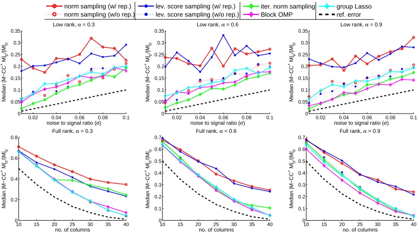
Figure 1: Selection error on Gaussian random matrices. Top row: low-rank plus noise inputs, s = k = 15; bottom row: full-rank inputs. The black dashed lines denote noise-to-signal ratio σ in the first row and kM−MkkF in the second row. α indicates the observation rate (i.e., the number of observed entries divided byn1n2, the total number of

matrix entries). All algorithms are run for 8 times on each data set and the median error is reported. We report the median instead of the mean because the performance of norm and leverage score sampling is quite variable.

5.3 Discussion on theoretical assumptions of block OMP and group Lasso

We discuss theoretical assumptions required for block OMP and group Lasso approaches. It should be noted that for the particular matrix column subset selection problem, neither Balzano et al. (2010a) or Bien et al. (2010) provides rigorous theoretical guarantee of ap-proximation error of the selected column subsets. However, it is informative to compare to typical assumptions that are used to analyze block OMP and group Lasso for regression problems in the existing literature (Yuan and Lin, 2006; Lounici et al., 2011). In most cases, certain “restricted eigenvalue” conditions on the design matrixX, which roughly cor-responds to a “weak correlation” condition among columns of a data matrix. This explains the worse performance of both methods on data sets that have highly correlated columns (e.g., many repeated columns), as we shown in later sections on experimental results.

6. Experiments

In this section we report experimental results on both synthetic and real-world data sets for our proposed column subset selection algorithms as well as other competitive methods. All algorithms are implemented in Matlab. To make fair comparisons, all input matrices

Mare normalized so that kMk2

norm sampling (w/ rep.) norm sampling (w/o rep.)

lev. score sampling (w/ rep.) lev. score sampling (w/o rep.)

iter. norm sampling Block OMP

group Lasso ref. error

0.02 0.04 0.06 0.08 0.1

0 0.1 0.2 0.3 0.4

noise to signal ratio (σ)

Median |M−CC

+ M|

F

/|M|

F

Low rank, α = 0.3

0.02 0.04 0.06 0.08 0.1

0 0.05 0.1 0.15 0.2 0.25 0.3 0.35

noise to signal ratio (σ)

Median |M−CC

+ M|

F

/|M|

F

Low rank, α = 0.6

0.02 0.04 0.06 0.08 0.1

0 0.05 0.1 0.15 0.2 0.25 0.3 0.35

noise to signal ratio (σ)

Median |M−CC

+ M|

F

/|M|

F

Low rank, α = 0.9

10 15 20 25 30 35 40

0 0.1 0.2 0.3 0.4

no. of columns

Median |M−CC

+ M|

F

/|M|

F

Full rank, α = 0.3

10 15 20 25 30 35 40

0 0.1 0.2 0.3 0.4 0.5

no. of columns

Median |M−CC

+ M|

F

/|M|

F

Full rank, α = 0.6

10 15 20 25 30 35 40

0 0.1 0.2 0.3 0.4

no. of columns

Median |M−CC

+ M|

F

/|M|

F

Full rank, α = 0.9

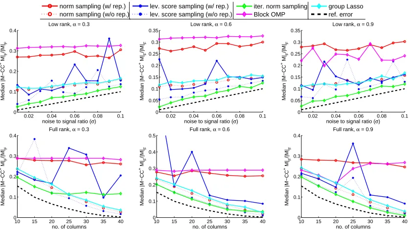
Figure 2: Selection error on matrices with coherent columns. Top row: low-rank plus noise inputs, s= k = 15; bottom row: full-rank inputs. α indicates the observation rate. The black dashed lines denote noise-to-signal ratio σ in the first row and kM−MkkF in the second row. All algorithms are run for 8 times on each data set and the median error is reported.

norm sampling (w/ rep.) norm sampling (w/o rep.)

lev. score sampling (w/ rep.) lev. score sampling (w/o rep.)

iter. norm sampling Block OMP

group Lasso ref. error

0 5 10 15 20 25 30 35

0.05 0.1 0.15 0.2 0.25 0.3 0.35 0.4

no. of repeated columns

Median |M−CC

+ M|

F

/|M|

F

α=0.3

0 5 10 15 20 25 30 35

0.05 0.1 0.15 0.2 0.25 0.3 0.35 0.4

no. of repeated columns

Median |M−CC

+ M|

F

/|M|

F

α=0.6

0 5 10 15 20 25 30 35

0.05 0.1 0.15 0.2 0.25 0.3 0.35 0.4

no. of repeated columns

Median |M−CC

+ M|

F

/|M|

F

α=0.9

Figure 3: Selection error on matrices with varying number of repeated columns. Both s

and kare set to 15 and the noise-to-signal ratioσ is set to 0.1. αindicates the observation rate. All algorithms are run for 8 times on each data set and the median error is reported.

6.1 Synthetic data sets

We first test the proposed algorithms on synthetic data sets. The input matrix has dimen-sion n1 =n2 =n= 50. To generate the synthetic data, we consider two different settings

listed below:

5 10 15 20 25 0.08 0.1 0.12 0.14 0.16 0.18 0.2

no. of columns

Averaging |M−CC

+ M|

F

2/|M|

F

2

α = 0.1, ε = 5%

norm sampling (w/ rep.) norm sampling (w/o rep.) lev. score sampling (w/ rep.) lev. score sampling (w/o rep.) iter. norm sampling

5 10 15 20 25

0.08 0.1 0.12 0.14 0.16 0.18

no. of columns

Averaging |M−CC

+ M|

F

2/|M|

F

2

α = 0.3, ε = 5%

norm sampling (w/ rep.) norm sampling (w/o rep.) lev. score sampling (w/ rep.) lev. score sampling (w/o rep.) iter. norm sampling

5 10 15 20 25

0.08 0.1 0.12 0.14 0.16 0.18

no. of columns

Averaging |M−CC

+ M|

F

2/|M|

F

2

α = 0.6, ε = 5%

norm sampling (w/ rep.) norm sampling (w/o rep.) lev. score sampling (w/ rep.) lev. score sampling (w/o rep.) iter. norm sampling

5 10 15 20 25

0.04 0.06 0.08 0.1 0.12 0.14

no. of columns

Averaging |M−CC

+ M|

F

2/|M|

F

2

α = 0.1, ε = 2%

norm sampling (w/ rep.) norm sampling (w/o rep.) lev. score sampling (w/ rep.) lev. score sampling (w/o rep.) iter. norm sampling

5 10 15 20 25

0.04 0.06 0.08 0.1 0.12 0.14

no. of columns

Averaging |M−CC

+ M|

F

2/|M|

F

2

α = 0.3, ε = 2%

norm sampling (w/ rep.) norm sampling (w/o rep.) lev. score sampling (w/ rep.) lev. score sampling (w/o rep.) iter. norm sampling

5 10 15 20 25

0.04 0.06 0.08 0.1 0.12 0.14

no. of columns

Averaging |M−CC

+ M|

F

2/|M|

F

2

α = 0.6, ε = 2%

norm sampling (w/ rep.) norm sampling (w/o rep.) lev. score sampling (w/ rep.) lev. score sampling (w/o rep.) iter. norm sampling

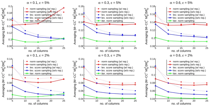
Figure 4: Selection error or sampling based algorithm on Hapmap phase2 data set. α

indicates the observation rate. Top row: top-k PCA captures 95% variance within each SNP window; bottom row: top-kPCA captures 98% variance within each SNP window.

0 0.2 0.4 0.6 0.8 1

0 2 4 6 8 10 12

Column no. (adjusted)

Column space leverage scores

Target rank (k) = 10

ε=5% ε=2%

0 0.2 0.4 0.6 0.8 1

0 1 2 3 4 5 6 7 8 9 10

Column no. (adjusted)

Column space leverage scores

Target rank (k) = 25

ε=5% ε=2%

Figure 5: Sorted column space leverage scores for differentεandksettings. For each setting 50 windows are picked at random and their leverage scores are plotted. Each plotted line is properly scaled along the X axis so that they have the same length even though actual window sizes vary.

generate a random Gaussian matrix B ∈ _Rn×k _{where k is the intrinsic rank and} then form the data matrix M as M = BB>. I.i.d. Gaussian noise R with Rij ∼ N(0, σ2) is then appended to the synthesized low-rank matrix. We remark that data matrices generated in this manner have both incoherent column and row space with high probability.

(a) The 512×512 8-bit gray scale Lena test image before compression.

(b) Norm sampling (without replacement). Selection errorkM−CC†MkF/kMkF = 0.106.

(c) Iterative norm sampling. Selection errorkM−CC†MkF/kMkF = 0.088.

(d) Approx. leverage score sampling (without replacement). kM−CC†MkF/kMkF = 0.103.

0 0.2 0.4 0.6 0.8 0

0.1 0.2 0.3 0.4 0.5 0.6

sampling probability α

|M−CC

+M|

F

k=10 k=20 k=30 k=40

0 0.02 0.04 0.06 0.08 0

0.1 0.2 0.3 0.4 0.5 0.6

rescaled sampling probability α/k

|M−CC

+M|

F

k=10 k=20 k=30 k=40

0 2 4 6 8

x 10−3 0

0.1 0.2 0.3 0.4 0.5 0.6

rescaled sampling probability α/k2

|M−CC

+M|

F

k=10 k=20 k=30 k=40

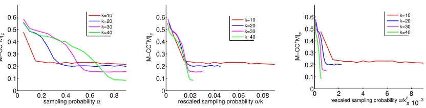
Figure 7: Selection error kM−CC†Mk_F for the iterative norm sampling algorithm as a function of α (left), α/k (middle) andα/k2 (right). Error curves plotted under 4 different rank (k) settings.

a column x from M uniformly at random. We then take ˜x = 10x and repeat the column for 5 times. As a result, the newly formed data matrix will have 5 identical columns with significantly higher norms compared to the other columns.

In Figure 1 we report the selection error kM−CC†Mk_F of proposed and baseline algorithms on random Gaussian matrices and in Figure 2 we report the same results on matrices with coherent columns. Results on both low-rank plus noise and high-rank inputs are reported. For low-rank matrices, both the intrinsic rank k and the number of selected columns s are set to 15. Each algorithm is run for 8 times on the same input and the median selection error is reported. For norm sampling and approximate leverage score sam-pling, we implement two variants: in thesampling with replacement scheme the algorithm samples each column from a sampling distribution (based on either norm or leverage score estimation) with replacement; while in thesampling without replacement scheme a column is never sampled twice. Note that all theoretical results in Section 3 are proved for sampling with replacement algorithms.

From Figure 1 we observe that all algorithms perform similarly, with the exception of two sampling with replacement algorithms and iterative norm sampling when both rank and missing rate are high. 3 For the latter case, we conjecture that the degradation of performance is due to inaccurate norm estimation of column residues; in fact, the iterative norm sampling only provably works when the input matrix has a low-rank plus noise struc-ture (see Theorem 2). On the other hand, when either the target rank or the missing rate is not too high iterative norm sampling works just as good; it is particularly competitive when the true rank of the input matrix is low (see the top row of Figure 1).

When the input matrix has coherent columns, as shown in Figure 2, it becomes easier to observe performance gaps among different algorithms. The block OMP algorithm com-pletely fails in such cases and the selection error for group Lasso also increases considerably. This is due to the fact that both algorithms observe matrix entries by sampling uniformly at random and hence could be poorly informed when the underlying matrix is highly co-herent. On the other hand, both leverage score sampling and iterative norm sampling are more robust to column coherence. The coherence among columns also makes the separation between norm sampling and volume sampling clearer in Figure 2. In particular, there is a

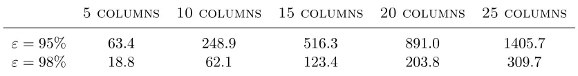
Table 2: Averaging SNP window sizes for differentεvalues and number of selected columns per window.

5 columns 10 columns 15 columns 20 columns 25 columns

ε= 95% 63.4 248.9 516.3 891.0 1405.7

ε= 98% 18.8 62.1 123.4 203.8 309.7

significant gap between the two sampling with replacement curves and the norm sampling algorithm degrades to its worst-case additive error bound (see Theorem 1). The gap be-tween the sampling without replacement curves is smaller since the coherent column is only repeated for 5 times in the design and so an algorithm can not be “too wrong” if it samples columns without replacement.

To further investigate how the proposed and baseline algorithms adapt to different levels of coherence, we report in Figure 3 the selection error on noisy low-rank matrices with varying number of repeated columns. Matrices with more repeated columns have higher coherence level. We can see that there is a clear separation of two groups of algorithms: the first group includes norm sampling, block OMP and group Lasso, whose error increases as the matrix becomes more coherent. Also, design matrix assumptions (e.g., restricted isometry) are violated for group Lasso. This suggests that these algorithms only have additive error bounds, or adapt poorly to column coherence of the underlying data matrix. On the other hand, the selection error of volume sampling and iterative norm sampling remains stable or slightly decreases. This is consistent with our theoretical results that both volume sampling and iterative norm sampling enjoy relative error bounds.

6.2 Application to tagging Single Nucleotide Polymorphisms (tSNPs) selection

We apply our proposed methods on real-world genetic data sets. We consider the tagging Single Nucleotide Polymorphisms (tSNP) selection task as described in (Ke and Cardon, 2003; Paschou et al., 2007). The task aims at selecting a small set of SNPs in human genes such that the selected SNPs (called tagging SNPs) capture the genetic information within a specific genome region. More specifically, given an n1×n2 matrix with each row

corresponding to the genome expression for an individual, we want to select k columns (typically k n2) corresponding to k tagging SNPs that best capture the entire SNP

matrix across different individuals. Matrix column subset selection methods have been successfully applied to the tSNP selection problem (Paschou et al., 2007).

consists of 89 rows (individuals) and 311,854 columns (SNPs). Each matrix entry has two lettersb1b2 describing a specific gene expression for an individual.

We follow the same step as described in (Javed et al., 2011) to preprocess the data. We first convert the raw data matrix into a numerical matrixMwith +1/0/-1 entries as follows: let B1 and B2 be the bases that appear for the jth SNP. Fix an individual i with its gene

expression b1b2. Ifb1b2=B1B1 thenMij is set to -1; else ifb1b2 =B2B2 thenMij is set 1; otherwise Mij is set to 0. We further split the SNPs into multiple consecutive “windows” so that within each window w the SVD reconstruction error kM(w)−M(_kw)k2

F/kM(w)k2F is no larger than ε with ε set to 5% and 2%. We refer the readers to Figure 1 in (Javed et al., 2011) for details of the preprocessing steps. Averaging window length (i.e., number of SNPs within each window) are shown in Table 2 for different k and ε settings. After preprocessing, column subset selection algorithms are performed for each SNP window and the selection error is averaged across all windows, as reported in Figure 4. The number of selected columns per window (k) ranges from 5 to 25 and the sampling budget α ranges from 10% to 60%.

In Figure 4 we observe that iterative norm sampling and approximate leverage score sampling outperform norm sampling by a large margin. This is because the truncated data matrix within each window is very close to an exact low-rank matrix and hence relative error algorithms achieve much better performance than additive error ones. In addition, approximate leverage score sampling significantly outperforms norm sampling under both the with replacement and without replacement schemes. This shows that the heterogeneity of human SNPs cannot be captured merely by their norms because the norm is simply the proportion of heterozygous within a population and provides little information about its importance across the entire chromosome. The spikiness of leverage score distribution is empirically verified in Figure 5. Finally, we remark that sampling without replacement is much better than sampling with replacement and should always be preferred in practice. We discuss this aspect in Section 7.5.

6.3 Application to column-based image compression

In this section we show how active sampling can be applied to column-based image com-pression without observing entire images. Given an image, we first actively subsample a small number of pixels from the original image. We then select a subset of columns based on the observed pixels and reconstruct the entire image by projecting each column to the space spanned by the selected column subsets.

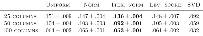
In Figure 6 we depicted the final compressed image as well as intermediate steps (e.g., subsampled pixels and selected columns) on the 512×512 8-bit gray scale Lena standard test image. We also report the mean and standard deviation of selection error across 10 runs under different settings of target column subset sizes in Table 3.