Multiclass Boosting for Weak Classifiers

Multiclass Boosting for Weak Classifiers

G ¨unther Eibl [email protected]

Karl–Peter Pfeiffer [email protected]

Department of Biostatistics University of Innsbruck

Sch¨opfstrasse 41, 6020 Innsbruck, Austria

Editor: Robert Schapire

Abstract

AdaBoost.M2 is a boosting algorithm designed for multiclass problems with weak base classifiers. The algorithm is designed to minimize a very loose bound on the training error. We propose two alternative boosting algorithms which also minimize bounds on performance measures. These performance measures are not as strongly connected to the expected error as the training error, but the derived bounds are tighter than the bound on the training error of AdaBoost.M2. In experiments the methods have roughly the same performance in minimizing the training and test error rates. The new algorithms have the advantage that the base classifier should minimize the confidence-rated error, whereas for AdaBoost.M2 the base classifier should minimize the pseudo-loss. This makes them more easily applicable to already existing base classifiers. The new algorithms also tend to converge faster than AdaBoost.M2.

Keywords: boosting, multiclass, ensemble, classification, decision stumps

1. Introduction

Most papers about boosting theory consider two-class problems. Multiclass problems can be either reduced to two-class problems using error-correcting codes (Allwein et al., 2000; Dietterrich and Bakiri, 1995; Guruswami and Sahai, 1999) or treated more directly using base classifiers for multi-class problems. Freund and Schapire (1996 and 1997) proposed the algorithm AdaBoost.M1 which is a straightforward generalization of AdaBoost using multiclass base classifiers. An exponential decrease of an upper bound of the training error rate is guaranteed as long as the error rates of the base classifiers are less than 1/2. For more than two labels this condition can be too restrictive for weak classifiers like decision stumps which we use in this paper. Freund and Schapire overcame this problem with the introduction of the pseudo-loss of a classifier h : X_×Y _→[0,1]:

εt=

1

2 1−ht(xi,yi) + 1 |Y_{| −}1_y

∑

i

ht(xi,y)

!

.

In the algorithm AdaBoost.M2, each base classifier has to minimize the pseudo-loss instead of the error rate. As long as the pseudo-loss is less than 1/2, which is easily reachable for weak base classifiers as decision stumps, an exponential decrease of an upper bound on the training error rate is guaranteed.

framework of Mason et al. (1998, 1999). Combined with ideas of Freund and Schapire (1996, 1997) we get an exponential bound on a performance measure which we call pseudo-loss error. The second algorithm was motivated by the attempt to make AdaBoost.M1 work for weak base classifiers. We introduce the maxlabel error rate and derive bounds on it. For both algorithms, the bounds on the performance measures decrease exponentially under conditions which are easy to fulfill by the base classifier. For both algorithms the goal of the base classifier is to minimize the confidence-rated error rate which makes them applicable for a wide range of already existing base classifiers.

Throughout this paper S=_{(xi,yi); i=1, . . . ,N)}denotes the training set where each xibelongs

to some instance or measurement space X and each label yiis in some label set Y . In contrast to the

two-class case, Y can have_|Y_{| ≥}2 elements. A boosting algorithm calls a given weak classification algorithm h repeatedly in a series of rounds t =1, . . . ,T . In each round, a sample of the original training set S is drawn according to the weighting distribution Dt and used as training set for the

weak classification algorithm h. Dt(i)denotes the weight of example i of the original training set

S. The final classifier H is a weighted majority vote of the T weak classifiers ht whereαt is the

weight assigned to ht. Finally, the elements of a set M that maximize and minimize a function f are

denoted arg max

m∈M f(m)and arg minm∈Mf(m)respectively.

2. Algorithm GrPloss

In this section we will derive the algorithm GrPloss. Mason et al. (1998, 1999) embedded Ad-aBoost in a more general theory which sees boosting algorithms as gradient descent methods for the minimization of a loss function in function space. We get GrPloss by applying the gradient descent framework especially for minimizing the exponential pseudo-loss. We first consider slightly more general exponential loss functions. Based on the gradient descent framework, we derive a gradient descent algorithm for these loss functions in a straight forward way in Section 2.1. In contrast to the general framework, we can additionally derive a simple update rule for the sampling distribution as it exists for AdaBoost.M1 and AdaBoost.M2. Gradient descent does not provide a special choice for the “step size”αt. In Section 2.2, we define the pseudo-loss error and deriveαt by minimization

of an upper bound on the pseudo-loss error. Finally, the algorithm is simplified for the special case of decision stumps as base classifiers.

2.1 Gradient Descent for Exponential Loss Functions

First we briefly describe the gradient descent framework for the two-class case with Y=_{−1,+1}. As usual a training set S=_{(xi,yi); i=1, . . . ,N)} is given. We are considering a function space

F

H

f(x;~α,~β) =

T

∑

t=1

αtht(x;βt), ht: X → {±1}

with~α= (α1, . . . ,αT)∈RT, ~β= (β1, . . . ,βT)and ht ∈

H

ht therefore~αand~βuniquely determine f . We choose a loss function

where for example the choice of l(f(x),y) =e−y f(x)leads to

L(f) = 1

N

N

∑

i=1 eyif(xi)_.

The goal is to find f∗=arg min

f∈FL(f).

The gradient in function space is defined as:

∇L(f)(x):=∂L(f+e1x)

∂e |e=0=elim→0

L(f+e1x)−L(f)

e

where for two arbitrary tuples v and ˜v we denote

1v(v˜) =

1 v˜=v

0 v˜₆=v.

A gradient descent method always makes a step in the “direction” of the negative gradient−∇L(f)(x). However₋∇L(f)(x)is not necessarily an element of

F

F

which is as parallel to₋∇L(f)(x)as possible. Therefore we need an inner product_h,_i:

F

F

hf,f˜_i= 1

N

N

∑

i=1

f(xi)f˜(xi).

This inner product measures the agreement of f and ˜f on the training set. Using this inner product we can set

βt:=arg max

β h−∇L(ft−1),h(·;β)i

and ht:=h(·;βt). The inequalityh−∇L(ft₋1),h(βt)i ≤0 means that we can not find a good

“direc-tion” h(βt), so the algorithm stops, when this happens. The resulting algorithm is given in Figure 1.

————————————————————————————————– Input: training set S, loss function l, inner product_h,_i:

F

F

Loop: while_h−∇L(ft−1),h(βt)i >0

• βt:=arg max

β h−∇L(ft−1),h(β)i • αt:=arg min_α (L(ft−1+αht(βt)))

• ft =ft−1+αtht(βt)

Output: ft,L(ft)

————————————————————————————————–

Figure 1: Algorithm gradient descent in function space

object with measurements x has the label y. We denote the set of possible classifiers with

F

F

hf,fˆ_i:= 1

N

N

∑

i=1 |Y|

∑

y=1

f(xi,y)fˆ(xi,y),

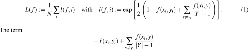
which is a straightforward generalization of the definition for the two-class case. The goal of the classification algorithm GrPloss is to minimize the special loss function

L(f):= 1

N

∑

"

1

2 1−f(xi,yi) +_y

∑

i

f(xi,y)

|Y_{| −}1

!#

. (1)

The term

−f(xi,yi) +

∑

f(xi,y)

|Y_{| −}1

compares the confidence to label the example xicorrectly with the mean confidence of choosing one

of the wrong labels. Now we consider slightly more general exponential loss functions

l(f,i) =exp[v(f,i)] with exponent₋loss v(f,i) =v0+

∑

y

vy(i)f(xi,y),

where the choice

v0= 1

2 and vy(i) =

(

−1

2 y=yi

1

2(|Y|−1) y6=yi

leads to the loss function (1). This choice of the loss function leads to the algorithm given in Fig-ure 2. The properties summarized in Theorem 1 can be shown to hold on this algorithm.

————————————————————————————– Input: training set S, maximum number of boosting rounds T

Initialisation: f0:=0, t :=1,∀i : D1(i):=_N1. Loop: For t=1, . . . ,T do

• ht=arg min

h ∑iDt(i)v(h,i)

• If∑iDt(i)v(ht,i) ≥v0: T :=t−1, goto output. • Chooseαt.

• Update ft = ft−1+αtht and Dt+1(i) =_Z1_tDt(i)l(αtht,i)

Output: fT,L(fT)

————————————————————————————–

Theorem 1 For the inner product

hf,h_i= 1

N

N

∑

i=1 |Y_|

∑

y=1

f(xi,y)h(xi,y)

and any exponential loss functions l(f,i)of the form

l(f,i) =exp[v(f,i)] with v(f,i) =v0+

∑

y

vy(i)f(xi,y)

where v0and vy(i)are constants, the following statements hold:

(i) The choice of ht that maximizes the projection on the negative gradient

ht=arg max

h h−∇L(ft−1),hi

is equivalent to that minimizing the weighted exponent-loss

ht =arg min

h

∑

with respect to the sampling distribution

Dt(i):=

l(ft−1,i) ∑

i0 l(ft−1,i

0₎ =

l(ft−1,i) Z_t0₋₁ . (ii) The stopping criterion of the gradient descent method

h−∇L(ft−1),h(βt)i ≤0

leads to a stop of the algorithm, when the weighted exponent-loss gets positive

∑

i

Dt(i)v(ht,i)≥v0.

(iii) The sampling distribution can be updated in a similar way as in AdaBoost using the rule

Dt+1(i) = 1 Zt

Dt(i)l(αtht,i),

where we define Zt as a normalization constant

Zt:=

∑

Dt(i)l(αtht,i),

which ensures that the update Dt+1is a distribution.

In contrast to the general framework, the algorithm uses a simple update rule for the sampling distribution as it exists for the original boosting algorithms. Note that the algorithm does not specify the choice of the step sizeαt, because gradient descent only provides an upper bound onαt. We

Proof. The proof basically consists of three steps: the calculation of the gradient, the choice for base classifier ht together with the stopping criterion and the update rule for the sampling distribution.

(i) First we calculate the gradient, which is defined by

∇L(f)(x,y):=lim

k→0

L(f+k1(x,y))−L(f)

k

for 1_(x,y)(x0,y0) =n1₀ (_(xx,_,y_y)=(₎ x0,y0)

6

=(x0_,y0₎.

So we get for x=xi:

L(f+k1xiy) =

1 Nexp

"

v0+

∑

y0

vy0(i)f(x_i,y0) +kv_y(i) #

= 1

Nl(f,i)e

kvy(i)_.

Substitution in the definition of∇L(f)leads to

∇L(f)(xi,y) =lim k→0

l(f,i)(ekvy(i)₋₁₎

k =l(f,i)vy(i).

Thus

∇L(f)(x,y) =

0 x₆=xi

l(f,i)vy(i) x=xi

. (2)

Now we insert (2) into_h−∇L(ft−1),htiand get

h−∇L(ft₋1),hti=−

1

N

∑

∑

N

∑

Dt(i):=Ct₋1l(ft₋1,i), (4) we can write (3) as

h−∇L(ft−1),hti=−

1 Ct−1N

∑

Dt(i)(v(h,i)−v0) =− 1 Ct−1N

∑

Dt(i)v(h,i)−v0

!

. (5)

Since we require Ct₋1to be positive, we get the choice of ht of the algorithm

ht =arg max

h h−∇L(ft−1),hi=arg minh

∑

(ii) One can verify the stopping criterion of Figure 2 from (5)

h−∇L(ft₋1),hti ≤0⇔

∑

Dt(i)v(ht,i) ≥v0.

(iii) Finally, we show that we can calculate the update rule for the sampling distribution D.

Dt+1(i) = Ctl(ft,i) =Ctl(ft−1+αtht,i)

= Ctl(ft−1,i)l(αtht,i) =

Ct

Ct₋1

This means that the new weight of example i is a constant multiplied with Dt(i)l(αtht,i). By

com-paring this equation with the definition of Zt we can determine Ct

Ct =

Ct−1 Zt

.

Since l is positive and the weights are positive one can show by induction, that also Ct is positive,

which we required before.

2.2 Choice ofαt and Resulting Algorithm GrPloss

The algorithm above leaves the step lengthαt, which is the weight of the base classifier ht,

unspec-ified. In this section we define the pseudo-loss error and derive αt by minimization of an upper

bound on the pseudo-loss error.

Definition: A classifier f : X_×Y _→Rmakes a pseudo-loss error in classifying an example x with label k, if

f(x,k)< 1

|Y_{| −}1_y

∑

plerr := 1

N

N

∑

i=1

I f(xi,yi)<

1 |Y_{| −}1_y

∑

i

f(xi,y)

!

.

The pseudo-loss error counts the proportion of elements in the training set for which the confi-dence f(x,k) in the right label is smaller than the average confidence in the remaining labels

∑

y6=k

f(x,y)/(_|Y_{| −}1). Thus it is a weak measure for the performance of a classifier in the sense that it can be much smaller than the training error.

Now we consider the exponential pseudo-loss. The constant term of the pseudo-loss leads to a constant factor which can be put into the normalizing constant. So with the definition

u(f,i):= f(xi,yi)−

1 |Y_{| −}1_y

∑

i

f(xi,y)

the update rule can be written in the shorter form

Dt+1(i) = 1 Zt

Dt(i)e−αtu(ht,i)/2,with Zt := N

∑

i=1

Dt(i)e−αtu(ht,i)/2.

We present our next algorithm, GrPloss, in Figure 3, which we will derive and justify in what follows.

(i) Similar to Schapire and Singer (1999) we first bound plerr by the product of the normalization constants

plerr_≤

T

∏

t=1

Zt. (6)

To prove (6), we first notice that

plerr_≤ 1 N

∑

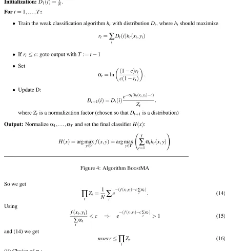
————————————————————————————————– Input: training set S=_{(x1,y1), . . . ,(xN,yN); xi∈X,yi∈Y},

Y=_{1, . . . ,_|Y_|}, weak classification algorithm with output h : X_×Y_→[0,1]

Optionally T : maximal number of boosting rounds

Initialization: D1(i) =_N1. For t=1, . . . ,T :

• Train the weak classification algorithm ht with distribution Dt, where ht should maximize

Ut :=∑iDt(i)u(ht,i).

• If Ut ≤0: goto output with T :=t−1

• Set

αt =ln

1+Ut

1₋Ut

.

• Update D:

Dt+1(i) = 1 Zt

Dt(i)e−αtu(ht,i)/2.

where Zt is a normalization factor (chosen so that Dt+1is a distribution) Output: final classifier H(x):

H(x) =arg max

y∈Y f(x,y) =arg maxy∈Y T

∑

t=1

αtht(x,y)

!

————————————————————————————————–

Figure 3: Algorithm GrPloss

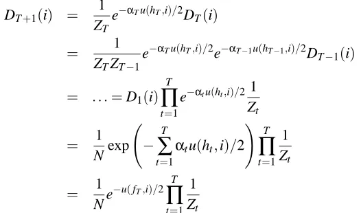
Now we unravel the update rule

DT+1(i) = 1 ZT

e−αTu(hT,i)/2_D

T(i)

= 1

ZTZT−1

e−αTu(hT,i)/2_e−αT−1u(hT−1,i)/2_D

T₋1(i)

= . . .=D1(i)

T

∏

t=1

e−αtu(ht,i)/2 1

Zt

= 1

Nexp −

T

∑

t=1

αtu(ht,i)/2

!

T

∏

t=1 1 Zt

= 1

Ne

−u(fT,i)/2

T

∏

t=1 1 Zt

where the last equation uses the property that u is linear in h. Since

1=

∑

i

DT+1(i) =

∑

i

1 Ne

−u(fT,i)/2

∏

we get Equation (6) by using (7) and the equation above

plerr_≤ 1 N

∑

−u(fT,i)/2₌

T

∏

t=1 Zt.

(ii) Derivation ofαt:

Now we deriveαt by minimizing the upper bound (6). First, we plug in the definition of Zt

T

∏

t=1 Zt=

T

∏

t=1

∑

Dt(i)e−αtu(ht,i)/2

!

.

Now we get an upper bound on this product using the convexity of the function e−αtu_between−1

and +1 (from h(x,y)_∈[0,1]it follows that u_∈[₋1,+1]) for positiveαt: T

∏

t=1 Zt ≤

T

∏

t=1

∑

Dt(i)

1

2[(1−u(ht,i))e +1

2αt_{+ (1+u(h}

t,i))e−

1 2αt_]

!

. (8)

Now we chooseαt in order to minimize this upper bound by setting the first derivative with respect

toαt to zero. To do this, we define

Ut:=

∑

Dt(i)u(ht,i).

Since eachαt occurs in exactly one factor of the bound (8) the result forαt only depends on Ut and

not on Us, s6=t, more specifically

αt =ln

1+Ut

1₋Ut

.

Note that Ut has its values in the interval[−1,1], because ut∈[−1,+1]and Dt is a distribution.

(iii) Derivation of the upper bound of the theorem:

Now we substituteαtback in (8) and get after some straightforward calculations

T

∏

t=1 Zt ≤

T

∏

t=1

q

1₋Ut2.

Using the inequality√1₋x_≤(1₋1₂x)_≤e−x/2 for x_∈[0,1]we can get an exponential bound on ∏tZt

T

∏

t=1

Zt≤exp

"

T

∑

t=1 −U_t2/2

#

.

If we assume that each classifier ht fulfills Ut ≥δ, we finally get T

∏

t=1

Zt ≤e−δ

2_T/2

.

(iv) Stopping criterion:

The stopping criterion of the slightly more general algorithm directly results in the new stopping criterion to stop, when Ut ≤0. However, note that the bound depends on the square of Ut instead of

We summarize the foregoing argument as a theorem.

Theorem 2 If for all base classifiers ht: X×Y →[0,1]of the algorithm GrPloss given in Figure 3

Ut :=

∑

Dt(i)u(ht,i)≥δ

holds forδ>0 then the pseudo-loss error of the training set fulfills

plerr_≤

T

∏

t=1

q

1₋Ut2≤e−δ

2_T/2

. (9)

2.3 GrPloss for Decision Stumps

So far we have considered classifiers of the form h : X_×Y _→[0,1]. Now we want to consider base classifiers that have additionally the normalization property

∑

y_∈Y

h(x,y) =1 (10)

which we did not use in the previous section for the derivation ofαt. The decision stumps we used

in our experiments find an attribute a and a value v which are used to divide the training set into two subsets. If attribute a is continuous and its value on x is at most v then x belongs to the first subset; otherwise x belongs to the second subset. If attribute a is categorical the two subsets correspond to a partition of all possible values of a into two sets. The prediction h(x,y)is the proportion of examples with label y belonging to the same subset as x. Since proportions are in the interval[0,1]

and for each of the two subsets the sum of proportions is one our decision stumps have both the former and the latter property (10). Now we use these properties to minimize a tighter bound on the pseudo-loss error and further simplify the algorithm.

(i) Derivation ofαt:

To getαt we can start with

plerr_≤

T

∏

t=1 Zt=

T

∏

t=1

∑

Dt(i)e−αtu(ht,i)/2

!

which was derived in part (i) of the proof of the previous section. First, we simplify u(h,i)using the normalization property and get

u(h,i) = |Y|

|Y_{| −}1h(xi,yi)− 1

|Y_{| −}1 (11)

In contrast to the previous section, u(h,i)_∈[₋ 1

|Y|−1,1]for h(xi,yi)∈[0,1], which we will take into account for the convexity argument:

plerr_≤

T

∏

t=1

N

∑

i=1 Dt(i)

h(xi,yi)e−αt/2+ (1−ht(xi,yi))eαt/(2(|Y|−1))

Setting the first derivative with respect toαt to zero leads to

αt =

2(_|Y_{| −}1)

|Y_| ln

(_|Y_{| −}1)rt

1₋rt

,

where we defined

rt:= N

∑

i=1

Dt(i)ht(xi,yi).

(ii) Upper bound on the pseudo-loss error: Now we plugαt in (12) and get

plerr_≤

T

∏

t=1 rt

1₋rt

rt(|Y| −1)

(|Y|−1)/|Y|

+ (1₋rt)

rt(|Y| −1)

1−rt

1/|Y|!

. (13)

(iii) Stopping criterion:

As expected for rt =1/|Y| the corresponding factor is 1. The stopping criterion Ut ≤0 can be

directly translated into rt ≥1/|Y|. Looking at the first and second derivative of the bound one can

easily verify that it has a unique maximum at rt =1/|Y|. Therefore, the bound drops as long as

rt >1/|Y|. Note again that since rt=1/|Y|is a unique maximum we get a formal decrease of the

bound even when rt>1/|Y|.

(iv) Update rule:

Now we simplify the update rule using (11) and insert the new choice ofαt and get

Dt+1(i) = Dt(i)

Zt

e−α˜t(ht(xi,yi)−1/|Y|) _for α_˜

t :=ln

(_|Y_{| −}1)rt

1−rt

Also the goal of the base classifier can be simplified, because maximizing Ut is equivalent to

maxi-mizing rt.

We will see in the next section, that the resulting algorithm is a special case of the algorithm BoostMA of the next chapter with c=1/_|Y_|.

3. BoostMA

The aim behind the algorithm BoostMA was to find a simple modification of AdaBoost.M1 in order to make it work for weak base classifiers. The original idea was influenced by a frequently used argument for the explanation of ensemble methods. Assuming that the individual classifiers are uncorrelated, majority voting of an ensemble of classifiers should lead to better results than using one individual classifier. This explanation suggests that the weight of classifiers that perform better than random guessing should be positive. This is not the case for AdaBoost.M1. In AdaBoost.M1 the weight of a base classifierαis a function of the error rate, so we tried to modify this function so that it gets positive, if the error rate is less than the error rate of random guessing. The resulting classifier AdaBoost.M1W showed good results in experiments (Eibl and Pfeiffer, 2002). Further theoretical considerations led to the more elaborate algorithm which we call BoostMA which uses confidence-rated classifiers and also compares the base classifier with the uninformative rule.

X×Y →[0,1] performs worse than the uninformative or what we call the maxlabel rule. The maxlabel rule labels each instance as the most frequent label. As a confidence-rated classifier, the uninformative rule has the form

maxlabel rule : X_×Y _→[0,1]: h(x,y):=Ny

N,

where Nyis the number of instances in the training set with label y. So it seems natural to investigate

a modification where the update of the sampling distribution has the form

Dt+1(i) =Dt(i)

e−αt(ht(xi,yi)−c)

Zt

,with Zt := N

∑

i=1

Dt(i)e−αt(ht(xi,yi)−c),

where c measures the performance of the uninformative rule. Later we will set

c :=

∑

y∈Y

Ny

N

2

and justify this setting. But up to that point we let the choice of c open and just require c_∈(0,1). We now define a performance measure which plays the same role as the pseudo-loss error.

Definition 1 Let c be a number in(0,1). A classifier f : X_×Y _→[0,1]makes a maxlabel error in classifying an example x with label k, if

f(x,k)<c.

The maxlabel error for the training set is called mxerr:

mxerr := 1

N

N

∑

i=1

I(f(xi,yi)<c).

The maxlabel error counts the proportion of elements of the training set for which the confidence f(x,k)in the right label is smaller than c. The number c must be chosen in advance. The higher c is, the higher is the maxlabel error for the same classifier f ; therefore to get a weak error measure we set c very low. For BoostMA we choose c as the accuracy for the uninformative rule. When we use decision stumps as base classifiers we have the property h(x,y)_∈[0,1]. By normalizingα1, . . . ,αT,

so that they sum to one, we ensure f(x,y)_∈[0,1](Equation 15).

We present the algorithm BoostMA in Figure 4 and in what follows we justify and establish some properties about it. As for GrPloss the modus operandi consists of finding an upper bound on mxerr and minimizing the bound with respect toα.

(i) Bound of mxerr in terms of the normalization constants Zt:

Similar to the calculations used to bound the pseudo-loss error we begin by bounding mxerr in terms of the normalization constants Zt: We have

1 =

∑

i

Dt+1(i) =

∑

i

Dt(i)

e−αt(ht(xi,yi)−c)

Zt

=. . .

= 1

∏

s

Zs

1 N

∑

t

∏

s=1

e−αs(hs(xi,yi)−c)₌ 1

∏

s

Zs

1 N

∑

−(f(xi,yi)−c∑ sαs

)

————————————————————————————————— Input: training set S=_{(x1,y1), . . . ,(xN,yN); xi∈X,yi∈Y},

Y=_{1, . . . ,_|Y_|}, weak classification algorithm of the form h : X_×Y _→[0,1]. Optionally T : number of boosting rounds

Initialization: D1(i) =_N1. For t=1, . . . ,T :

• Train the weak classification algorithm ht with distribution Dt, where ht should maximize

rt=

∑

Dt(i)ht(xi,yi)

• If rt≤c: goto output with T :=t−1

• Set

αt=ln

(1−c)rt

c(1₋rt)

.

• Update D:

Dt+1(i) =Dt(i)

e−αt(ht(xi,yi)−c)

Zt

.

where Zt is a normalization factor (chosen so that Dt+1is a distribution) Output: Normalizeα1, . . . ,αT and set the final classifier H(x):

H(x) =arg max

y∈Y f(x,y) =arg maxy∈Y T

∑

t=1

αtht(x,y)

!

—————————————————————————————————

Figure 4: Algorithm BoostMA

So we get

∏

t

Zt =

1 N

∑

−(f(xi,yi)−c∑

t αt). ₍₁₄₎

Using

f(xi,yi)

∑

t αt

<c _⇒ e−(f(xi,yi)−c∑t αt

)

>1 (15)

and (14) we get

mxerr_≤

∏

t

Zt. (16)

(ii) Choice ofαt:

Now we bound∏

t

Zt and then we minimize it, which leads us to the choice ofαt. First we use the

definition of Zt and get

∏

t

Zt=

∏

∑

Dt(i)e−αt(ht(xi,yi)−c)

!

Now we use the convexity of e−αt(ht(xi,yi)−c)_{for h}

t(xi,yi)between 0 and 1 and the definition

rt:=

∑

Dt(i)ht(xi,yi)

and get

mxerr _≤

∏

t

∑

Dt(i)

ht(xi,yi)e−αt(1−c)+ (1−ht(xi,yi))eαtc

=

∏

t

rte−αt(1−c)+ (1−rt)eαtc

.

We minimize this by setting the first derivative with respect toαt to zero, which leads to

αt =ln

(1₋c)rt

c(1₋rt)

.

(iii) First bound on mxerr:

To get the bound on mxerr we substitute our choice forαt in (17) and get

mxerr_≤

∏

t

(1₋c)rt

c(1₋rt)

c

∑

i

Dt(i)

c(1₋rt)

(1₋c)rt

ht(xi,yi)!

. (18)

Now we bound the termc(1−rt)

(1−c)rt

ht(xi,yi)

by use of the inequality

xa_≤1₋a+ax for x_≥0 and a_∈[0,1],

which comes from the convexity of xafor a between 0 and 1 and get

c(1₋rt)

(1₋c)rt

ht(xi,yi)

≤1₋ht(xi,yi) +ht(xi,yi)

c(1₋rt)

(1₋c)rt

.

Substitution in (18) and simplifications lead to

mxerr_≤

∏

t

r_tc(1₋rt)1−c

(1₋c)1−c_cc

. (19)

The factors of this bound are symmetric around rt=c and take their maximum of 1 there. Therefore

if rt >c is valid the bound on mxerr decreases.

(iv) Exponential decrease of mxerr:

To prove the second bound we set rt=c+δwithδ∈(0,1−c)and rewrite (19) as

mxerr_≤

∏

t

1₋ δ

1₋c

1−c

1+δ

c

c

.

We can bound both terms using the binomial series: all terms of the series of the first term are negative, we stop after the terms of first order and get

1₋ δ

1₋c

1−c

The series of the second term has both positive and negative terms, we stop after the positive term of first order and get

1+δ

c

c

≤1+δ.

Thus

mxerr_≤

∏

t

(1₋δ2).

Using 1+x_≤exfor x_≤0 leads to

mxerr_≤e−δ2T.

We summarize the foregoing argument as a theorem.

Theorem 3 If all base classifiers htwith ht(x,y)∈[0,1]fulfill

rt:=

∑

Dt(i)ht(xi,yi)≥c+δ

forδ_∈(0,1₋c) (and the condition c_∈(0,1))then the maxlabel error of the training set for the algorithm in Figure 4 fulfills

mxerr_≤

∏

t

rc_t(1₋rt)1−c

(1−c)1−c_cc

≤e−δ2T. (20)

Remarks: 1.) Choice of c for BoostMA: since we use confidence-rated base classification algorithms we choose the training accuracy for the confidence-rated uninformative rule for c, which leads to

c= 1

N

N

∑

i=1 Nyi

N =

1 N

∑

∑

i=y

Ny

N =_y

∑

Ny

N

2

. (21)

2.) For base classifiers with the normalization property (10) we can get a simpler expression for the pseudo-loss error. From

∑

y₆=k

f(x,y) =

∑

y₆=k

∑

αtht(x,y) =

∑

αt(1−ht(x,k)) =

∑

αt−f(x,k)

we get

f(x,k)< 1

|Y_{| −}1_y

∑

6

=k

f(x,y) _⇔ f(x,k)

∑

t αt

< 1

|Y_|. (22)

That means that if we choose c=1/_|Y_|for BoostMA the maxlabel error is the same as the pseudo-loss error. For the choice (21) of c this is the case when the group proportions are balanced, because then

c=

∑

y∈Y

Ny

N

2

=

∑

y∈Y

1 |Y_|

2

=_|Y_| 1 |Y_|2 =

1 |Y_|.

For this choice of c the update rule of the sampling distribution for BoostMA gets

Dt+1(i) = Dt(i)

Zt

e−αt(ht(xi,yi)−1/|Y|) _and α

t=ln

(_|Y_{| −}1)rt

1₋rt

which is just the same as the update rule GrPloss for decision stumps. Summarizing these two re-sults we can say that for base classifiers with the normalization property, the choice (21) for c of BoostMA and data sets with balanced labels, the two algorithms GrPloss and BoostMA and their error measures are the same.

3.) In contrast to GrPloss the algorithm does not change when the base classifier additionally fulfills the normalization property (10) because the algorithm only uses ht(xi,yi).

4. Experiments

In our experiments we focused on the derived bounds and the practical performance of the algo-rithms.

4.1 Experimental Setup

To check the performance of the algorithms experimentally we performed experiments with 12 data sets, most of which are available from the UCI repository (Blake and Merz, 1998). To get reliable estimates for the expected error rate we used relatively large data sets consisting of about 1000 cases or more. The expected classification error was estimated either by a test error rate or 10-fold cross-validation. A short overview of the data sets is given in Table 1.

Database N ]Labels ]Variables Error Estimation Labels

car * 1728 4 6 10-CV unbalanced

digitbreiman 5000 10 7 test error balanced

letter 20000 26 16 test error balanced

nursery * 12960 4 8 10-CV unbalanced

optdigits 5620 10 64 test error balanced

pendigits 10992 10 16 test error balanced

satimage * 6435 6 34 test error unbalanced

segmentation 2310 7 19 10-CV balanced

waveform 5000 3 21 test error balanced

vehicle 846 4 18 10-CV balanced

vowel 990 11 10 test error balanced

yeast * 1484 10 9 10-CV unbalanced

Table 1: Properties of the databases

For all algorithms we used boosting by resampling with decision stumps as base classifiers. We used AdaBoost.M2 by Freund and Schapire (1997), BoostMA with c=∑_y∈Y(Ny/N)2 and the

algorithm GrPloss for decision stumps of Section 2.3 which corresponds to BoostMA with c=

1/_|Y_|. For only four databases the proportions of the labels are significantly unbalanced so that GrPloss and BoostMA should have greater differences only for these four databases (marked with a *). As discussed by Bauer and Kohavi (1999) the individual sampling weights Dt(i)can get very

We also set a maximum number of 2000 boosting rounds to stop the algorithm if the stopping criterion is not satisfied.

4.2 Results

The experiments have two main goals. From the theoretical point of view one is interested in the derived bounds. For the practical use of the algorithms, it is important to look at the training and test error rates and the speed of the algorithms.

4.2.1 DERIVEDBOUNDS

First we look at the bounds on the error measures. For the algorithm AdaBoost.M2, Freund and Schapire (1997) derived the upper bound

(_|Y_{| −}1)2T−1

T

∏

t=1

p

εt(1−εt) (23)

on the training error. We have three different bounds on the pseudo-loss error of Grploss: the term

∏

t

Zt (24)

which was derived in the first part of the proof of Theorem 2, the tighter bound (9) of Theorem 2 and the bound (13) for the special case of decision stumps as base classifiers. In Section 3, we derived two upper bounds on the maxlabel error for BoostMA: term (24) and the tighter bound (20) of Theorem 3.

For all algorithms their respective bounds hold for all time steps and for all data sets. Bound (23) on the training error of AdaBoost.M2 is very loose – it even exceeds 1 for eight of the 12 data sets, which is possible due to the factor_|Y_{| −}1 (Table 2). In contrast to the bound on the training error of AdaBoost.M2, the bounds on the pseudo-loss error of GrPloss and the maxlabel error of BoostMA are below 1 for all data sets and all boosting rounds. In that sense, they are tighter than the bounds on the training error of AdaBoost.M2.

As expected, bound (13) derived for the special case of decision stumps as base classifiers on the pseudo-loss error is smaller than bound (9) of Theorem 2 which doesn’t use the normalization property (10) of the decision stumps.

For both GrPloss and BoostMA, bound (24) is the smallest bound since it contains the fewest approximations. For BoostMA, term (24) is a bound on the maxlabel error and for GrPloss term (24) is a bound on the pseudo-loss error. For unbalanced data sets, the maxlabel error is the “harder” error measure than the pseudo-loss error, so for these data sets bound (24) is higher for BoostMA than for GrPloss. For balanced data sets the maxlabel error and the pseudo-loss error are the same. Bound (9) for GrPloss is higher for these data sets than bound (20) of BoostMA. This suggests that bound (9) for GrPloss could be improved by more sophisticated calculations.

4.2.2 COMPARISON OF THEALGORITHMS

AdaBoost.M2 GrPloss BoostMA

training error [%] pseudo-loss error [%] maxlabel error [%]

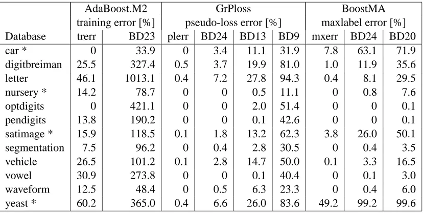
Database trerr BD23 plerr BD24 BD13 BD9 mxerr BD24 BD20

car * 0 33.9 0 3.4 11.1 31.9 7.8 63.1 71.9

digitbreiman 25.5 327.4 0.5 3.7 19.9 81.0 1.0 11.9 35.6

letter 46.1 1013.1 0.4 7.2 27.8 94.3 0.4 8.1 29.5

nursery * 14.2 78.7 0 0 0.5 11.1 0 0.8 7.6

optdigits 0 421.1 0 0 2.0 51.4 0 0 0.1

pendigits 13.8 190.2 0 0 0.1 42.6 0 0 0.1

satimage * 15.9 118.5 0.1 1.8 13.2 62.3 3.8 26.0 50.1

segmentation 7.5 96.2 0 0.4 2.8 30.5 0 0.4 3.5

vehicle 26.5 101.2 0.1 2.8 14.7 50.0 0.1 3.3 16.5

vowel 30.9 273.8 0 0 0.1 40.4 0 0.1 3.0

waveform 12.5 48.4 0 0.5 6.3 23.3 0 0.4 6.0

yeast * 60.2 365.0 0.4 6.6 26.0 83.6 49.2 99.2 99.6

Table 2: Performance measures and their bounds in percent at the boosting round with minimal training error. trerr, BD23: training error of AdaBoost and its bound (23); plerr, BD24 ,BD13 ,BD9: pseudo-loss error of GrPloss and its bounds (24), (13) and (9); mxerr, BD24, BD20: maxlabel error of BoostMA and its bounds (24) and (20).

all error rates at the boosting round with minimal training error rate as was done by Eibl and Pfeiffer (2002).

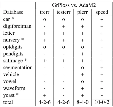
First we look at the minimum achieved training and test error rates. The theory suggests Ad-aBoost.M2 to work best in minimizing the training error. However, GrPloss seems to have roughly the same performance with maybe AdaBoost.M2 leading by a slight edge (Tables 3 and 4, Figure 5). The difference in the training error mainly carries over to the difference in the test error. Only for the data sets digitbreiman and yeast do the training and the test error favor different algorithms (Table 4). Both the training and the test error favor AdaBoost.M2 for six data sets and GrPloss for four data sets with two draws (Table 4).

While GrPloss and AdaBoost.M2 were quite close for the training and test error rates, this is not the case for the pseudo-loss error. Here, GrPloss is the clear winner against AdaBoost.M1 with eight wins and four draws (Table 4). The reason for this might be the fact that bound (13) on the pseudo-loss error of GrPloss is tighter than bound (23) on the training error of AdaBoost.M2 (Table 2). For the data set nursery, bound (13) on the pseudo-loss error of GrPloss (0.5%) is smaller than the pseudo-loss error of AdaBoost.M2 (1.9%). So for this data set, bound (13) can explain the superiority of GrPloss in minimizing the pseudo-loss error.

training error test error

Database AdaM2 GrPloss BoostMA AdaM2 GrPloss BoostMA

car * 0 0 7.75 0 0 7.75

digitbreiman 25.49 25.63 25.63 27.51 27.13 27.38

letter 46.07 40.02 40.14 47.18 41.70 41.70

nursery * 14.16 12.37 12.63 14.27 12.35 12.67

optdigits 0 0 0 0 0 0

pendigits 13.82 17.17 17.20 18.61 20.44 20.75

satimage * 15.85 15.69 16.87 18.25 17.80 18.90

segmentation 7.49 9.05 8.90 8.40 9.31 9.48

vehicle 26.46 30.15 30.19 35.34 38.16 36.87

vowel 30.87 41.67 42.23 54.33 67.32 67.32

waveform 12.45 14.55 14.49 16.63 18.17 17.72

yeast * 60.18 59.31 60.61 60.65 61.99 62.47

Table 3: Training and test error at the boosting round with minimal training error; bold and italic numbers correspond to high(>5%) and medium(>1.5%) differences to the smallest of the three error rates

GrPloss vs. AdaM2

Database trerr testerr plerr speed

car * o o o +

digitbreiman - + + +

letter + + + +

nursery * + + + +

optdigits o o o

-pendigits - - + +

satimage * + + + +

segmentation - - o +

vehicle - - + +

vowel - - o +

waveform - - + +

yeast * + - +

-total 4-2-6 4-2-6 8-4-0 10-0-2

Table 4: Comparison of GrPloss with AdaBoost.M2: win-loss-table for the training error, test error, pseudo-loss error and speed of the algorithm (+/o/-: win/draw/loss for GrPloss)

1 10 100 1000 10000 0

0.05 0.1

car

1 10 100 1000 10000 0.4

0.6

0.8 _digitbreiman

1 10 100 1000 10000 0.4

0.6

0.8 letter

1 10 100 1000 10000 0.1

0.2

0.3 nursery

1 10 100 1000 10000 0

0.2 0.4

0.6 optdigits

1 10 100 1000 10000 0.2

0.4 0.6 0.8

pendigits

1 10 100 1000 10000 0.2

0.4 0.6

satimage

1 10 100 1000 10000 0.2

0.4

0.6 segmentation

1 10 100 1000 10000 0.3

0.4 0.5 0.6

vehicle

1 10 100 1000 10000 0.4

0.6

0.8 _vowel

1 10 100 1000 10000 0.1

0.2 0.3

0.4 waveform

1 10 100 1000 10000 0.55

0.6 0.65

yeast

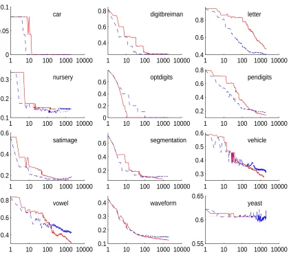
Figure 5: Training error curves: solid: AdaBoost.M2, dashed: GrPloss, dotted: BoostMA

differences in the group proportions, but also from differences in the resampling step and from the partition of a balanced data set into unbalanced training and test sets during cross-validation.

Performing a boosting algorithm is a time consuming procedure, so the speed of an algorithm is an important topic. Figure 5 indicates that the training error rate of GrPloss is decreasing faster than the training error rate of AdaBoost.M2. To be more precise, we look at the number of boosting rounds needed to achieve 90% of the total decrease of the training error rate. For 10 of the 12 data sets, AdaBoost.M2 needs more boosting rounds than GrPloss, so GrPloss seems to lead to a faster decrease in the training error rate (Table 4). Besides the number of boosting rounds, the time for the algorithm is also heavily influenced by the time needed to construct a base classifier. In our program, it took longer to construct a base classifier for AdaBoost.M2 because the minimization of the pseudo-loss which is required for AdaBoost.M2 is not as straightforward as the maximization of rt required for GrPloss and BoostMA. However, the time needed to construct a base classifier

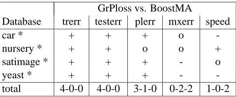
GrPloss vs. BoostMA

Database trerr testerr plerr mxerr speed

car * + + + o

-nursery * + + o o +

satimage * + + + - o

yeast * + + + -

-total 4-0-0 4-0-0 3-1-0 0-2-2 1-0-2

Table 5: Comparison of GrPloss with BoostMA for the unbalanced data sets: win-loss-table for the training error, test error, pseudo-loss error, maxlabel error and speed of the algorithm (+/o/-: win/draw/loss for GrPloss)

5. Conclusion

We proposed two new algorithms GrPloss and BoostMA for multiclass problems with weak base classifiers. The algorithms are designed to minimize the pseudo-loss error and the maxlabel error respectively. Both have the advantage that the base classifier minimizes the confidence-rated error instead of the pseudo-loss. This makes them easier to use with already existing base classifiers. Also the changes to AdaBoost.M1 are very small, so one can easily get the new algorithms by only slight adaption of the code of AdaBoost.M1. Although they are not designed to minimize the training error, they have comparable performance as AdaBoost.M2 in our experiments. As a second advantage, they converge faster than AdaBoost.M2. AdaBoost.M2 minimizes a bound on the training error. The other two algorithms have the disadvantage of minimizing bounds on performance measures which are not connected so strongly to the expected error. However the bounds on the performance measures of GrPloss and BoostMA are tighter than the bound on the training error of AdaBoost.M2, which seems to compensate for this disadvantage.

References

Erin L. Allwein, Robert E. Schapire, Yoram Singer. Reducing multiclass to binary: A unifying approach for margin classifiers. Machine Learning, 1:113–141, 2000.

Eric Bauer, Ron Kohavi. An empirical comparison of voting classification algorithms: bagging, boosting and variants. Machine Learning, 36:105–139, 1999.

Catherine Blake, Christopher J. Merz. UCI Repository of machine learning databases

[http://www.ics.uci.edu/ mlearn/MLRepository.html]. Irvine, CA: University of California, De-partment of Information and Computer Science, 1998

Thomas G. Dietterrich, Ghulum Bakiri. Solving multiclass learning problems via error-correcting output codes. Journal of Artificial Intelligence Research 2:263–286, 1995.

G¨unther Eibl, Karl–Peter Pfeiffer. How to make AdaBoost.M1 work for weak classifiers by chang-ing only one line of the code. Machine Learnchang-ing: Proceedchang-ings of the Thirteenth European Con-ference, 109–120, 2002.

Yoav Freund, Robert E. Schapire. Experiments with a new boosting algorithm. Machine Learning: Proceedings of the Thirteenth International Conference, 148–56, 1996.

Yoav Freund, Robert E. Schapire. A decision-theoretic generalization of online-learning and an application to boosting. Journal of Computer and System Sciences, 55(1):119–139, 1997.

Venkatesan Guruswami, Amit Sahai. Multiclass learning, boosting, and error-correcting codes. Proceedings of the Twelfth Annual Conference on Computational Learning Theory, 145–155, 1999.

Llew Mason, Peter L. Bartlett, Jonathan Baxter. Direct optimization of margins improves general-ization in combined classifiers. Proceedings of NIPS 98, 288–294, 1998.

Llew Mason, Peter L. Bartlett, Jonathan Baxter, Marcus Frean. Functional gradient techniques for combining hypotheses. Advances in Large Margin Classifiers, 221–246, 1999.

Ross Quinlan. Bagging, boosting, and C4.5. Proceedings of the Thirteenth National Conference on Artificial Intelligence, 725–730, 1996.

Gunnar R¨atsch, Bernhard Sch¨olkopf, Alex J. Smola, Sebastian Mika, Takashi Onoda, Klaus R. M¨uller. Robust ensemble learning. Advances in Large Margin Classifiers, 207–220, 2000a.

Gunnar R¨atsch, Takashi Onoda, Klaus R. M¨uller. Soft margins for AdaBoost. Machine Learning 42(3):287–320, 2000b.

Robert E. Schapire, Yoav Freund, Peter L. Bartlett, Wee Sun Lee. Boosting the margin: A new explanation for the effectiveness of voting methods. Annals of Statistics, 26(5):1651–1686, 1998.