Loopy Belief Propagation: Convergence and Effects of Message Errors
Alexander T. Ihler [email protected]
Donald Bren School of Information and Computer Science University of California, Irvine
Irvine, CA 92697 USA
John W. Fisher III [email protected]
Alan S. Willsky [email protected]
Massachusetts Institute of Technology Cambridge, MA 02139, USA
Editor: David Maxwell Chickering
Abstract
Belief propagation (BP) is an increasingly popular method of performing approximate inference on arbitrary graphical models. At times, even further approximations are required, whether due to quantization of the messages or model parameters, from other simplified message or model representations, or from stochastic approximation methods. The introduction of such errors into the BP message computations has the potential to affect the solution obtained adversely. We analyze the effect resulting from message approximation under two particular measures of error, and show bounds on the accumulation of errors in the system. This analysis leads to convergence conditions for traditional BP message passing, and both strict bounds and estimates of the resulting error in systems of approximate BP message passing.
Keywords: belief propagation, sum-product, convergence, approximate inference, quantization
1. Introduction
Graphical models and message-passing algorithms defined on graphs comprise a growing field of research. In particular, the belief propagation (or sum-product) algorithm has become a popular means of solving inference problems exactly or approximately. One part of its appeal lies in its optimality for tree-structured graphical models (models which contain no loops). However, its is also widely applied to graphical models with cycles. In these cases it may not converge, and if it does its solution is approximate; however in practice these approximations are often good. Recently, some additional justifications for loopy belief propagation have been developed, including a handful of convergence results for graphs with cycles (Weiss, 2000; Tatikonda and Jordan, 2002; Heskes, 2004).
2001). Additionally, simplification of complex graphical models through edge removal, quantiza-tion of the potential funcquantiza-tions, or other forms of distribuquantiza-tional approximaquantiza-tion may be considered in this framework. Finally, one may wish to approximate the messages and reduce their representation size for another reason—to decrease the communications required for distributed inference applica-tions. In distributed message passing, one may approximate the transmitted message to reduce its representational cost (Ihler et al., 2004a), or discard it entirely if it is deemed “sufficiently similar” to the previously sent version (Chen et al., 2004). Through such means one may significantly reduce the amount of communications required.
Given that message approximation may be desirable, we would like to know what effect the errors introduced have on our overall solution. In order to characterize the approximation effects in graphs with cycles, we analyze the deviation from the solution given by “exact” loopy belief propagation (not, as is typically considered, the deviation of loopy BP from the true marginal distri-butions). As a byproduct of this analysis, we also obtain some results on the convergence of loopy belief propagation.
We begin in Section 2 by briefly reviewing the relevant details of graphical models and be-lief propagation. Section 4 then examines the consequences of measuring a message error by its dynamic range. In particular, we explain the utility of this measure and its behavior with respect to the operations of belief propagation. This allows us to derive conditions for the convergence of traditional loopy belief propagation, and bounds on the distance between any pair of BP fixed points (Sections 5.1–5.2), and these results are easily extended to many approximate forms of BP (Section 5.3). If the errors introduced are independent, as is a typical assumption in, for example, quantization analysis (Gersho and Gray, 1991; Willsky, 1978), tighter estimates of the resulting error can be obtained (Section 5.5).
It is also instructive to examine other measures of message error, in particular ones which em-phasize more average-case (as opposed to pointwise or worst-case) differences. To this end, we consider a KL-divergence based measure in Section 6. While the analysis of the KL-divergence measure is considerably more difficult and does not lead to strict guarantees, it serves to give some intuition into the behavior of perturbed BP under an average-case difference measure.
2. Graphical Models
Graphical models (Lauritzen, 1996; Kschischang et al., 2001) provide a convenient means of rep-resenting conditional independence relations among large numbers of random variables. Specif-ically, each node s in an undirected graph is associated with a random variable xs, while the set of edges
E
is used to describe the conditional dependency structure of the variables throughgraph separation. If every path between two sets A and C passes through another set B [see Fig-ure 1(a)], the sets of variables xA={xs: s∈A}and xC={xs: s∈C}must be independent given the values of xB={xs : s∈B}. Thus, the distribution p(xA,xB,xC) can be written in the form
p(xB)p(xA|xB)p(xC|xB).
It can be shown that a distribution p(x)is consistent with (i.e., satisfies the conditional indepen-dence relations specified by) an undirected graph if it factors into a product of potential functions
u
u
u
t s
1
2
3
1 1
1 1 1 1
2
2
2 2
3 3
3 4
4
4
3 4
(a) (b) (c)
Figure 1: (a) Graphical models describe statistical dependency; here, the sets A and C are independent given B. (b) BP propagates information from t and its neighbors uiis to s by a simple message-passing procedure; this procedure is exact on a tree, but approximate in graphs with cycles. (c) For a graph with cycles, one may show an equivalence between n iterations of loopy BP and the depth-n computatiodepth-n tree [showdepth-n here for depth-n=3 and rooted at node1; example from Tatikonda and Jordan (2002)].
models with at most pairwise potential functions, so that the distribution factors according to
p(x) =
∏
(s,t)∈E
ψst(xs,xt)
∏
sψs(xs).
This is a typical assumption for belief propagation, and can be taken without incurring any real loss of generality since a graphical model with higher-order potential functions may always be converted to a graphical model with only pairwise potential functions through a process of variable augmenta-tion, though this may also increase the nodes’ state dimension undesirably; see, for example, Weiss (2000).
2.1 Belief Propagation
The goal of belief propagation (BP) (Pearl, 1988), also called the sum-product algorithm, is to compute the marginal distribution p(xt) at each node t. BP takes the form of a message-passing algorithm between nodes, expressed in terms of an update to the outgoing message at iteration i from each node t to each neighbor s in terms of the previous iteration’s incoming messages from t’s neighborsΓt [see Figure 1(b)],
mits(xs)∝
Z
ψts(xt,xs)ψt(xt)
∏
u∈Γt\smi−1ut (xt)dxt. (1)
Typically each message is normalized so as to integrate to unity (and we assume that such normal-ization is possible). For discrete-valued random variables, of course, the integral is replaced by a summation. At any iteration, one may calculate the belief at node t by
Mti(xt)∝ ψt(xt)
∏
u∈Γtmiut(xt). (2)
models by following the same local message passing rules at each node and ignoring the presence of cycles in the graph; this procedure is typically referred to as “loopy” BP.
For loopy BP, the sequence of messages defined by (1) is not guaranteed to converge to a fixed point after any number of iterations. Under relatively mild conditions, one may guarantee the ex-istence of fixed points (Yedidia et al., 2004). However, they may not be unique, nor are the results exact [the belief Mtidoes not converge to the true marginal p(xt)]. In practice however the procedure often arrives at a reasonable set of approximations to the correct marginal distributions.
2.2 Computation Trees
It is sometimes convenient to think of loopy BP in terms of its computation tree. Tatikonda and Jordan (2002) showed that the effect of n iterations of loopy BP at any particular node s is equivalent to exact inference on a tree-structured ‘unrolling” of the graph from s. A small graph, and its associated 4-level computation tree rooted at node1, are shown in Figure 1(c).
The computation tree with depth n consists of all length-n paths emanating from s in the original graph which do not immediately backtrack (though they may eventually repeat nodes).1 We draw the computation tree as consisting of a number of levels, corresponding to each node in the tree’s distance from the root, with the root node at level 0 and the leaf nodes at level n. Each level may contain multiple replicas of each node, and thus there are potentially many replicas of each node in the graph. The root node s has replicas of all neighborsΓsin the original graph as children, while all other nodes have replicas of all neighbors except their parent node as children.
Each edge in the computation tree corresponds to both an edge in the original graph and an iteration in the BP message-passing algorithm. Specifically, assume an equivalent initialization of both the loopy graph and computation tree—i.e., the initial messages m0ut in the loopy graph are taken as inputs to the leaf nodes. Then, the upward messages from level n to level n−1 match the messages m1ut in the first iteration of loopy BP, and more generally, a upward message miut on the computation tree which originates from a node u on level n−i+1 to its parent node t on level n−i is identical to the message from node u to node t in the ithiteration of loopy BP (out of n total iterations) on the original graph. Thus, the incoming messages to the root node (level 0) correspond to the messages in the nthiteration of loopy BP.
2.3 Message Approximations
Let us now consider the concept of approximate BP messages. We begin by assuming that the “true” messages mts(xs)are some fixed point of BP, so that mits=mits+1. We may ask what happens when these messages are perturbed by some (perhaps small) error function ets(xs). Although there are certainly other possibilities, the fact that BP messages are combined by taking their product makes it natural to consider multiplicative message deviations (or additive in the log-domain):
ˆ
mits(xs) =mts(xs)eits(xs).
To facilitate our analysis, we split the message update operation (1) into two parts. In the first, we focus on the message products
ˆ
Mtsi (xt)∝ ψt(xt)
∏
u∈Γt\sˆ
miut(xt) Mˆit(xt)∝ ψt(xt)
∏
u∈Γtˆ
miut(xt) (3)
where the proportionality constant is chosen to normalize ˆM. The second operation, then, is the message convolution
ˆ
mits+1(xs)∝
Z
ψts(xs,xt)Mˆtsi (xt)dxt (4)
where again ˆM is a normalized message or product of messages.
In this paper, we use the convention that lowercase quantities (mts,ets, . . .) refer to messages and message errors, while uppercase ones (Mts,Ets,Mt, . . .) refer to their products—at node t, the product of all incoming messages and the local potential is denoted Mt(xt), its approximation ˆMt(xt) =
Mt(xt)Et(xt), with similar definitions for Mts, ˆMts, and Ets.
3. Overview of Results
To orient the reader, we lay out the order and general results which are obtained in this paper. We begin in Section 4 by examining a dynamic range measure d(e)of the variability of a message error e(x) (or more generally of any function) and show how this measure behaves with respect to the BP equations (1) and (2). Specifically, we show in Section 4.2 that the measure log d(e)is sub-additive with respect to the product operation (3), and contractive with respect to the convolution operation (4).
Applying these results to traditional belief propagation results in a new sufficient condition for BP convergence (Section 5.1), specifically
max s,t
∑
u∈Γt\s
d(ψut)2−1
d(ψut)2+1
<1; (5)
and this condition may be further improved in many cases. The condition (5) can be shown to be slightly stronger than the sufficient condition given in Tatikonda and Jordan (2002), and empirically appears to be stronger than that of Heskes (2004). In experiments, the condition appears to be tight (exactly predicting uniqueness or non-uniqueness of fixed points) for at least some problems, such as binary–valued random variables with attractive potentials. More importantly, however, the method in which it is derived allows us to generalize to many other situations:
1. Using the same methodology, we may demonstrate that any two BP fixed points must be within a ball of a calculable diameter; the condition (5) is equivalent to this diameter being zero (Section 5.2).
2. Both the diameter of the bounding ball and the convergence criterion (5) are easily improved for graphical models with irregular geometry or potential strengths, leading to better condi-tions on graphs which are more “tree-like” (Section 5.3).
3. The same analysis may also be applied to the case of quantized or otherwise approximated messages and models (potential functions), yielding bounds on the resulting error (Section 5.4).
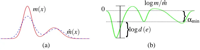
m(x)
ˆ
m(x)
}
}
0
log d(e)
αmin
log m/mˆ
(a) (b)
Figure 2: (a) A message m(x) and an example approximation mˆ(x); (b) their log-ratio log m(x)/mˆ(x), and the error measure log d(e).
Finally, in Section 6 we perform the same analysis for a less strict measure of message error [i.e., disagreement between a message m(x)and its approximation ˆm(x)], namely the Kullback-Leibler divergence. This analysis shows that, while failing to provide strict bounds in several key ways, one is still able to obtain some intuition into the behavior of approximate message passing under an average-case difference measure.
In the next few sections, we first describe the dynamic range measure and discuss some of its salient properties (Section 4). We then apply these properties to analyze the behavior of loopy belief propagation (Section 5). Almost all proofs are given in an in-line fashion, as they frequently serve to give intuition into the method and meaning of each result.
4. Dynamic Range Measure
In order to discuss the effects and propagation of errors, we first require a measure of the difference between two messages. In this section, we examine the following measure on ets(xs): let d(ets) denote the function’s dynamic range,2specifically
d(ets) =sup a,b
p
ets(a)/ets(b). (6)
Then, we have that mts≡mˆts(i.e., the pointwise equality condition mts(x) =mˆts(x)∀x) if and only if log d(ets) =0. Figure 2 shows an example of m(x)and ˆm(x)along with their associated error e(x).
4.1 Motivation
We begin with a brief motivation for this choice of error measure. It has a number of desirable features; for example, it is directly related to the pointwise log error between the two distributions.
Lemma 1. The dynamic range measure (6) may be equivalently defined by log d(ets) =infα sup
x
|logαmts(x)−log ˆmts(x)|=infα sup x
|logα−log ets(x)|.
Proof. The minimum is given by logα=1
2(supalog ets(a) +infblog ets(b)), and thus the right-hand side is equal to 12(supalog ets(a)−infblog ets(b)), or12(supa,blog ets(a)/ets(b)), which by definition is log d(ets).
The scalarαserves the purpose of “zero-centering” the function log ets(x)and making the mea-sure invariant to simple rescaling. This invariance reflects the fact that the scale factor for BP messages is essentially arbitrary, defining a class of equivalent messages. Although the scale factor cannot be completely ignored, it takes on the role of a nuisance parameter. The inclusion ofαin the definition of Lemma 1 acts to select particular elements of the equivalence classes (with respect to rescaling) from which to measure distance—specifically, choosing the closest such messages in a log-error sense. The log-error, dynamic range, and the minimizingαare depicted in Figure 2.
Lemma 1 allows the dynamic range measure to be related directly to an approximation error in the log-domain when both messages are normalized to integrate to unity, using the following theorem:
Theorem 2. The dynamic range measure can be used to bound the log-approximation error:
|log mts(x)−log ˆmts(x)| ≤2 log d(ets) ∀x.
Proof. We first consider the magnitude of logα:
∀x,
logαmts(x) ˆ mts(x)
≤log d(ets)
⇒ 1
d(ets)
≤αmts(x) ˆ mts(x)
≤d(ets)
⇒
Z
ˆ mts(x)dx
1 d(ets)
≤α
Z
mts(x)dx≤
Z
ˆ
mts(x)dxd(ets)
and since the messages are normalized,|logα| ≤log d(ets). Then by the triangle inequality,
|log mts(x)−log ˆmts(x)| ≤ |logαmts(x)−log ˆmts(x)|+|logα| ≤2 log d(ets).
In this light, our analysis of message approximation (Section 5.4) may be equivalently regarded as a statement about the required quantization level for an accurate implementation of loopy belief propagation. Interestingly, it may also be related to a floating-point precision on mts(x).
Lemma 3. Let ˆmts(x)be an F-bit mantissa floating-point approximation to mts(x). Then, log d(ets)≤ 2−F+
O
(2−2F).Proof. For an F-bit mantissa, we have|mts(x)−mˆts(x)|<2−F·2blog2mts(x)c≤2−F·mts(x). Then, using the Taylor expansion of log1+ (mˆ
m−1)
≈(mˆ
m−1)we have that
log d(ets)≤sup x
logmˆ(x) m(x)
≤sup x ˆ
m(x)−m(x)
m(x) +
O
sup x
ˆ
m(x)−m(x)
m(x)
2!
≤2−F+
O
2−2F.
Lemma 4. The KL-divergence satisfies the inequality D(mtskmˆts)≤2 log d(ets)
Proof. By Theorem 2, we have
D(mtskmˆts) =
Z
mts(x)log
mts(x) ˆ mts(x)
dx≤
Z
mts(x) (2 log d(ets))dx=2 log d(ets).
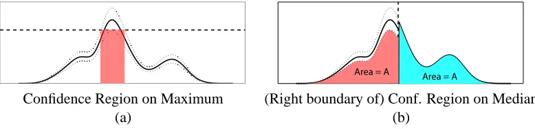
Finally, a bound on the dynamic range or the absolute log-error can also be used to develop confidence intervals for the maximum and median of the distribution.
Lemma 5. Let ˆm(x)be an approximation of m(x)with log d(mˆ/m)≤ε, so that
ˆ
m+(x) =exp(2ε)mˆ(x) mˆ−(x) =exp(−2ε)mˆ(x)
are upper and lower pointwise bounds on m(x), respectively. Then we have a confidence region on the maximum of m(x)given by
arg max
x m(x)∈ {x : ˆm
+(x)≥max y mˆ
−(y)}
and an upper bound µ on the median of m(x), i.e.,
Z µ
−∞m(x)≥
Z ∞
µ
m(x) where
Z µ
−∞mˆ
−(x) =Z ∞ µ
ˆ m+(x)
with a similar lower bound.
Proof. The definitions of ˆm+and ˆm− follow from Theorem 2. Given these bounds, the maximum value of m(x)must be larger than the maximum value of ˆm−(x), and this is only possible at locations x for which ˆm+(x)is also greater than the maximum of ˆm−. Similarly, the left integral of m(x)(−∞ to µ) must be larger than the integral of ˆm−(x), while the right integral (µ to∞) must be smaller than for ˆm+(x). Thus the median of m(x)must be less than µ.
These bounds and confidence intervals are illustrated in Figure 3: given the approximate mes-sage ˆm (solid black), a bound on the error yields ˆm+(x) and ˆm−(x) (dotted lines), which yield confidence regions on the maximum and median values of m(x).
4.2 Additivity and Error Contraction
We now turn to the properties of our dynamic range measure with respect to the operations of belief propagation. First, we consider the error resulting from taking the product (3) of a number of incoming approximate messages.
Theorem 6. The log of the dynamic range measure is sub-additive:
log d Etsi≤
∑
u∈Γt\slog d eiut log d Eti≤
∑
u∈ΓtArea = A
Area = A
Confidence Region on Maximum (Right boundary of) Conf. Region on Median
(a) (b)
Figure 3: Using the error measure (6) to find confidence regions on maximum and median lo-cations of a distribution. The distribution estimate ˆm(x) is shown in solid black, with |log m(x)/mˆ(x)| ≤ 1
4 bounds shown as dotted lines. Then, the maximum value of m(x) must lie above the shaded region, and the median value is less than the dashed vertical line; a similar computation gives a lower bound.
Proof. We show the left-hand sub-additivity statement; the right follows from a similar argument. By definition, we have
log d Etsi=log d Mˆtsi /Mtsi =1
2log supa,b
∏
eiut(a)/
∏
eiut(b).Increasing the number of degrees of freedom gives
≤1
2log
∏
ausup,bueiut(au)/eiut(bu) =
∑
log d eiut(x)
.
Theorem 6 allows us to bound the error resulting from a combination of the incoming approx-imations from two different neighbors of the node t. It is also important that log d(e) satisfy the triangle inequality, so that the application of two successive approximations results in an error which is bounded by the sum of their respective errors.
Theorem 7. The log of the dynamic range measure satisfies the triangle inequality: log d(e1e2)≤log d(e1) +log d(e2).
Proof. This follows from the same argument as Theorem 6.
We may also derive a minimum rate of contraction occurring with the convolution operation (4). We characterize the strength of the potentialψts by extending the definition of the dynamic range measure:
d(ψts)2= sup a,b,c,d
ψts(a,b)
ψts(c,d)
. (7)
When this quantity is finite, it represents a minimum rate of mixing for the potential, and thus causes a contraction on the error. This fact is exhibited in the following theorem.
Theorem 8. When d(ψts)is finite, the dynamic range measure satisfies a rate of contraction:
d eits+1≤d(ψts) 2d Ei
ts
+1
d(ψts)2+d Etsi
logd(ψ)2d(E)+1
d(ψ)2+d(E)
log d(E)
log d(ψ)2
log
d
(
e
)
→
log d(E) →
Figure 4: Three bounds on the error output d(e)as a function of the error on the product of incom-ing messages d(E).
Proof. See Appendix A.
Two limits are of interest. First, if we examine the limit as the potential strength d(ψ)grows, we see that the error cannot increase due to convolution with the pairwise potentialψ. Similarly, if the potential strength is finite, the outgoing error cannot be arbitrarily large (independent of the size of the incoming error).
Corollary 9. The outgoing message error d(ets)is bounded by
d eits+1
≤d Etsi
d eits+1
≤d(ψts)2.
Proof. Let d(ψts)or d Etsi
tend to infinity in Theorem 8.
The contractive bound (8) is shown in Figure 4, along with the two simpler bounds of Corol-lary 9, shown as straight lines. Moreover, we may evaluate the asymptotic behavior by considering the derivative
∂
∂d(E)
d(ψ)2d(E) +1 d(E) +d(ψ)2
d(E)→1
=d(ψ) 2
−1
d(ψ)2+1=tanh(log d(ψ)).
The limits of this bound are quite intuitive: for log d(ψ) =0 (independence of xt and xs), this deriva-tive is zero; increasing the error in incoming messages miut has no effect on the error in mits+1. For
d(ψ)→∞, the derivative approaches unity, indicating that for very large d(ψ)(strong potentials) the propagated error can be nearly unchanged.
5. Applying Dynamic Range to Graphs with Cycles
In this section, we apply the framework developed in Section 4, along with the computation tree formalism of Tatikonda and Jordan (2002), to derive results on the behavior of traditional belief propagation (in which messages and potentials are represented exactly). We then use the same methodology to analyze the behavior of loopy BP for quantized or otherwise approximated mes-sages and potential functions.
5.1 Convergence of Loopy Belief Propagation
The work of Tatikonda and Jordan (2002) showed that the convergence and fixed points of loopy BP may be considered in terms of a Gibbs measure on the graph’s computation tree. In particular, this led to the result that loopy BP is guaranteed to converge if the graph satisfies Dobrushin’s condition (Georgii, 1988). Dobrushin’s condition is a global measure, and difficult to verify; given in Tatikonda and Jordan (2002) is the easier to check sufficient condition (often called Simon’s condition),
Theorem 10 (Simon’s condition). Loopy belief propagation is guaranteed to converge if max
t
∑
u∈Γtlog d(ψut)<1. (9)
where d(ψ)is defined as in (7).
Proof. See Tatikonda and Jordan (2002).
Using the previous section’s analysis, we obtain the following, stronger condition, and (after the proof) show analytically how the two are related.
Theorem 11 (BP convergence). Loopy belief propagation is guaranteed to converge if
max (s,t)∈E
∑
u∈Γt\s
d(ψut)2−1
d(ψut)2+1
<1 (10)
Proof. By induction. Let the “true” messages mts be any fixed point of BP, and consider the in-coming error observed by a node t at level n−1 of the computation tree (corresponding to the first iteration of BP), and having parent node s. Suppose that the total incoming error log d Ets1 is bounded above by some constant logε1 for all(t,s)∈
E
. Note that this is trivially true (for anyn) for the constant logε1=maxt∑u∈Γtlog d(ψut) 2
, since the error on any message mut is bounded above by d(ψut)2.
Now, assume that log d Euti ≤logεi for all(u,t)∈
E
. Theorem 8 bounds the maximum log-error log d Etsi+1
at any replica of node t with parent s, where s is on level n−i of the tree (which corresponds to the ithiteration of loopy BP) by
log d Etsi+1≤gts(logεi) =Gts(εi) =
∑
u∈Γt\slogd(ψut) 2εi+1
d(ψut)2+εi
. (11)
Defining z=logε, we may equivalently show gts(z)<z for all z>0. This can be guaranteed by the conditions gts(0) =0, g0ts(0)<1, and g00ts(z)≤0 for each t,s. The first is easy to verify, as is the last (term by term) using the identity g00ts(z) =ε2G00
ts(ε) +εG0ts(ε); the second (gts0 (0)<1) can be rewritten to give the convergence condition (10).
We may relate Theorem 11 to Simon’s condition by expanding the set Γt\s to the larger set
Γt, and observing that log x≥ x
2−1
x2+1 for all x≥1 with equality as x→1. Doing so, we see that
Simon’s condition is sufficient to guarantee Theorem 11, but that Theorem 11 may be true (implying convergence) when Simon’s condition is not satisfied. The improvement over Simon’s condition becomes negligible for highly-connected systems with weak potentials, but can be significant for graphs with low connectivity. For example, if the graph consists of a single loop then each node t has at most two neighbors. In this case, the contraction (11) tells us that the outgoing message in either direction is always as close or closer to the BP fixed point than the incoming message. Thus we easily obtain the result of Weiss (2000), that (for finite-strength potentials) BP always converges to a unique fixed point on graphs containing a single loop. Simon’s condition, on the other hand, is too loose to demonstrate this fact. The form of the condition in Theorem 11 is also similar to a result shown for binary spin models; see Georgii (1988) for details.
However, both Theorem 10 and Theorem 11 depend only on the pairwise potentialsψst(xs,xt), and not on the single-node potentials ψs(xs), ψt(xt). As noted by Heskes (Heskes, 2004), this leaves a degree of freedom to which the single-node potentials may be chosen so as to minimize the (apparent) strength of the pairwise potentials. Thus, (9) can be improved slightly by writing
max t
∑
u∈Γt min
ψu,ψt log d
ψ
ut
ψuψt
<1 (12)
and similarly for (10) by writing
max (s,t)∈E
∑
u∈Γt\s min
ψu,ψt
d
ψ
ut
ψuψt
2
−1
d
ψ
ut
ψuψt
2
+1
<1. (13)
To evaluate this quantity, one may also observe that
min
ψu,ψt
d
ψ
ut
ψuψt
4
= sup a,b,c,d
ψts(a,b)
ψts(a,d)
ψts(c,d)
ψts(c,b)
.
In general we shall ignore this subtlety and simply write our results in terms of d(ψ), as given in (9) and (10). For binary random variables, it is easy to see that the minimum–strengthψuthas the form
ψut=
η
1−η
1−η η
,
and that when the potentials are of this form (such as in the examples of this section) the two conditions are completely equivalent.
5.2 Distance of Multiple Fixed Points
Theorem 11 may be extended to provide not only a sufficient condition for a unique BP fixed point, but an upper bound on distance between the beliefs generated by successive BP updates and any BP fixed point. Specifically, the proof of Theorem 11 relied on demonstrating a bound logεi on the distance from some arbitrarily chosen fixed point{Mt} at iteration i. When this bound decreases to zero, we may conclude that only one fixed point exists. However, even should it decrease only to some positive constant, it still provides information about the distance between any iteration’s belief and the fixed point. Moreover, applying this bound to another, different fixed point{M˜t}tells us that all fixed points of loopy BP must lie within a sphere of a given diameter [as measured by log d Mt/M˜t
]. These statements are made precise in the following two theorems:
Theorem 12 (BP distance bound). Let{Mt} be any fixed point of loopy BP. Then, after n>1
iterations of loopy BP resulting in beliefs{Mˆn
t}, for any node t and for all x
log d Mt/Mˆtn
≤
∑
u∈Γt
logd(ψut)
2εn−1+1
d(ψut)2+εn−1
whereεiis given byε1=maxs,td(ψst)2and
logεi+1= max (s,t)∈E
∑
u∈Γt\s
logd(ψut) 2εi+1
d(ψut)2+εi
.
Proof. The result follows directly from the proof of Theorem 11.
We may thus infer a distance bound between any two BP fixed points:
Theorem 13 (Fixed-point distance bound). Let{Mt},{M˜t}be the beliefs of any two fixed points
of loopy BP. Then, for any node t and for all x
|log Mt(x)/M˜t(x)| ≤2 log d Mt/M˜t
≤2
∑
u∈Γtlogd(ψut) 2ε
+1 d(ψut)2+ε
(14)
whereεis the largest value satisfying
logε= max
(s,t)∈EGts(ε) =(maxs,t)∈E
∑
u∈Γt\s
logd(ψut) 2ε
+1 d(ψut)2+ε
. (15)
Proof. The inequality|log Mt(x)/M˜t(x)| ≤2 log d Mt/M˜t
follows from Theorem 2. The rest fol-lows from Theorem 12—taking the “approximate” messages to be any other fixed point of loopy BP, we see that the error cannot decrease over any number of iterations. However, by the same argument given in Theorem 11, g00ts(z)<0, and for z sufficiently large, gts(z)<z. Thus (15) has at most one solution greater than unity, andεi+1<εifor all i withεi→εas i→∞. Letting the number of iterations i→∞, we see that the message “errors” log d Mts/M˜ts
Thus, if the value of logεis small (the sufficient condition of Theorem 11 is nearly satisfied) then although we cannot guarantee convergence to a unique fixed point, we can still make a strong statement: that the set of fixed points are all mutually close (in a log-error sense), and reside within a ball of diameter described by (14). Moreover, even though it is possible that loopy BP does not con-verge, and thus even after infinite time the messages may not correspond to any fixed point of the BP equations, we are guaranteed by Theorem 12 that the resulting belief estimates will asymptotically approach the same bounding ball [achieving distance at most (14) from all fixed points].
5.3 Path-Counting
If we are willing to put a bit more effort into our bound-computation, we may be able to improve it further, since the bounds derived using computation trees are very much “worst-case” bounds. In particular, the proof of Theorem 11 assumes that, as a message error propagates through the graph, repeated convolution with only the strongest set of potentials is possible. But often even if the worst potentials are quite strong, every cycle which contains them may also contain several weaker potentials. Using an iterative algorithm much like belief propagation itself, we may obtain a more globally aware estimate of how errors can propagate through the graph.
Theorem 14 (Non-uniform distance bound). Let{Mt}be any fixed point belief of loopy BP. Then,
after n≥1 iterations of loopy BP resulting in beliefs{Mˆtn}, for any node t and for all x
|log Mt(x)/Mˆt(x)| ≤2 log d Mt/Mˆtn
≤2
∑
u∈Γtlogυnut
whereυiut is defined by the iteration
logυtsi+1=logd(ψts) 2εi
ts+1
d(ψts)2+εtsi
logεits=
∑
u∈Γt\slogυiut (16)
with initial conditionυ1ut=d(ψut)2.
Proof. Again we consider the error log d Etsi
incoming to node t with parent s, where t is at level n−i+1 of the computation tree. Using the same arguments as Theorem 11 it is easy to show by induction that the error products log d Etsi are bounded above byεits, and the individual message errors log d etsi are bounded above byυtsi , and . Then, by additivity we obtain the stated bound on d(Etn)at the root node.
The iteration defined in Theorem 14 can also be interpreted as a (scalar) message-passing proce-dure, or may be performed offline. As before, if this procedure results in logεts→0 for all(t,s)∈
E
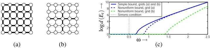
we are guaranteed that there is a unique fixed point for loopy BP; if not, we again obtain a bound on the distance between any two fixed-point beliefs. When the graph is perfectly symmetric (every node has identical neighbors and potential strengths), this yields the same bound as Theorem 12; however, if the potential strengths are inhomogeneous Theorem 14 provides a strictly better bound on loopy BP convergence and errors.This situation is illustrated in Figure 5—we specify two different graphical models defined on a 5×5 grid in terms of their potential strengths log d(ψ)2, and compute bounds on the dynamic range d Mt/M˜t
0 0.5 1 1.5 2 2.5 0
2 4 6 8 10
Simple bound, grids (a) and (b) Nonuniform bound, grid (a) Nonuniform bound, grid (b) Simons condition
lo
g
d
(
Et
)
→
ω→
(a) (b) (c)
Figure 5: (a-b) Two small (5×5) grids. In (a), the potentialsψare all of equal strength (log d(ψ)2=
ω), while in (b) several potentials (thin lines) are weaker (log d(ψ)2=.5ω). The methods described may be used to compute bounds (c) on the distance d(Et) between any two fixed point beliefs as a function of potential strengthω.
does not completely specify the graphical model, it is sufficient for all the bounds considered here.) One grid (a) has equal-strength potentials log d(ψ)2=ω, while the other has many weaker potentials (ω/2). The worst-case bounds are the same (since both have a node with four strong neighbors), shown as the solid curve in (c). However, the dashed curves show the estimate of (16), which improves only slightly for the strongly coupled graph (a) but considerably for the weaker graph (b). All three bounds give considerably more information than Simon’s condition (dotted vertical line).
Having shown how our bound may be improved for irregular graph geometry, we may now com-pare our bounds to two other known uniqueness conditions (Tatikonda and Jordan, 2002; Heskes, 2004). Simon’s condition can be related analytically, as described in Section 5.1. On the other hand, the recent work of Heskes (2004) takes a very different approach to uniqueness based on analysis of the minima of the Bethe free energy, which directly correspond to stable fixed points of BP (Yedidia et al., 2004). This leads to an alternate sufficient condition for uniqueness. As observed in Heskes (2004) it is unclear whether a unique fixed point necessarily implies convergence of loopy BP. In contrast, our approach gives a sufficient condition for the convergence of BP to a unique solution, which implies uniqueness of the fixed point.
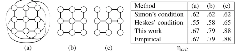
Showing an analytic relation between all three approaches does not appear straightforward; to give some intuition, we show the three example binary graphs compared in Heskes (2004), whose structures are shown in Figure 6(a-c) and whose potentials are parameterized by a scalar η> .5, namely
ψ=
η
1−η
1−η η
(17)
(so that d(ψ)2= 1−ηη). The trivial solution Mt = [.5;.5]is always a fixed point, but may not be stable; the preciseηcrit at which this fixed point becomes unstable (implying the existence of other, stable fixed points) can be found empirically for each case (Heskes, 2004); the same values may also be found algebraically by imposing symmetry requirements on the messages (Yedidia et al., 2004). This value may then be compared to the uniqueness bounds of Tatikonda and Jordan (2002), the bound of Heskes (2004), and this work; these are shown in Figure 6.
Method (a) (b) (c) Simon’s condition .62 .62 .62 Heskes’ condition .55 .58 .65
This work .67 .79 .88
Empirical .67 .79 .88
(a) (b) (c) ηcrit
Figure 6: Comparison of various uniqueness bounds: for binary potentials parameterized byη, we find the predictedηcritat which loopy BP can no longer be guaranteed to be unique. For these simple problems, theηcrit at which the trivial (correct) solution becomes unstable may be found empirically. Examples and empirical values ofηcritfrom Heskes (2004).
(2004), though without analytic comparison it is unclear whether this is always the case. In fact, for these simple binary examples, our bound appears to be tight.
However, our method also allows us to make statements about the results of loopy BP after finite numbers of iterations, up to some finite degree of numerical precision in the final results. For example, we may also find the value ofηbelow which BP will attain a particular precision, say log d Mt/Mˆtn
<10−3in at least n=100 iterations [obtaining the values{.66, .77, .85}for the grids in Figure 6(a), (b), and (c), respectively].
5.4 Introducing Intentional Message Errors and Censoring
As discussed in the introduction, we may wish to introduce or allow additional errors in our mes-sages at each stage, in order to improve the computational or communication efficiency of the algo-rithm. This may be the result of an actual distortion imposed on the message (perhaps to decrease its complexity, for example quantization), or the result of censoring the message update (reusing the message from the previous iteration) when the two are sufficiently similar. Errors may also arise from quantization or other approximation of the potential functions. Such additional errors may be easily incorporated into our framework.
Theorem 15. If at every iteration of loopy BP, each message is further approximated in such a way as to guarantee that the additional distortion has maximum dynamic range at mostδ, then for any fixed point beliefs{Mt}, after n≥1 iterations of loopy BP resulting in beliefs{Mˆnt}we have
log d Mt/Mˆtn
≤
∑
u∈Γt logυnut
whereυiut is defined by the iteration
logυtsi+1=logd(ψts) 2εi
ts+1
d(ψts)2+εtsi
+logδ logεits=
∑
u∈Γt\slogυiut
with initial conditionυ1ut=δd(ψut)2.
As with Theorem 14, a simpler bound can also be derived (similar to Theorem 12). Either gives a bound on the maximum total distortion from any true fixed point which will be incurred by quantized or censored belief propagation. Note that (except on tree-structured graphs) this does not bound the error from the true marginal distributions, only from the loopy BP fixed points.
It is also possible to interpret the additional error as arising from an approximation to the correct single-node and pairwise potentialsψt,ψts.
Theorem 16. Suppose that{Mt}are a fixed point of loopy BP on a graph defined by potentialsψts
andψt, and let{Mˆtn}be the beliefs of n iterations of loopy BP performed on a graph with potentials ˆ
ψtsand ˆψt, where d(ψˆts/ψts)≤δ1and d(ψˆt/ψt)≤δ2. Then, log d Mt/Mˆtn
≤
∑
u∈Γt
logυnut+logδ2
whereυiut is defined by the iteration
logυits+1=logd(ψts) 2εi
ts+1
d(ψts)2+εits
+logδ1 logεits=logδ2+
∑
u∈Γt\slogυiut
with initial conditionυ1ut=δ1d(ψut)2.
Proof. We first extend the contraction result given in Appendix A by applying the inequality
Rψ
(xt,a)ψψˆ((xtxt,,aa))M(xt)E(xt)dxt
Rψ
(xt,b)ψψˆ((xtxt,,bb))M(xt)E(xt)dxt ≤
Rψ
(xt,a)M(xt)E(xt)dxt
Rψ
(xt,b)M(xt)E(xt)dxt
·d(ψˆ/ψ)2.
Then, proceeding similarly to Theorem 15 yields the definition ofυits, and including the additional errors logδ2in each message product (resulting from the product with ˆψt rather thanψt) gives the definition ofεtsi .
Incorrect models ˆψmay arise when the exact graph potentials have been estimated or quantized; Theorem 16 gives us the means to interpret the (worst-case) overall effects of using an approximate model. As an example, let us again consider the model depicted in Figure 6(b). Suppose that we are given quantized versions of the pairwise potentials, ˆψ, specified by the value (rounded to two decimal places) η=.65. Then, the true potentialψ hasη∈.65±.005, and thus is within
δ1 ≈1.022= ((..34535)()(.655.65)) of the known approximation ˆψ. Applying the recursion of Theorem 16 allows us to conclude that the solution obtained using the approximate model ˆψand true modelψ are within log d(e)≤.36, or alternatively that the beliefs found using the approximate model are correct to within a multiplicative factor of about 1.43. The same ˆψ, withηassumed correct to three decimal places, gives a bound log d(e)≤.04, or multiplicative factor of 1.04.
5.5 Stochastic Analysis
Proposition 17. Suppose that the errors log ets are random and uncorrelated, so that at each
iter-ation i, for s6=u and any x, Elog eist(x)·log eiut(x)
=0, and that at each iteration of loopy BP, the additional error (in the log domain) imposed on each message is uncorrelated with variance at most(logδ)2. Then,
E
h
log d Eti2
i
≤
∑
u∈Γt
σi ut
2
(18)
whereσ1ts=log d(ψts)2and
σi+1 ts
2
= logd(ψts) 2λi
ts+1
d(ψts)2+λits
!2
+ (logδ)2 logλits2=
∑
u∈Γt\sσi ut
2
.
Proof. Let us define the (nuisance) scale factorαits=arg minαsupx|logαeits(x)|for each error etsi , and letζits(x) =logαtsi eits(x). Now, we model the error function ζtsi (x) (for each x) as a random variable with mean zero, and bound the standard deviation ofζits(x)byσtsi at each iteration i; under the assumption that the errors in any two incoming messages are uncorrelated, we may assert addi-tivity of their variances. Thus the variance of∑Γt\sζiut(x)is bounded by(logλtsi )2. The contraction of Theorem 8 is a non-linear relationship; we estimate its effect on the error variance using a sim-ple sigma-point quadrature (“unscented”) approximation (Julier and Uhlmann, 1996), in which the standard deviationσits+1is estimated by applying Theorem 8’s nonlinear contraction to the standard deviation of the error on the incoming product (logλits).
The assumption of uncorrelated errors is clearly questionable, since propagation around loops may couple the incoming message errors. However, similar assumptions have yielded useful analy-sis of quantization effects in assessing the behavior and stability of digital filters (Willsky, 1978). It is often the case that empirically, such systems behave similarly to the predictions made by assum-ing uncorrelated errors. Indeed, we shall see that in our simulations, the assumption of uncorrelated errors provides a good estimate of performance.
Given the bound (18) on the variance of log d(E), we may apply a Chebyshev-like argument to provide probabilistic guarantees on the magnitude of errors log d(E) observed in practice. In our experiments (Section 5.6), the 2σdistance was almost always larger than the observed error. The probabilistic bound derived using (18) is typically much smaller than the bound of Theorem 15 due to the strictly sub-additive relationship between the standard deviations. However, the underlying assumption of uncorrelated errors makes the estimate obtained using (18) unsuitable for deriving strict convergence guarantees.
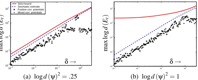
5.6 Experiments
10−3 10−2 10−1 100 10−3
10−2 10−1 100 101
Strict bound Stochastic estimate Positive corr. potentials Mixed corr. potentials
δ→
ma
x
lo
g
d
(
Et
)
10−3
10−2
10−1
100 10−3
10−2 10−1 100 101
δ→
ma
x
lo
g
d
(
Et
)
(a) log d(ψ)2=.25 (b) log d(ψ)2=1
Figure 7: Maximum belief errors incurred as a function of the quantization error. The scatterplot indicates the maximum error measured in the graph for each of 200 Monte Carlo runs; this is strictly bounded above by Theorem 15, solid, and bounded with high probability (assuming uncorrelated errors) by Proposition 17, dashed.
.
Also shown are two performance estimators—the bound on belief error developed in Sec-tion 5.4, and the 2σ estimate computed assuming uncorrelated message errors as in Section 5.5. As can be seen, the stochastic estimate is a much tighter, more accurate assessment of error, but it does not possess the same strong theoretical guarantees. Since [as observed for digital filtering ap-plications (Willsky, 1978)] the errors introduced by quantization are typically close to independent, the assumptions underlying the stochastic estimate are reasonable, and empirically we observe that the estimate and actual errors behave similarly.
6. KL-Divergence Measures
Although the dynamic range measure introduced in Section 4 leads to a number of strong guarantees, its performance criterion may be unnecessarily (and undesirably) strict. Specifically, it provides a pointwise guarantee, that m and ˆm are close for every possible state x. For continuous-valued states, this is an extremely difficult criterion to meet—for instance, it requires that the messages’ tails match almost exactly. In contrast, typical measures of the difference between two distributions operate by an average (mean squared error or mean absolute error) or weighted average (Kullback-Leibler divergence) evaluation. To address this, let us consider applying a measure such as the Kullback-Leibler (KL) divergence,
D(pkpˆ) =
Z
p(x)logp(x) ˆ p(x)dx.
viewpoint, since a strong disagreement between parts of the graph is unlikely we will be able to relax our error measure in the message tails.
Unfortunately, many of the properties which we relied on for analysis of the dynamic range measure do not strictly hold for a KL-divergence measure of error, resulting in an approximation, rather than a bound, on performance. In Appendix B, we give a detailed analysis of each property, showing the ways in which each aspect can break down and discussing the reasonability of simple approximations. In this section, we apply these approximations to develop a KL-divergence based estimate of error.
6.1 Local Observations and Parameterization
To make this notion concrete, let us consider a graphical model in which the single-node poten-tial functions are specified in terms of a set of observation variables y={yt}; in this section we will examine the average (expected) behavior of BP over multiple realizations of the observation variables y. We further assume that both the prior p(x) and likelihood p(y|x) exhibit conditional independence structure, expressed as a graphical model. Specifically, we assume throughout this section that the observation likelihood factors as
p(y|x) =
∏
tp(yt|xt), (19)
in other words, that each observation variable yt is local to (conditionally independent given) one of the xt. As for the prior model p(x), for the moment we confine our attention to tree-structured distributions, for which one may write (Wainwright et al., 2003)
p(x) =
∏
(s,t)∈E
p(xs,xt)
p(xs)p(xt)
∏
sp(xs). (20)
The expressions (19)-(20) give rise to a convenient parameterization of the joint distribution, ex-pressed as
p(x,y)∝
∏
(s,t)∈E
ψst(xs,xt)
∏
sψx
s(xs)ψys(xs) (21)
where
ψst(xs,xt) =
p(xs,xt)
p(xs)p(xt)
and ψxs(xs) =p(xs) , ψys(xs) =p(ys|xs). (22)
Our goal is to compute the posterior marginal distributions p(xs|y) at each node s; for the tree-structured distribution (21) this can be performed exactly and efficiently by BP. As discussed in the previous section, we treat the{yt}as random variables; thus almost all quantities in this graph are themselves random variables (as they are dependent on the yt), so that the single node observation potentialsψys(xs), messages mst(xt), etc. are random functions of their argument xs. The potentials due to the prior (ψstandψxs), however, are not random variables as they do not depend on any of the observations yt.
normalization of the messages mts, so that
R
p(xs)mts(xs) =1 (as opposed to
R
mts(xs) =1 as as-sumed previously); we again assume this prior-weighted normalization is always possible (this is trivially the case for discrete-valued states x). Then, for a tree-structured graph, the prior-weight normalized fixed-point message from t to s is precisely
mts(xs) =p(yts|xs)/p(yts) (23)
and the products of incoming messages to t, as defined in Section 2.3, are equal to
Mts(xt) =p(xt|yts) Mt(xt) =p(xt|y).
We may now apply a posterior-weighted log-error measure, defined by
D
(mutkmˆut) =Z
p(xt|y)log
mut(xt) ˆ mut(xt)
dxt; (24)
and may relate (24) to the Kullback-Leibler divergence.
Lemma 18. On a tree-structured graph, the error measure
D
(Mt,Mˆt) is equivalent to the KL-divergence of the true and estimated posterior distributions at node t:D
(MtkMˆt) =D(p(xt|y)kpˆ(xt|y)).Proof. This follows directly from the definitions of
D
, and the fact that on a tree, the unique fixed point has beliefs Mt(xt) =p(xt|y).Again, the error
D
(mutkmˆut)is a function of the observations y, both explicitly through the termp(xt|y) and implicitly through the message mut(xt), and is thus also a random variable. Although the definition of
D
(mutkmˆut)involves the global observation y and thus cannot be calculated at nodeu without additional (non-local) information, we will primarily be interested in the expected value of these errors over many realizations y, which is a function only of the distribution. Specifically, we can see that in expectation over the data y, it is simply
E[
D
(mutkmˆut)] =EZ
p(xt)mut(xt)log
mut(xt) ˆ mut(xt)
dxt
. (25)
One nice consequence of the choice of potential functions (22) is the locality of prior infor-mation. Specifically, if no observations y are available, and only prior information is present, the BP messages are trivially constant [mut(x) =1∀x]. This ensures that any message approximations affect only the data likelihood, and not the prior p(xt); this is similar to the motivation of Paskin and Guestrin (2004), in which an additional message-passing procedure is used to create this parame-terization.
Finally, two special cases are of note. First, if xs is discrete-valued and the prior distribu-tion p(xs) constant (uniform), the expected message distortion with prior-normalized messages,
E[
D
(mkmˆ)], and the KL-divergence of traditionally normalized messages behave equivalently, i.e.,E[
D
(mtskmˆts)] =E
D
mts
R
mts
ˆ mts
R
ˆ mts
where we have abused the notation of KL-divergence slightly to apply it to the normalized likelihood mts/Rmts. This interpretation leads to the same message-censoring criterion used in Chen et al. (2004).
Secondly, when the state xs is a discrete-valued random variable taking on one of M possible values, a straightforward uniform quantization of the value of p(xs)m(xs)results in a bound on the divergence (25). Specifically, we have the following lemma:
Lemma 19. For an M-ary discrete variable x, the quantization p(x)m(x)→ {ε,3ε, . . . ,1−ε}
results in an expected divergence bounded by
E[
D
(m(x)kmˆ(x))]≤(2 log 2+M)Mε+O
(M3ε2).Proof. Define µ(x) =p(x)m(x), and ¯µ(x)∈ {ε,3ε, . . . ,1−ε}(for each x) to be its quantized value. Then, the prior-normalized approximation ˆm(x)satisfies
p(x)mˆ(x) =¯µ(x)/
∑
x
¯µ(x) =¯µ(x)/C
where C∈[1−Mε,1+Mε]. The expected divergence
E[
D
(m(x)kmˆ(x))] =∑
xp(x)m(x)logm(x) ˆ m(x)
≤
∑
x
µ(x)logµ(x)
¯µ(x)+
∑
x |logC|.The first sum is at its maximum for µ(x) =2εand ¯µ(x) =ε, which results in the value∑x(2 log 2)ε. Applying the Taylor expansion of the log, the second sum ∑|logC|is bounded above by M2ε+
O
(M3ε2).Thus, for example, for uniform quantization of a message with binary–valued state x, fidelity up to two significant digits (ε=.005) results in an error
D
which, on average, is less than.034.We now state the approximations which will take the place of the fundamental properties used in the preceding sections, specifically versions of the triangle inequality, sub-additivity, and contrac-tion. Although these properties do not hold in general, in practice useful estimates are obtained by making approximations corresponding to each property and following the same development used in the preceding sections. (In fact, experimentally these estimates still appear quite conservative.) A more detailed analysis of each property, along with justification for the approximation applied, is given in Appendix B.
6.2 Approximations
Approximation 20 (Triangle Inequality). For a true BP fixed-point message mut and two
approx-imations ˆmut, ˜mut, we assume
D
(mutkm˜ut)≤D
(mutkmˆut) +D
(mˆutkm˜ut). (26)Comment. This is not strictly true for arbitrary ˆm, ˜m, since the KL-divergence (and thus
D
) does not satisfy the triangle inequality.Approximation 21 (Sub-additivity). For true BP fixed-point messages{mut}and approximations {mˆut}, we assume
D
(MtskMˆts)≤∑
u∈Γt\sD
(mutkmˆut). (27)Approximation 22 (Contraction). For a true BP fixed-point message product Mtsand
approxima-tion ˆMts, we assume
D
(mtskmˆts)≤(1−γts)D
(MtskMˆts) (28)where
γts=min
a,b
Z
min[ρ(xs,xt=a),ρ(xs,xt=b)]dxs ρ(xs,xt) =
ψts(xs,xt)ψxs(xs)
Rψ
ts(xs,xt)ψxs(xs)dxs
.
Comment. For tree-structured graphical models with the parametrization described by (21)-(22),
ρ(xs,xt) = p(xs|xt), and γts corresponds to the rate of contraction described by Boyen and Koller (1998).
6.3 Steady-State Errors
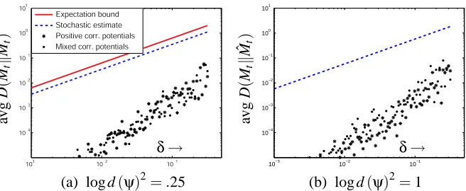
Applying these approximations to graphs with cycles, and following the same development used for constructing the strict bounds of Section 5, we find the following estimates of steady-state error. Note that, other than those outlined in the previous section (and described in Appendix B), this development involves no additional approximations.
Approximation 23. After n≥1 iterations of loopy BP subject to additional errors at each iteration of magnitude (measured by
D
) bounded above by some constant δ, with initial messages {m0tu}
satisfying
D
(mtukm0tu)less than some constant C, results in an expected KL-divergence between a
true BP fixed point{Mt}and the approximation{Mˆtn}bounded by
Ey
D(MtkMˆtn)
=Ey
h
D
(M
tkM
ˆ n t )i
≤
∑
u∈Γt
((1−γut)εn−1ut +δ)
whereεts0 =C and
εi
ts=
∑
u∈Γt\s((1−γut)εi−1ut +δ).
Comment. The argument proceeds similarly to that of Theorem 15. Let εits bound the quantity