Sparse Semi-supervised Learning Using Conjugate Functions

Sparse Semi-supervised Learning Using Conjugate Functions

Shiliang Sun [email protected]

Department of Computer Science and Technology East China Normal University

500 Dongchuan Road, Shanghai 200241, P. R. China

John Shawe-Taylor [email protected]

Department of Computer Science University College London

Gower Street, London WC1E 6BT, United Kingdom

Editor: Tony Jebara

Abstract

In this paper, we propose a general framework for sparse semi-supervised learning, which concerns using a small portion of unlabeled data and a few labeled data to represent target functions and thus has the merit of accelerating function evaluations when predicting the output of a new example. This framework makes use of Fenchel-Legendre conjugates to rewrite a convex insensitive loss involving a regularization with unlabeled data, and is applicable to a family of semi-supervised learning methods such as multi-view co-regularized least squares and single-view Laplacian sup-port vector machines (SVMs). As an instantiation of this framework, we propose sparse multi-view SVMs which use a squaredε-insensitive loss. The resultant optimization is an inf-sup problem and the optimal solutions have arguably saddle-point properties. We present a globally optimal iterative algorithm to optimize the problem. We give the margin bound on the generalization error of the sparse multi-view SVMs, and derive the empirical Rademacher complexity for the induced func-tion class. Experiments on artificial and real-world data show their effectiveness. We further give a sequential training approach to show their possibility and potential for uses in large-scale problems and provide encouraging experimental results indicating the efficacy of the margin bound and em-pirical Rademacher complexity on characterizing the roles of unlabeled data for semi-supervised learning.

Keywords: semi-supervised learning, Fenchel-Legendre conjugate, representer theorem, multi-view regularization, support vector machine, statistical learning theory

1. Introduction

Semi-supervised learning, considering how to estimate a target function from a few labeled exam-ples and a large quantity of unlabeled examexam-ples, is one of currently active research directions. If the unlabeled data are properly used, it can get a superior performance over the counterpart supervised learning approaches. For an overview of semi-supervised learning methods, refer to Chapelle et al. (2006) and Zhu (2008).

automatic programs, but needs a high cost to label them manually. Theoretical results on semi-supervised learning include PAC-analysis (Balcan and Blum, 2005), manifold regularization (Belkin et al., 2006), and multi-view regularization theories (Sindhwani and Rosenberg, 2008), etc.

Among the methods proposed for semi-supervised learning, a family of them, for example, Laplacian regularized least squares (RLS), Laplacian support vector machines (SVMs), Co-RLS, Co-Laplacian RLS, Co-Laplacian SVMs, and manifold co-regularization (Belkin et al., 2006; Sind-hwani et al., 2005; SindSind-hwani and Rosenberg, 2008), make use of the following representer theorem (Kimeldorf and Wahba, 1971) to represent the target function in a reproducing kernel Hilbert space (RKHS).

Theorem 1 (Representer theorem) Let

H

be an RKHS with kernel k :

X

×

X

→R. Fix any

func-tion V : Rn→R and any nondecreasing functionΨ: R→R. Define

J(f) =V(f(x1), ...,f(xn)) +Ψ(kfk2),

and linear space

L

=span_{k(x1,·), ...,k(xn,·)}. Then for any f∈

H

we have J(fL)≤J(f)with fL

being the projection of f onto

L

in the following form

fL= n

∑

i=1

αik(xi,·).

Thus if J∗=minfJ(f)exists, this minimum is attained for some f ∈

L

. Moreover, ifΨis strictly

increasing, each minimizer of J(f)over

H

must be contained in

L

.

Generally, in the objective function J(f) of these semi-supervised learning methods, labeled examples are used to calculate an empirical loss of the target function and simultaneously unlabeled examples are used for some regularization purpose. By the representer theorem, the target function would involve kernel evaluations on all the labeled and unlabeled examples. This is computationally undesirable, because for semi-supervised learning usually a considerably large number of unlabeled examples are available. Consequently, sparsity in the number of unlabeled data used to represent target functions is crucial, which constitutes the focus of this paper.

However, little work has been done on this theme. In particular, there is no unified framework proposed yet to deal with this sparsity concern. While the sparse Laplacian core vector machines (Tsang and Kwok, 2007) touched this problem, it has a complicated optimization and is not generic enough to generalize to other similar semi-supervised learning methods. In contrast with this, the technique developed in this paper, based on Fenchel-Legendre conjugates, is computationally sim-ple and widely applicable.

As far as multi-view learning is concerned there has been work that introduces sparsity of the unlabeled data into the representation of the classifiers (Szedmak and Shawe-Taylor, 2007). This builds on the ideas developed for two view learning known as the SVM-2K (Farquhar et al., 2006). The approach adopted is the use of an ε-insensitive loss function for the similarity constraint be-tween the two functions from two views. Unfortunately the resulting optimization is somewhat unmanageable and only scales to small-scale data sets despite interesting theoretical bounds that show the improvement gained using the unlabeled data.

views and shows that this problem can be solved implicitly with variables only indexed by the la-beled data. To compute the value of this function on new data would still require a non-sparse dual representation in terms of the unlabeled data. However, we show that through optimizing weights of the unlabeled data the solution of the l2problem converges to the solution of anε-insensitive prob-lem ensuring that we subsequently obtain sparsity in the unlabeled data. Furthermore, we develop the generalization analysis of Szedmak and Shawe-Taylor (2007) to this case giving computable expressions for the corresponding empirical Rademacher complexity.

To show the application of Fenchel-Legendre conjugates, in Section 2 we propose a novel sparse semi-supervised learning approach: sparse multi-view SVMs, where the conjugate functions play a central role in reformulating the optimization problem. The dual optimization of a subroutine of the sparse multi-view SVMs is converted to a quadratic programming problem in Section 3 whose scale only depends on the number of labeled examples, indicating the advantages of using conjugate functions. The generalization error of the sparse multi-view SVMs is given in Section 4 in terms of Rademacher complexity theory, followed by a derivation of empirical Rademacher complexity of the class of functions induced by this new method in Section 5. Section 6 reports experimental results of the sparse multi-view SVMs, comparisons with related methods, and the possibility and potential for large-scale applications through sequential training. Extensions of the use of conju-gate functions to a general convex loss and other related semi-supervised learning approaches are discussed in Section 7. Finally, Section 8 concludes this paper.

2. Sparse Multi-view SVMs

Multi-view semi-supervised learning, an important branch of semi-supervised learning, combines different sets of properties of an example to learn a target function. These different sets of prop-erties are often referred to as views. Typical applications of multi-view learning are web-page cat-egorization and content-based multimedia information retrieval. In web-page catcat-egorization, each web-page can be simultaneously described by disparate properties such as main text, inbound and outbound hyper-links. In content-based multimedia information retrieval, a multimedia segment can include both audio and video components. For such scenarios learning with multiple views is usually very beneficial. Even for problems with no natural multiple views, artificially generated views can still work favorably (Nigam and Ghani, 2000).

A useful assumption for multi-view learning is that features from each view are sufficient to train a good learner (Blum and Mitchell, 1998; Balcan et al., 2005; Farquhar et al., 2006). Making good use of this assumption through collaborative training or regularization between views can remove many false hypotheses from the hypothesis space, and thus facilitates effective learning.

For multi-view learning, an input x consists of multiple components from different views, for example, x= (x1, . . . ,xm) for an m-view representation. A function fj defined on view j only

depends on xj_{, that is f}

j(x):= fj(xj). Suppose we have a set ofℓlabeled examples {(xi,yi)}ℓi=1 with yi∈ {1,−1}, and a set of u unlabeled examples{xi}ℓ_i=+_ℓu₊₁. The objective function of our sparse

more than two views.

min

f1∈H1,f2∈H2

1 2ℓ

ℓ

∑

i=1

[(1₋yif1(xi))++ (1−yif2(xi))+] +

γn(kf1k2+kf2k2) +γv

ℓ+u

∑

i=1

(_|f1(xi)−f2(xi)| −ε)2+, (1)

where nonnegative scalarsγn,γvare respectively norm regularization and multi-view regularization

coefficients, and the last term is an ε-insensitive loss between two views with function (_·)+ :=

max(0,_·)being the hinge loss. The final classifier for predicting the label of a new example is

fc(x) =sgn

f1(x) +f2(x) 2

. (2)

In the rest of this section, we will show that the use of the ε-insensitive loss indeed enforces sparsity, and Fenchel-Legendre conjugates can be adopted to reformulate the optimization problem. We also show the saddle-point properties for optimal solutions and give a (globally optimal) iterative optimization algorithm.

2.1 Sparsity

In order to show the role of theε-insensitive loss for sparsity pursuit, here we represent f1(x)and f2(x)in feature spaces as

f1(x) =w⊤1φ1(x) +b1, f2(x) =w⊤2φ2(x) +b2,

whereφi(x) (i=1,2)is the image of x in feature spaces. Problem (1) can be rewritten as

min

w1,w2,ξ1,ξ2,b1,b2

P0= 1 2ℓ

ℓ

∑

i=1

(ξi₁+ξi₂) +γn(kw1k2+kw2k2) +

γv

ℓ+u

∑

i=1

(_|w⊤₁φ1(xi) +b1−w⊤2φ2(xi)−b2| −ε)2+

s.t.







yi(w⊤1φ1(xi) +b1)≥1−ξi₁,

yi(w⊤2φ2(xi) +b2)≥1−ξi2,

ξi

1, ξi2≥0, i=1, . . . , ℓ , whereξ₁:= [ξ1

1, . . . ,ξℓ1]andξ2:= [ξ12, . . . ,ξℓ2]. The Lagrangian is

L= P0− ℓ

∑

i=1 [λi

1(yi(w⊤1φ1(xi) +b1)−1+ξi1) +

λi

2(yi(w⊤2φ2(xi) +b2)−1+ξi2) +νi1ξi1+νi2ξi2], whereλi₁,λi

2,νi1,νi2≥0(i=1, . . . , ℓ)are Lagrange multipliers.

Suppose w1_∗, w2_∗are the optimal solutions. By the KKT conditions, the optimal solutions w1_∗ should satisfy _∂∂_wL

1∗ =0. Therefore, we get

w1∗=−γ_γv

n

ℓ+u

∑

i=1

(_|w⊤₁φ1(xi) +b1−w⊤2φ2(xi)−b2| −ε)+φ˜i+

1 2γn

ℓ

∑

i=1

λi

where we suppose the derivative exists everywhere and ˜φi :=sgn{w⊤1φ1(xi) +b1−w⊤2φ2(xi)−

b2_}φ1(xi). Now we can assess the sparsity of problem (1). From the above equation, w1_∗ is the

linear combination of labeled examples withλi₁>0, and those unlabeled examples on which the difference of predictions from two views exceedsε. In this sense, we can get sparse solutions by providing a non-zeroε. Similar analysis applies to w2_∗. Therefore, function f(x)is sparse in the number of used unlabeled examples. This analysis on sparsity is also well justified by the represen-ter theorem.

2.2 Reformulation Using Conjugate Functions

Define ti:= [f1(xi)−f2(xi)]2. Then theε-insensitive loss term can be written as

fε(t) = ℓ+u

∑

i=1

(√ti−ε)2+, (3)

where vector t := [t1, . . . ,tℓ+u]⊤. We give a theorem affirming the convexity of function fε(t).

Theorem 2 Function fε(t)defined by (3) is convex.

Proof First, we show that f_ε(ti):= (√ti−ε)2+ with a convex domain [0,+∞) is convex. When

ti ∈(ε2,+∞), the second derivative ∇2fε(ti) = 1₂εti−3/2≥0. Thus, function fε(ti) is convex for

ti∈(ε2,+∞). Moreover, the value of function fε(ti)for ti∈(ε2,+∞)is larger than 0 which is the

value of fε(ti)for ti∈[0,ε2], and function fε(ti) with domain[0,+∞) is continuous atε2. Hence,

f_ε(ti)is convex on the domain[0,+∞).

Then, being a nonnegative weighted sum of convex functions, f_ε(t)is indeed convex.

Define conjugate vector z= [z1, . . . ,zℓ+u]⊤with entries being conjugate variables. The

Fenchel-Legendre conjugate (which is also often called convex conjugate or conjugate function) f_ε∗(z)is

f_ε∗(z) = sup

t∈dom fε

(t⊤z₋f_ε(t)) =sup

t

ℓ+u

∑

i=1

[ziti−(√ti−ε)2+] =

ℓ+u

∑

i=1 sup

ti

[ziti−(√ti−ε)2+].

The domain of the conjugate function consists of z_∈Rℓ+ufor which the supremum is finite (i.e., bounded above) (Boyd and Vandenberghe, 2004). Define

f_ε∗(zi) =sup ti

[ziti−(√ti−ε)2+]. (4)

Then, f_ε∗(z) =∑ℓ_i=+₁uf_ε∗(zi). As a pointwise supremum of a family of affine functions, f_ε∗(zi) is

convex. Being a nonnegative weighted sum of convex functions, f_ε∗(z)is also convex. Below we derive the formulation of f_ε∗(zi).

Theorem 3 Function f_ε∗(zi)defined by (4) has the following form

f_ε∗(zi) =

(

ziε2

1−zi, for 0<zi<1

0, for zi≤0.

Proof By definition, we have

f_ε∗(zi) =max ti

(

sup 0≤ti≤ε2

ziti,sup ti>ε2

[ziti−(√ti−ε)2]

)

. (6)

The value of function sup_0≤ti≤ε2z_it_iis simple to characterize. We now characterize the second term

sup_ti>ε2[z_it_i−(√t_i−ε)2] =sup_t

i>ε2(ziti−ti−ε

2₊₂ε√_t

i). For 0<zi<1, we let the first derivative

equal to zero to find the supremum. For zi≤0 or zi≥1 the derivative does not exist and thus we

use function values at end points to find the supremum. As a result, we have

sup

ti>ε2

[ziti−(√ti−ε)2] =



 

 

ziε2

1−zi, for 0<zi<1

ziε2, for zi≤0

+∞, for zi≥1.

According to (6) and further removing the range where f_ε∗(zi)is unbounded above, we reach the

conjugate given in (5).

Now the Fenchel-Legendre conjugate f_ε∗(z) can be represented by∑_iℓ₌+₁uf_ε∗(zi), which is also

well justified by the following theorem.

Theorem 4 (Boyd and Vandenberghe, 2004) Ifϕ(u,v) =ϕ1(u) +ϕ2(v), whereϕ1andϕ2are in-dependent convex functions (inin-dependent means they are functions of different variables) with con-jugatesϕ∗₁andϕ∗₂, respectively, then

ϕ∗_{(ω,z) =ϕ}∗

1(ω) +ϕ∗2(z).

A nice property of the conjugate function is on the conjugate of the conjugate, which is central to the reformulation of our optimization problem. This property is stated by Lemma 5.

Lemma 5 (Rifkin and Lippert, 2007) If function f is closed, convex, and proper, then the

conju-gate function of the conjuconju-gate is itself, that is, f∗∗= f , where we have defined function f is closed if its epigraph is closed, and f is proper if dom f ₆=/0and f>₋∞.

It is true that function f_ε(t) is closed and proper. Moreover, we have proved the convexity of f_ε(t)in Theorem 2. Therefore, we can use Lemma 5 to get the following equality

fε(t) =sup

z

(z⊤t₋f_ε∗(z)). (7)

That is

ℓ+u

∑

i=1

(√ti−ε)2+=sup

z

(z⊤t₋f_ε∗(z)) =sup

z

ℓ+u

∑

i=1

[ziti−fε∗(zi)].

By (7), we have

ℓ+u

∑

i=1

(_|f1(xi)−f2(xi)| −ε)2+=

ℓ+u

∑

i=1

(√ti−ε)2+=sup

z

ℓ+u

∑

i=1

Therefore, the objective function for sparse multi-view SVMs becomes

min

f1∈H1,f2∈H2

1 2ℓ

ℓ

∑

i=1

[(1₋yif1(xi))++ (1−yif2(xi))+] +

γn(kf1k2+kf2k2) +γvsup z

ℓ+u

∑

i=1

{zi[f1(xi)−f2(xi)]2−f_ε∗(zi)}. (8)

As an application of Theorem 1, the solution to problem (8) has the following form

f1(x) = ℓ+u

∑

i=1

αi

1k1(xi,x), f2(x) =

ℓ+u

∑

i=1

αi

2k2(xi,x). (9)

Applying the reproducing properties of kernels, we get

kf1k2_=α⊤

1K1α1,kf2k2=α⊤2K2α2,

where K1and K2are(ℓ+u)_×(ℓ+u)Gram matrices from two views

V

1_and

_V

2_{, respectively, and} vectorα1= (α11, ...,αℓ1+u)⊤,α2= (α12, ...,αℓ2+u)⊤. Moreover, we have

f1=K1α1,f2=K2α2,

with f1 := (f1(x1), ...,f1(xℓ+u))⊤, f2 := (f2(x1), ...,f2(xℓ+u))⊤. Define diagonal matrix

U =diag(z1, . . . ,zℓ+u) with every element taking values in the range [0,1). Problem (8) can be

reformulated as

min α1,α2,ξ1,ξ2,b1,b2

sup z 1 2ℓ ℓ

∑

i=1

(ξi₁+ξi₂) +γn(α1⊤K1α1+α⊤2K2α2) +

γv[(K1α1−K2α2)⊤U(K1α1−K2α2)− ℓ+u

∑

i=1 f_ε∗(zi)]

s.t.     

yi(∑ℓj+=u1α

j

1k1(xj,xi) +b1)≥1−ξi1, yi(∑ℓ_j+₌u₁α₂jk2(xj,xi) +b2)≥1−ξi2,

ξi

1, ξi2≥0, i=1, . . . , ℓ .

(10)

2.3 Saddle-Point Property

We present a theorem concerning the convexity and concavity of optimization problem (10).

Theorem 6 The objective function in problem (10) is convex with respect toα1,α2,ξ1,ξ2, b1, and b2, and concave with respect to z.

Proof First, we show the convexity. The standard form of this optimization problem is

min α1,α2,ξ1,ξ2,b1,b2

sup z 1 2ℓ ℓ

∑

i=1 (ξi

1+ξi2) +γn(α⊤1K1α1+α⊤2K2α2) +

γv[(K1α1−K2α2)⊤U(K1α1−K2α2)− ℓ+u

∑

i=1 f_ε∗(zi)]

s.t.     

−yi(∑ℓj+=u1α

j

1k1(xj,xi) +b1) +1−ξi1≤0,

−yi(∑ℓ_j+₌u₁α₂jk2(xj,xi) +b2) +1−ξi₂≤0, −ξi

This problem involves one objective function and three sets of inequality constraint functions (on the left hand side of each inequality). Clearly, the domain of each objective and constraint function is a convex set. Now it suffices to prove the convexity of this problem by assessing the convexity of these functions. As all constraint functions are affine, they are convex. Then, we use the second-order condition, positive semidefinite property of a function’s Hessian or second derivative to judge the convexity of the objective function (Boyd and Vandenberghe, 2004). According to this condition, the first two items of the objective function are clear to be convex. The third part can be rewritten as

(K1α1−K2α2)⊤U(K1α1−K2α2) =kU1/2 K1 −K2

α

1

α2

k2,

which is a convex function k · k2 _{composed with an affine mapping and thus also convex (Boyd} and Vandenberghe, 2004). Being a nonnegative weighted sums of convex functions, the objective function is therefore convex with respect toα1,α2,ξ1,ξ2,b1,b2.

Then, we show the concavity using (8). As f_ε∗(zi)is convex, zi[f1(xi)−f2(xi)]2−f_ε∗(zi)is

con-cave with respect to zi. The concavity of∑ℓ_i=+₁u{zi[f1(xi)−f2(xi)]2−f_ε∗(zi)}follows from the fact

that a nonnegative weighted sum of concave functions is concave (Boyd and Vandenberghe, 2004). Hence, the objective function in problem (10) is concave with respect to z.

Letθdenote the parametersα1,α2,ξ1,ξ2,b1,b2. We can simply denote the above optimization problem as

inf θ supz

f(θ,z) (11)

associated with constraints on the labeled examples, where f(θ,z)is convex with respect toθ, and concave with respect to z. We give the following theorem on the equivalence of swapping the infimum and supremum for our optimization problem and include a proof for completeness.

Theorem 7 (Boyd and Vandenberghe, 2004) If f(θ,z) with domain Θ and Z is convex with re-spect toθ_∈Θ, and concave with respect to z_∈Z, the following equality holds

inf θ supz

f(θ,z) =sup z

inf θ f(θ,z)

under some slight assumptions.

Proof The idea is first to represent the left-hand side as a value of a convex function, and then

show that the conjugate of its conjugate is equal to the right-hand side when the same input value is plugged in Boyd and Vandenberghe (2004).

The left-hand side can be expressed as p(0), where

p(u) =inf θ supz

[f(θ,z) +u⊤z].

It is not difficult to show that p is a convex function. Being a pointwise supremum of convex function f(θ,z)+u⊤z, sup_z[f(θ,z)+u⊤z]is a convex function of(θ,u). Because sup_z[f(θ,z)+u⊤z] is convex with respect to(θ,u), we have p(u)is convex.

The Fenchel-Legendre conjugate of p(u)is

p∗(v) =sup

u

[u⊤v₋inf θ supz

which would be+∞if z6=v. Therefore,

p∗(v) =

−inf_θ f(θ,v), for v_∈Z +∞, otherwise.

The conjugate of p∗(z)is given by

p∗∗(u) =sup

z_∈Z

(u⊤z₋p∗(z)) =sup

z_∈Z

(u⊤z+inf

θ f(θ,z)) =supz

inf

θ [f(θ,z) +u⊤z].

Suppose 0_∈domp(u)and p(u)is closed and proper. Then by Lemma 5 we have p(0) =p∗∗(0) which completes the proof.

Now we give a theorem showing that the optimal pair ˜θ, ˜z is a saddle-point.

Theorem 8 If the following equality holds for function f(θ,z)

inf θ supz

f(θ,z) =sup z

inf

θ f(θ,z) = f(θ˜,˜z),

then the optimal pair ˜θ, ˜z forms a saddle-point.

Proof From the given equality, we have

inf θ supz

f(θ,z) =sup

z

f(_θ˜_{,z) = f(θ}˜_,˜z),

and

sup

z

inf

θ f(θ,z) =infθ f(θ,˜z) =f(θ˜,˜z),

Therefore,

f(θ˜,z)_≤ f(θ˜,˜z)_≤ f(θ,˜z),

which indeed satisfies the definition of a saddle-point. The proof is completed.

2.4 Iterative Optimization Algorithm

To solve the optimization problem sup_zinf_θf(θ,z)which is respectively concave and convex with respect to z andθ, we give an algorithm with guaranteed convergence by the following theorem.

Theorem 9 Given an initial value z0for z, solve infθf(θ,z0)and obtain the global optimal pointθ0. Then we find arg maxzf(θ0,z)to get z1from which we can getθ1as a result of optimize infθf(θ,z1). Repeat this process until a convergence point(θˆ,ˆz)is reached. Suppose ˜θ, ˜z is a saddle point. We have f(θˆ,ˆz) = f(θ˜,˜z). That is, we got the optimal values of the objective function. If f is strictly concave and strictly convex with respect to the variables, we further have ˆθ=θ˜ and ˆz=˜z.

Proof According to the properties of function f and the algorithm procedure, we know that the

convergence point is a saddle point. Thus, we have

By the saddle-point property of(_θ˜_{,˜z), we have}

f(θ˜,˜z)_≥f(θ˜,ˆz),

and

f(θ˜,˜z)_≤f(θˆ,˜z).

Therefore, the above inequalities should hold with equalities and we have f(θ˜,˜z) = f(θˆ,ˆz). Fur-thermore, if f is strictly concave and strictly convex with respect to the variables, it is true that ˆθ=θ˜ and ˆz=˜z.

On solving arg maxzf(θ,z) required in Theorem 9, we can maximize the term related to z,

namely z⊤t₋f_ε∗(z) =∑_iℓ₌+₁u[ziti−f_ε∗(zi)]. For this purpose, we have the following theorem. Theorem 10

sup

zi∈dom fε∗(zi)

[ziti−f_ε∗(zi)] = (√ti−ε)2+,

and

arg sup

zi∈dom fε∗(zi)

[ziti−fε∗(zi)] =

(

1₋√ε_t

i, for ti>ε

2 0, for 0_≤ti≤ε2.

Without loss of generality, we can confine the range of zito[0,1).

Proof We have

sup

zi∈dom fε∗(zi)

[ziti−f_ε∗(zi)] =max zi {

sup 0<zi<1

ziti−

ziε2

1₋zi

,sup

zi≤0

ziti}.

The first supremum can be solved by setting the derivative with respect to zito zero. We have

sup 0<zi<1

ziti−

ziε2

1₋zi

= (√ti−ε)2

where ti>ε2, and the supremum is attained with zi=1−√ε_t i.

When ti<0, supzi≤0ziti is unbounded above. When 0≤ti≤ε

2_{, sup}

zi≤0ziti=0 with the

supre-mum attained at zi =0. Therefore, maxzi{sup0<zi<1ziti− ziε2

1−zi,supzi≤0ziti}= ( √

ti−ε)2+ with the

supremum attained when zi∈[0,1), which completes the proof.

For sparsity pursuit, during each iteration we remove those unlabeled examples whose cor-responding zi’s are zero. By the representer theorem, this would not influence the value of the

3. Dual Optimization

According to the iterative optimization algorithm, when optimizing problem (10), we start from an initial value z0and then solveθ0. In this section, we show how to solve this subroutine with fixed z.

Now the optimization problem is equivalent to

min α1,α2,ξ1,ξ2,b1,b2

F0= 1 2ℓ

ℓ

∑

i=1

(ξi₁+ξi₂) +γn(α⊤1K1α1+α⊤2K2α2) +

γv(K1α1−K2α2)⊤U(K1α1−K2α2)

s.t.



 

 

yi(∑ℓj+=u1α

j

1k1(xj,xi) +b1)≥1−ξi1, yi(∑ℓ_j+₌u₁α₂jk2(xj,xi) +b2)≥1−ξi₂, ξi

1, ξi2≥0, i=1, . . . , ℓ .

(12)

3.1 Lagrange Dual Function

We will solve problem (12) through optimizing its dual problem which is simpler to solve. Now we derive its Lagrange dual function.

Suppose λi₁,λi

2,νi1,νi2≥0 (i=1, . . . , ℓ) be the Lagrange multipliers associated with the in-equality constraints. Defineλj= [λ1j, . . . ,λℓj]⊤ andνj= [ν1j, . . . ,νℓj]⊤ (j=1,2). The Lagrangian

L(α1,α2,ξ1,ξ2,b1,b2,λ1,λ2,ν1,ν2)can be written as L= F0−

ℓ

∑

i=1 [λi₁(yi(

ℓ+u

∑

j=1

αj

1k1(xj,xi) +b1)−1+ξi1) +

λi

2(yi(

ℓ+u

∑

j=1

αj

2k2(xj,xi) +b2)−1+ξi2) +νi1ξi1+νi2ξi2]. Note that

(K1α1−K2α2)⊤U(K1α1−K2α2)

= α⊤₁K1U K1α1−2α⊤1K1U K2α2+α⊤2K2U K2α2.

To obtain the Lagrangian dual function, L has to be minimized with respect to the primal variablesα1,α2,ξ1,ξ2,b1,b2. To eliminate these variables, we compute the corresponding partial derivatives and set them to 0, obtaining the following conditions

2J1α1−2γvK1U K2α2=Λ1, (13) 2J2α2−2γvK2U K1α1=Λ2, (14)

λi

1+νi1= 1

2ℓ, (15)

λi

2+νi2= 1

2ℓ, (16)

ℓ

∑

i=1

λi

1yi=0,

ℓ

∑

i=1

λi

where

J1 := γnK1+γvK1U K1,

J2 := γnK2+γvK2U K2,

Λ1 := ℓ

∑

i=1

λi

1yiK1(:,i), Λ2 :=

ℓ

∑

i=1

λi

2yiK2(:,i),

with K1(:,i)and K2(:,i)being the ith column of the corresponding Gram matrices.

Substituting (13)_∼(17) into L results in the following expression of the Lagrangian dual function gL(λ1,λ2,ν1,ν2)

gL = γn(α⊤1K1α1+α⊤2K2α2) +γv(α⊤1K1U K1α1−2α⊤1K1U K2α2+

α⊤

2K2U K2α2)−α⊤1Λ1−α⊤2Λ2+ ℓ

∑

i=1

(λi₁+λi₂)

= 1

2α

⊤

1Λ1+ 1 2α

⊤

2Λ2−α⊤1Λ1−α⊤2Λ2+ ℓ

∑

i=1

(λi₁+λi₂)

= ₋1 2α

⊤

1Λ1− 1 2α

⊤

2Λ2+ ℓ

∑

i=1 (λi

1+λi2). (18)

We obtain the following from (13) and (14)

α1= 1 2J

−1

1 (Λ1+2γvK1U K2α2) (19)

α2= 1 2J

−1

2 (Λ2+2γvK2U K1α1). (20) From (13) and (20), we have

(2J1−2γ2_vK1U K2J₂−1K2U K1)α1=Λ1+γvK1U K2J2−1Λ2.

Define M1 =2J1₋2γ2_vK1U K2J₂−1K2U K1. Suppose the above linear system is well-posed (if ill-posed we can employ approximate numerical analysis techniques). We get

α1=M1−1(Λ1+γvK1U K2J2−1Λ2). From (14) and (19), we have

(2J2₋2γ2_vK2U K1J₁−1K1U K2)α2=Λ2+γvK2U K1J₁−1Λ1. Define M2=2J2₋2γ2_vK2U K1J₁−1K1U K2. Thus we get

Now withα1andα2substituted into (18), the Lagrange dual function gL(λ1,λ2,ν1,ν2)is

gL = inf

α1,α2,ξ1,ξ2,b1,b2

L=₋1 2α

⊤

1Λ1− 1 2α

⊤

2Λ2+ ℓ

∑

i=1 (λi

1+λi2) = ₋1

2(Λ1+γvK1U K2J

−1

2 Λ2)⊤M− 1 1 Λ1−

1 2(Λ2+

γvK2U K1J1−1Λ1)⊤M2−1Λ2+ ℓ

∑

i=1 (λi

1+λi2).

3.2 Solving the Dual Problem

The Lagrange dual problem is given by

max λ1,λ2

gL s.t.       

0_≤λi_1≤2ℓ1, i=1, . . . , ℓ 0_≤λi_2≤2ℓ1, i=1, . . . , ℓ

∑ℓ

i=1λi1yi=0, ∑ℓ

i=1λi2yi=0.

As Lagrange dual functions are always concave (Boyd and Vandenberghe, 2004), we can formulate the above problem as a convex optimization problem

min λ1,λ2 −

gL s.t.       

0_≤λi_1≤2ℓ1, i=1, . . . , ℓ 0_≤λi_2≤2ℓ1, i=1, . . . , ℓ

∑ℓ

i=1λi1yi=0, ∑ℓ

i=1λi2yi=0.

(21)

Define matrix Y =diag(y1, . . . ,yℓ). Then,Λ1=Kℓ1Yλ1andΛ2=Kℓ2Yλ2with Kℓ1=K1(:,1 :ℓ) and Kℓ2=K2(:,1 :ℓ). We have

−gL =

1

2(Λ1+γvK1U K2J

−1

2 Λ2)⊤M1−1Λ1+ 1 2(Λ2+

γvK2U K1J₁−1Λ1)⊤M₂−1Λ2− ℓ

∑

i=1

(λi₁+λi₂)

= 1

2(λ

⊤

1 λ⊤2)

A B C D λ 1 λ2

−1⊤(λ1+λ2), where

A := Y K_ℓ1⊤M−₁1Kℓ1Y,

and 1= (1, . . . ,1(ℓ))⊤.

Substituting M1and M2into the expressions of B and C, we can prove that B=C⊤. In addition,

because of the convexity of function₋g, we affirm that matrix

A B C D

is positive semi-definite.

Hence, the optimization problem in (21) can be rewritten as

min λ1,λ2

1 2(λ

⊤

1 λ⊤2)

A B C D

λ

1

λ2

−1⊤(λ1+λ2)

s.t.



  

  

0λ1_2l11, 0λ2_2l11,

λ⊤

1y=0,

λ⊤

2y=0,

where y= (y1, . . . ,yℓ)⊤. After solving this problem using standard software, we then obtainνi1and

νi

2by (15) and (16).

We now state the advantages of optimizing this dual problem over optimizing the primal prob-lem (12):

• Less optimization variables as for typical semi-supervised learningℓ_≪u, and

• Simpler constraint functions.

The solution of bias terms b1 and b2 can be obtained through support vectors. Due to KKT conditions, the following equalities hold

λi

1(yi(

ℓ+u

∑

j=1

αj

1k1(xj,xi) +b1)−1+ξ

i

1) =0,

λi

2(yi(

ℓ+u

∑

j=1

αj

2k2(xj,xi) +b2)−1+ξi2) =0,

νi

1ξi1=0,

νi

2ξi2=0, i=1, . . . , ℓ.

For support vectors xi, we haveνij >0 (and thusξij =0) andλij>0(j=1,2). Therefore, we can

resolve the bias terms by averaging yi(∑ℓ_j+₌u₁α₁jk1(xj,xi) +b1)−1=0 and yi(∑ℓ_j+₌₁uα₂jk2(xj,xi) +

b2)−1=0 over all support vectors.

3.3 Advantages of Using Conjugate Functions

The primal problem can be rewritten as

min α1,α2,ξ1,ξ2,b1,b2,δi

D0= 1 2ℓ

ℓ

∑

i=1

(ξi₁+ξi₂) +γn(α⊤1K1α1+α⊤2K2α2) +γv

ℓ+u

∑

i=1

δ2 i s.t.             

yi(∑ℓj+=u1α

j

1k1(xj,xi) +b1)≥1−ξi1, i=1, . . . , ℓ , yi(∑ℓ_j+₌u₁α₂jk2(xj,xi) +b2)≥1−ξi₂, i=1, . . . , ℓ , ξi

1, ξi2≥0, i=1, . . . , ℓ , (∑ℓ_j+₌u₁α₁jk1(xj,xi) +b1)−(∑lj+=u1α

j

2k2(xj,xi) +b2)≥ −δi−ε, i=1, . . . , ℓ+u,

(∑ℓ_j+₌u₁α₁jk1(xj,xi) +b1)−(∑l_j+₌u₁α₂jk2(xj,xi) +b2)≤δi+ε, i=1, . . . , ℓ+u,

(22)

where yi∈ {1,−1},γn,γv≥0.

We will solve problem (22) through optimizing its dual problem which can be simpler to solve. Supposeλi₁,λi

2,νi1,νi2≥0(i=1, . . . , ℓ)and µi1,µi2(i=1, . . . , ℓ+u)are the Lagrange multipliers asso-ciated with the inequality constraints of problem (22). Defineδ= [δ1, . . . ,δℓ+u]⊤,λj= [λ1j, . . . ,λℓj]⊤, νj = [ν1j, . . . ,νℓj]⊤, and µj = [µ1j, . . . ,µℓj+u]⊤ (j = 1,2). The Lagrangian

L(α1,α2,ξ1,ξ2,b1,b2,δ,λ1,λ2,ν1,ν2,µ1,µ2)can be written as

L= D0− ℓ

∑

i=1 [λi

1(yi(

ℓ+u

∑

j=1

αj

1k1(xj,xi) +b1)−1+ξi1) +

λi

2(yi(

ℓ+u

∑

j=1

αj

2k2(xj,xi) +b2)−1+ξi2) +νi1ξi1+νi2ξi2]− ℓ+u

∑

i=1 µi₁[

ℓ+u

∑

j=1

αj

1k1(xj,xi) +b1− ℓ+u

∑

j=1

αj

2k2(xj,xi)−b2+δi+ε] + ℓ+u

∑

i=1 µi₂[

ℓ+u

∑

j=1

αj

1k1(xj,xi) +b1− ℓ+u

∑

j=1

αj

2k2(xj,xi)−b2−δi−ε].

derivatives and set them to 0, obtaining the following conditions

2γnK1α1= ℓ

∑

i=1

λi

1yiK1(:,i) + ℓ+u

∑

i=1

(µi₁₋µi₂)K1(:,i),

2γnK2α2= ℓ

∑

i=1

λi

2yiK2(:,i)− ℓ+u

∑

i=1

(µi₁₋µi₂)K2(:,i),

λi

1+νi1= 1

2ℓ, i=1, . . . , ℓ

λi

2+νi2= 1

2ℓ, i=1, . . . , ℓ

−

ℓ

∑

i=1

λi

1yi−

ℓ+u

∑

i=1 µi₁+

ℓ+u

∑

i=1

µi₂=0,

−

ℓ

∑

i=1

λi

2yi+

ℓ+u

∑

i=1 µi₁₋

ℓ+u

∑

i=1

µi₂=0, 2γvδi−µi1−µi2=0, i=1, . . . , ℓ+u.

Substituting these equations into the Lagrangian as what was done in Section 3.1, it is clear that finally L is a quadratic function involvingλ1,λ2,µ1,µ2. The dual optimization problem would be a quadratic optimization involving 2ℓ+2(ℓ+u)parameters. Now we see this direct optimization is indeed of large-scale and time-consuming.

4. Generalization Error

In this section, we analyze the generalization performance of the sparse multi-view SVMs making use of Rademacher complexity theory and the margin bound.

4.1 Rademacher Complexity Theory

Important background on Rademacher complexity theory (Bartlett and Mendelson, 2002; Shawe-Taylor and Cristianini, 2004) is introduced below.

Definition 11 For a sample S=_{x1, . . . ,xℓ}generated by a distribution

D

on a set

X

and a real-valued function class

F

with domain

X

, the empirical Rademacher complexity of

F

is the random variable

ˆ

Rℓ(

F

) =Eσ

"

sup

f∈F

2 ℓ ℓ

∑

i=1

σif(xi)

x1, . . . ,xℓ

#

,

where σ=_{σ1, . . . ,σℓ} are independent uniform {±1}-valued (Rademacher) random variables. The Rademacher complexity of

F

is

Rℓ(

F

) =ES[Rℓˆ (

F

)] =ESσ

"

sup

f_∈F

2 ℓ ℓ

∑

i=1

σif(xi)

# .

Lemma 12 Fixδ_∈(0,1)and let

F

be a class of functions mapping from an input space ˜

X

( ˜

X

=

D

. Then with probability at least 1−δover random draws of samples of sizeℓ, every f∈

F

satisfies

ED[f(x˜)] ≤ Eˆ[f(x˜)] +Rℓ(

F

) +

r

ln(2/δ) 2ℓ

≤ Eˆ[f(x˜)] +_Rˆ_ℓ(

_F

_{) +3}

r

ln(2/δ) 2ℓ ,

where ˆE[f(x˜)]is the empirical error averaged on theℓexamples.

4.2 Margin Bound for Sparse Multi-view SVMs

By (2), the prediction function of the sparse multi-view SVMs is derived from the average of pre-dictions from two views. Define the soft prediction function as

g(x) = 1

2(f1(x) +f2(x)).

We obtain the following margin bound regarding the generalization error of sparse multi-view SVMs. This bound is widely applicable to multi-view SVMs, for example, Szedmak and Shawe-Taylor (2007) independently provided a similar bound for the SVM-2K method.

Theorem 13 Fixδ_∈(0,1)and let

F

be the class of functions mapping from ˜

X

=

X

_×

Y

to R given by ˜f(x,y) =₋yg(x)where g=1

2(f1+f2)∈

G

and ˜f ∈

F

. Let S={(x1,y1),···,(xℓ,yℓ)}be drawn independently according to a probability distribution

D

. Then with probability at least 1₋δover samples of sizeℓ, every g_∈

G

satisfies

PD(y6=sgn(g(x)))≤

1 2ℓ

ℓ

∑

i=1 (ξi

1+ξi2) +2 ˆRℓ(

G

) +3

r

ln(2/δ) 2ℓ ,

whereξi₁:= (1₋yif1(xi))+,ξi2:= (1−yif2(xi))+. Function yif1(xi)and yif2(xi)are called margins.

Proof Let H(_·)be the Heaviside function that returns 1 if its argument is greater than 0 and zero otherwise. We have

PD(y6=sgn(g(x))) =ED[H(−yg(x))]. (23)

Consider a loss function

A

: R_→[0,1], given by

A

(a) =







1, if a_≥0; 1+a, if₋1_≤a_≤0; 0, otherwise.

By Lemma 12 and since function

A

₋1 dominates H₋1, we have (Shawe-Taylor and Cristianini, 2004)

ED[H(f˜(x,y))−1]≤ED[

A

(f˜(x,y))−1]

≤Eˆ[

A

(_f˜_{(x,y))−1] +R}ˆ_ℓ((

_A

_−1)◦

_F

_{) +3}

r

Therefore,

ED[H(f˜(x,y))]≤ Eˆ[

A

(f˜(x,y))] +Rˆℓ((

A

−1)◦

F

) +3

r

ln(2/δ) 2ℓ .

In addition, we have

ˆ

E[

A

(f˜(x,y))] _≤ 1

ℓ ℓ

∑

i=1

(1₋yig(xi))+

= 1

2ℓ ℓ

∑

i=1

(1₋yif1(xi) +1−yif2(xi))+

≤ ₂1_ℓ

ℓ

∑

i=1

[(1₋yif1(xi))++ (1−yif2(xi))+]

= 1

2ℓ ℓ

∑

i=1

(ξi₁+ξi₂),

whereξi₁denotes the amount by which function f1fails to achieve margin 1 for(xi,yi)andξi₂applies

similarly to function f2.

Since(

A

₋1)(0) =0, we can apply the Lipschitz condition (Bartlett and Mendelson, 2002) of function(

A

−1)to get

ˆ

Rℓ((

A

−1)◦

F

)≤2 ˆRℓ(

F

).

It remains to bound the empirical Rademacher complexity of the class

F

. With yi∈ {1,−1}, we have

ˆ

Rℓ(

F

) = Eσ[sup

f∈F|

2 ℓ

ℓ

∑

i=1

σif˜(xi,yi)|]

= Eσ[sup

g∈G|

2 ℓ

ℓ

∑

i=1

σiyig(xi)|]

= Eσ[sup

g∈G|

2 ℓ

ℓ

∑

i=1

σig(xi)|]

= Rℓˆ (

G

). (24)

Finally, combining (23)_∼(24) completes the proof.

5. Empirical Rademacher Complexity

Theorem 14 Suppose

S

=_γ1 n(K1ℓK

−1

1 K1ℓ⊤+K2ℓK2−1K2ℓ⊤),Θ=γ1nU

1/2

u (K1uK₁−1K1u⊤+K2uK2−1K2u⊤)U 1/2

u ,

J

= 1

γnU

1/2

u (K1uK1−1K1ℓ⊤−K2uK2−1K2ℓ⊤), where K1ℓ and K2ℓ are respectively the first ℓrows of the Gram matrices K1and K2, K1u and K2uare respectively the last u rows of matrix K1and K2, and Uuis the diagonal matrix including the last u diagonal elements (initially fixed zℓ+1, . . . ,zℓ+u) of U .

Then the empirical Rademacher complexity ˆRℓ(

G

)is bounded as √U_2ℓ ≤Rˆℓ(

G

)≤U_ℓ, where

U

2= tr(

S

)₋γvtr(

J

⊤(I+γvΘ)−1

J

)for the first iteration of sparse multi-view SVMs, and

U

2=tr(

S

)for

subsequent iterations.

The remainder of this section before Section 5.4 completes the proof of this theorem, which was partially inspired by Rosenberg and Bartlett (2007) for analyzing co-regularized least squares.

We use problem (8) to reason about ˆRℓ(

G

). As a result of fixed z, we can remove fε∗(zi)without

loss of generality to resolve f1 and f2. It is true that the loss function ˆL :

H

1×

H

2→[0,∞)with ˆL := 1

2ℓ∑ℓi=1[(1−yif1(xi))++ (1−yif2(xi))+]satisfies

ˆL(0,0) =1.

Let Q(f1,f2) denote the objective function in (8) with f_ε∗(zi) removed. Substituting in the trivial

predictors f1≡0 and f2≡0 gives the following upper bound min

f1,f2∈H1×H2

Q(f1,f2)≤Q(0,0) =ˆL(0,0) =1.

Since all terms of Q(f1,f2)are nonnegative, we conclude that any(f₁∗,f₂∗)minimizing Q(f1,f2) is contained in

ˆ

H

= _{(f1,f2):γn(kf1k2+kf2k2) +γv

ℓ+u

∑

i=ℓ+1

zi[f1(xi)−f2(xi)]2≤1}. (25)

Therefore, the final predictor is chosen from the function class

G

=_{x_→ 1

2[f1(x) +f2(x)]:(f1,f2)∈ ˆ

H

_}.

The complexity ˆRℓ(

G

)is

ˆ

Rℓ(

G

) =Eσ

"

sup

(f1,f2)∈Hˆ

1 ℓ

ℓ

∑

i=1

σi(f1(xi) +f2(xi))

#

. (26)

As it only depends on the values of function f1(_·)and f2(_·)on theℓlabeled examples, by the repro-ducing kernel property which says the projection of function f onto a closed subspace containing k(x,_·) has the same value at x as f itself does (Rosenberg and Bartlett, 2007) we can restrict the function class ˆ

H

to the span of labeled and unlabeled data and thus write it as

ˆ

H

= _{(f1,f2):γn(α⊤1K1α1+α⊤2K2α2) +

γv(K1uα1−K2uα2)⊤Uu(K1uα1−K2uα2)≤1} = _{(f1,f2):(α⊤1 α⊤2)N

α

1

α2

≤1_},

where K1u and K2uare respectively the last u rows of matrix K1 and K2, Uu is the diagonal matrix

including the last u diagonal elements of U , and

N :=γn

K1 0

0 K2

+γv

K_1u⊤

−K_2u⊤

5.1 Evaluating the Supremum in Euclidean Space

Since (f1,f2)_∈

H

ˆ implies(₋f1,₋f2)_∈

H

ˆ , we can drop the absolute sign in (26). Now we can write

ˆ

Rℓ(

G

) = 1

ℓEσ_α sup

1,α2∈Rℓ+u

{σ⊤K1ℓα1+σ⊤K2ℓα2:(α⊤1 α⊤2)N

α

1

α2

≤1_}

= 1

ℓEσ_α1,αsup_2∈Rℓ+u{ σ⊤_(K

1ℓK2ℓ)

α

1

α2

:(α⊤₁ α⊤₂)N

α

1

α2

≤1_}, (28)

where K1ℓ,K2ℓrepresent the firstℓrows of the Gram matrices K1and K2, respectively.

For a symmetric positive definite matrix M, it is simple to show that (Rosenberg and Bartlett, 2007)

sup α:α⊤_Mα≤1

v⊤α=_kM−1/2v_k.

Without loss of generality, suppose positive semi-definite matrix N in (28) is positive definite and thus has full rank. If N does not have full rank, we can use subspace decomposition to rewrite ˆRℓ(

G

) to obtain a similar representation. Thus, we can evaluate the supremum as described above to get

ˆ

Rℓ(

G

) =1

ℓEσkN

−1/2

K_1ℓ⊤ K_2ℓ⊤

σ_k.

5.2 Bounding ˆRℓ(

G

)above and below

We make use of the Kahane-Khintchine inequality (Latala and Oleszkiewicz, 1994), stated here for convenience, to bound ˆRℓ(

G

).

Lemma 15 For any vectors a1,···,an in a Hilbert space and independent Rademacher random

variablesσ1,···,σn, we have

1 2Ek

n

∑

i=1

σiaik2≤(Ek n

∑

i=1

σiaik)2≤Ek n

∑

i=1

σiaik2.

By Lemma 15 we have

U

√

2ℓ ≤Rˆℓ(

G

)≤

U

ℓ , (29)

where

U

2 ₌

EσkN−1/2

K_1ℓ⊤ K_2ℓ⊤

σ_k2

= _Eσtr[(K1ℓK2ℓ)N−1

K_1ℓ⊤ K_2ℓ⊤

σσ⊤_]

= tr[(K1ℓK2ℓ)N−1

K_1ℓ⊤ K_2ℓ⊤

].

Recall that

N=γn

K1 0 0 K2

+γv

K_1u⊤

−K_2u⊤

Define

Σ=γn

K1 0

0 K2

, R=

K_1u⊤

−K_2u⊤

Uu1/2.

Using the Sherman-Morrison-Woodbury formula (Golub and Loan, 1996), we expand N−1as N−1=Σ−1₋γvΣ−1R(I+γvR⊤Σ−1R)−1R⊤Σ−1.

DefineΩ= (K1ℓK2ℓ). We get

U

2 = tr(ΩΣ−1Ω⊤)₋γvtr[ΩΣ−1R(I+γvR⊤Σ−1R)−1R⊤Σ−1Ω⊤].

Define

S

= ΩΣ−1Ω⊤= 1

γn

(K1ℓK₁−1K_1ℓ⊤+K2ℓK₂−1K_2ℓ⊤),

Θ = R⊤Σ−1R= 1 γn

Uu1/2(K1uK₁−1K1u⊤+K2uK2−1K2u⊤)U 1/2

u ,

J

= R⊤Σ−1Ω⊤= 1

γn

Uu1/2(K1uK1−1K1ℓ⊤−K2uK2−1K2ℓ⊤). (30) Putting expressions together, we get

U

2=tr(

S

)₋γvtr(

J

⊤(I+γvΘ)−1

J

). (31)

5.2.1 REGULARIZATIONTERMANALYSIS

From (29) and (31), it is clear to see the roles the regularization parametersγn andγv play in the

empirical Rademacher complexity ˆRl(

G

).

The amount of reduction in the Rademacher complexity brought byγvis

∆(γv) =γvtr(

J

⊤(I+γvΘ)−1

J

).

This term has the property shown by the following lemma given by Rosenberg and Bartlett (2007) when analyzing co-regularized least squares. Here the meanings of

J

and Θ are different from Rosenberg and Bartlett (2007).

Lemma 16 (Rosenberg and Bartlett, 2007) ∆(0) =0,∆(γv)is nondecreasing onγv≥0, and given

thatΘis positive definite, we have

lim γv→∞

∆(γv) =tr(

J

⊤Θ−1

J

).

5.3 Extending to Iterative Optimization

Recall that zi∈[0,1) (i=ℓ+1, . . . , ℓ+u)and Uu=diag(zℓ+1, . . . ,zℓ+u). During iterations, it is

possible that Uubecomes a zero matrix or other arbitrary matrix with diagonal elements in the range

[0,1). In any case, the resultant function class can be covered by

ˆ

H

= _{(f1,f2):γn(kf1k2+kf2k2)≤1},

which is obtained by omitting the term containing zi in (25). Following a similar derivation, the

matrix N in (27) would be

N=γn

K1 0

0 K2

.

Finally, we can obtain a bound on the empirical Rademacher complexity ˆRl(

G

)identical to (29) but

now

U

2_=tr(

_S

_)with

_S

_{defined in (30). The proof of Theorem 14 is completed.}

5.4 Examining ˆRl(

G

)

Here, we examine the role ˆRl(

G

)plays in the margin bound. Since K1ℓand K2ℓare the firstℓrows of K1and K2, the formulation of tr(

S

)can be simplified as

tr(

S

) = 1 γn

tr(K1ℓK₁−1K_1ℓ⊤+K2ℓK₂−1K_2ℓ⊤) = 1 γn

ℓ

∑

i=1

(K1(i,i) +K2(i,i)). (32)

Now, we see that for iterative optimization of sparse multi-view SVMs, the empirical Rademacher complexity ˆRl(

G

)with

U

2=tr(

S

)only depends on theℓlabeled examples and the chosen kernel

functions. Consequently, the margin bound does not rely on the unlabeled training sets. In this case the margin bound is quite straightforward to reason.

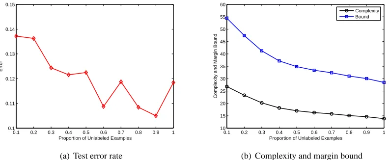
If we do not use iterative optimization, the empirical Rademacher complexity ˆRl(

G

)will involve

other two terms Θ and

J

. By a similar technique as in (32), we can show that Θonly depends on the unlabeled data and the kernel functions, while

J

encodes the interaction between labeled and unlabeled data. As a result, the margin bound relies on both labeled and unlabeled data. For this case, we will give an evaluation of the margin bound with different sizes of unlabeled sets in Section 6.4.

6. Experiments

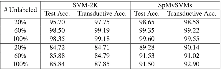
We performed experiments on artificial data and real-world data to evaluate the proposed sparse multi-view SVMs (SpMvSVMs). For SpMvSVMs withε>0, the entries of z were fixed as 1 for labeled data and initialized as 0.995 for unlabeled data. The termination condition for iterative optimization is either no unlabeled examples can be removed or the maximum iteration number sur-passes 50. Comparisons are made with supervised SVMs, and the unsupervised SVM-2K method. Each accuracy/error reported in this paper is an averaged accuracy/error value over ten random splits of data into labeled, unlabeled and test data.

−2 −1 0 1 2 3 −2

−1 0 1 2

Class 1 Class 2

(a) View 1

−2 −1 0 1 2

−1 0 1

2 Class 1

Class 2

(b) View 2

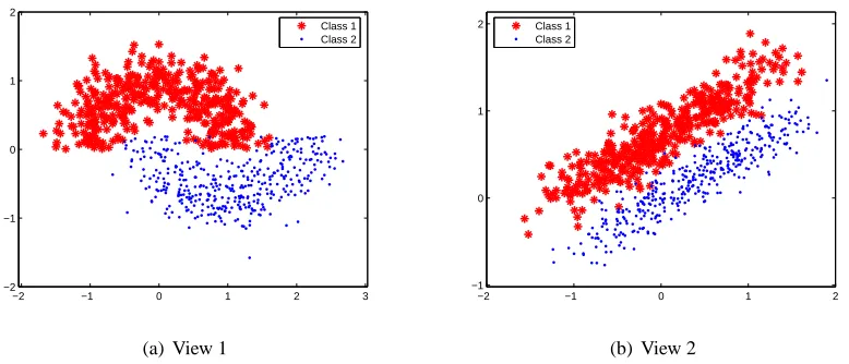
Figure 1: Examples in the two-moons-two-lines data set.

6.1 Artificial Data

This two-moons-two-lines synthetic data set was generated according to Sindhwani et al. (2005). Examples in two classes scatter like two moons in one view and two parallel lines in the other. To link the two views, points on one moon were enforced to associate at random with points on one line. Each class has 400 examples and a total of 800 examples were generated as shown in Figure 1. For SpMvSVMs, the numbers of examples in the labeled training set, unlabeled training set and test set were fixed as four, 596, and 200, respectively. Gaussian kernel with bandwidth 0.35 and the linear kernel were used for view 1 and view 2, respectively. The parameters γn and γv were

selected from a small grid_{10−6,10−4,10−2,1,10,100_}by five-fold cross validation on the whole data set. The chosen values areγn=10−4andγv=1. In this paper,γvis normalized by the number

of labeled and unlabeled examples involved in the multi-view regularization term. For supervised SVMs, which concatenated features from the two views, we also found the regularization coefficient from this grid by five-fold cross validation.

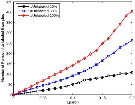
To evaluate SpMvSVMs, we varied the size of the unlabeled training set from 20%, 60% to 100% of the total number of unlabeled data, and used different values for the insensitive parameter

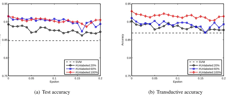
ε, which ranged from 0 to 0.2 with an interval 0.01 (when εis zero, sparsity is not considered). The test accuracies and transductive accuracies (on the corresponding unlabeled set) are given in Figure 2(a) and Figure 2(b), respectively. It should be noted that the numbers of data used to calculate transductive accuracies are different for the three curves in Figure 2(b). The numbers of removed unlabeled examples for differentεvalues are shown in Figure 3.

From Figure 2 and Figure 3, we find that with the increase of ε, more and more unlabeled data are removed, and the remove of a small number of unlabeled data can hardly decrease the performance of the resultant classifiers, especially when the original size of unlabeled set is large. Therefore, we can find a good balance between sparsity and accuracy using an appropriateε. In addition, more unlabeled data can benefit the performance of the learned classifiers with the same

0 0.05 0.1 0.15 0.2 0.8

0.85 0.9 0.95 1

Epsilon

Accuracy

SVM #Unlabeled:20% #Unlabeled:60% #Unlabeled:100%

(a) Test accuracy

0 0.05 0.1 0.15 0.2

0.8 0.85 0.9 0.95 1

Epsilon

Accuracy

SVM #Unlabeled:20% #Unlabeled:60% #Unlabeled:100%

(b) Transductive accuracy

Figure 2: Classification accuracies of SpMvSVMs with different sizes of unlabeled set andεvalues on the artificial data. The accuracies of SVMs are also shown.

0 0.05 0.1 0.15 0.2

0 50 100 150 200 250 300 350 400 450

Epsilon

Number of Removed Unlabeled Examples

#Unlabeled:20% #Unlabeled:60% #Unlabeled:100%

Figure 3: The numbers of unlabeled examples removed by SpMvSVMs for differentε values on the artificial data.

6.2 Text Classification

0 0.05 0.1 0.15 0.2 0.75

0.8 0.85 0.9 0.95

Epsilon

Accuracy

SVM #Unlabeled:20% #Unlabeled:60% #Unlabeled:100%

(a) Test accuracy

0 0.05 0.1 0.15 0.2

0.75 0.8 0.85 0.9 0.95

Epsilon

Accuracy

SVM #Unlabeled:20% #Unlabeled:60% #Unlabeled:100%

(b) Transductive accuracy

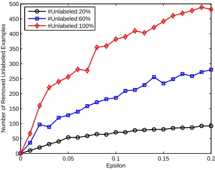
Figure 4: Classification accuracies of SpMvSVMs with different sizes of unlabeled set andεvalues on text classification. The accuracies of SVMs are also shown.

in all links pointing to the web page from other pages. We preprocessed each view by remov-ing stop words, punctuation and numbers and then applied Porter’s stemmremov-ing to the text (Porter, 1980). In addition, words that occur in five or fewer documents were ignored. This resulted in 2332 and 87-dimensional vectors in the first and second view, respectively. Finally, document vec-tors were normalized to t f.id f (the product of term frequency and inverse document frequency) features (Salton and Buckley, 1988).

For SpMvSVMs, the numbers of examples in the labeled training set, unlabeled training set and test set were fixed as 32, 699, and 320, respectively. In the training set and test set, the numbers of negative examples are three times of those of positive examples to reflect the overall proportion of positive and negative examples. The linear kernel was used for both views. The parametersγn

andγv for SpMvSVMs and the regularziation coefficient for SVMs were selected using the same

method as in Section 6.1. The chosen values for SpMvSVMs areγn=10−6andγv=0.01.

To evaluate SpMvSVMs, we also varied the size of the unlabeled training set from 20%, 60% to 100% of the total number of unlabeled data, and used different values for the insensitive parameter

εranging from 0 to 0.2 with an interval 0.01. The test accuracies and transductive accuracies are given in Figure 4(a) and Figure 4(b), respectively. The numbers of removed unlabeled examples for differentεvalues are shown in Figure 5.