Application of Non Parametric Empirical Bayes Estimation to High
Dimensional Classification
Eitan Greenshtein [email protected]
Central Bureau of Statistics 66 Kanfei Nesharim St Jerusalem, 95464, Israel
Junyong Park [email protected]
Department of Mathematics and Statistics University of Maryland Baltimore County Baltimore, MD 21250, USA
Editor: Bin Yu
Abstract
We consider the problem of classification using high dimensional features’ space. In a paper by Bickel and Levina (2004), it is recommended to use naive-Bayes classifiers, that is, to treat the features as if they are statistically independent.
Consider now a sparse setup, where only a few of the features are informative for classification. Fan and Fan (2008), suggested a variable selection and classification method, called FAIR. The FAIR method improves the design of naive-Bayes classifiers in sparse setups. The improvement is due to reducing the noise in estimating the features’ means. This reduction is since that only the means of a few selected variables should be estimated.
We also consider the design of naive Bayes classifiers. We show that a good alternative to variable selection is estimation of the means through a certain non parametric empirical Bayes pro-cedure. In sparse setups the empirical Bayes implicitly performs an efficient variable selection. It also adapts very well to non sparse setups, and has the advantage of making use of the infor-mation from many “weakly informative” variables, which variable selection type of classification procedures give up on using.
We compare our method with FAIR and other classification methods in simulation for sparse and non sparse setups, and in real data examples involving classification of normal versus malignant tissues based on microarray data.
Keywords: non parametric empirical Bayes, high dimension, classification
1. Introduction
We consider the problem of finding a classifier for a response variable Y∈ {−1,1}based on a vector
(X1, ...,Xp)∈Rpof explanatory variables.
Suppose we have a ‘training set’ (or a sample) of n1examples(Yi,Xi1, ...,Xip), i=1, ...,n1, for
which Yi=−1, and additional n2examples(Yi,Xi1, ...,Xip), i=n1+1, ...,n1+n2, for which Yi=1.
We assume that the n1+n2observations are independent. In what follows we assume for simplicity
that n1=n2≡n.
contemporary statistical applications where p≫n. We mention that of microarray data where the dimensionality is typically of thousands, while the sample size is of the order of dozens or hundreds.
In particular we focus on linear predictors for Y , which are of the form:
ˆ
Y =sign
p
∑
j=1ajXj+a0
!
,
where a0,a1, ...,apare constants.
Suppose the distribution of the explanatory variables, conditional on Y =−1 and on Y =1, is G1and G2correspondingly, where Giare multivariate normals i=1,2. Assume that the covariance
matrices of Gi, i=1,2 are the same. Then the optimal classifier is Fisher’s rule. However when the
common covariance matrix as well as the vectors of means under G1and G2are unknown, we can
not apply Fisher’s rule. When n≫p, the naive approach, of estimating the unknown quantities and plug-in to Fisher’s rule, would work well. It is impractical when p≫n . A practical solution, called ‘naive Bayes’ is to neglect estimation of the off diagonal elements in the covariance matrix (or to estimate them trivially) by setting those values to be 0. Then apply Fisher’s rule by plugging in the estimated diagonal covariance matrix and the estimated vectors of means. Bickel and Levina (2004) showed that in many cases, by this trivial estimation of the covariance matrix, one does not lose too much in terms of classification error, relative to incorporating the true covariance matrix, and suggested this practice. Note, the bottom line of this practice is to treat the explanatory variables as if they are independent, or act “assuming” independence of the explanatory variables. We will also refer in the sequel to Fisher’s rule as the Independence Rule, or IR.
It was pointed out independently by Fan and Fan (2008) and by Greenshtein et al. (2009), that even in the independent case, when p≫n, estimating the vector of means under G1and under G2by
the corresponding sample averages, could lead to a very weak estimator, resulting in a corresponding classifier with virtually no classification power (see Theorem 1 in Fan and Fan 2008, and Proposition 1 of Greenshtein et al. 2009). This is also in cases where there exists a good linear classifier. In other words, often, attempting to estimate the 2p coordinates of the two mean vectors, by the corresponding averages of n observations on each, is already “too much”, and leads to overfit. The FAIR approach suggested by Fan and Fan (2008), and the conditional MLE approach suggested by Greenshtein et al. (2009), are based on variable selection techniques followed by estimation of the mean of the selected explanatory variables, while ignoring the others (i.e., setting the corresponding coefficients of the linear classifier to be equal to zero). The FAIR method estimates the means of the selected variables by the corresponding sample means (the MLE), while the conditional MLE method estimates by the conditional MLE, conditional on the event that the variables were selected. The above approaches are helpful especially in a high dimensional sparse setup, while the non parametric Empirical Bayes approach that we will present is helpful also in non-sparse setups. Let
µ andτbe the vectors of means under G1and G2correspondingly; here ‘sparse’ setup means that
the vector
ν≡µ−τ
1.1 On Types of Sparsity
The term sparse vector is only loosely defined in the literature, and we will keep some of the am-biguity. However, by a sparse vector ν we mean that most of its coordinates are exactly zero. Throughout our study we consider only vectorsνsuch that their l2norm||ν||, is much smaller than
their dimension, say,||ν||=o(p). The last condition does not imply sparsity under our terminology. We concentrate on configurations such that||ν||=o(p), since that as p→∞, when letting||ν||=
O(p), any reasonable procedure would achieve asymptotically (virtually) zero misclassification rate. We are interested in the cases when there is not enough signal to make nearly perfect classification, that is, p≫ ||ν||. In our simulation, we achieve p≫ ||ν||, by considering the following three types of configurations for vectors||ν||:
(a) Very few non-zero coordinates of a large/moderate magnitude (i.e., sparse vectors)
(b) Very few coordinates of a large magnitude, mixed with many very small coordinates (i.e., non-sparse vectors).
(c) Many coordinates of a very small magnitude (i.e., non-sparse vectors).
In sparse configurations, our EB procedure is comparable to the other procedures. Specifically, it is better in moderately sparse setups, while in extremely sparse cases, it is inferior. Indeed, when there are only a few relevant variables, naturally methods which are based on variable selection would do well. In non-sparse configurations our EB procedure is clearly advantageous in simulations. This is in line with the theoretical results in Brown and Greenshtein (2009), and in Jiang and Zhang (2007), on optimality of non-parametric empirical Bayes in estimation of high dimensional not extremely sparse normal mean vectors, coupled with the relation between estimation and classification as explained in Section 2.
The above mentioned results, join a huge body of literature on Empirical Bayes starting with Robbins (1951), see the surveys by Copas (1969) and by Zhang (2003). See also a recent paper by Greenshtein and Rotov (2009) on efficiency of compound and empirical Bayes procedures with respect to the class of permutation invariant procedures. A recent comprehensive study and per-formance comparison, of various methods for estimating a vector of normal means under squared error loss, was conducted by Brown (2008), the very good performance of non parametric empiri-cal Bayes methods is demonstrated also there. Our approach is related to (and independent of) the approach in Efron (2009), where EB estimation method is used to obtain good classifiers.
We will introduce and explain the virtues of our empirical Bayes classification method and provide simulation evidence as well as real data evidence to its excellent performance. We will compare the performance of our Empirical Bayes classifiers to that of FAIR (Fan and Fan, 2008), conditional MLE (Greenshtein et al. , 2009), NSC (Tibshirani et al. , 2002), and plug in Fisher’s rule.
2. Preliminaries
Assume a multivariate normal distribution of the vector (X1, ...,Xp) conditional on the value of
Y . Specifically, we assume (Xj|Y =−1)∼N(µj,s2) and(Xj|Y =1)∼N(τj,s2) independently,
j=1, ...,p. We will assume that the variance s2is known. Denote µ= (µ1, ...,µp),τ= (τ1, ...,τp).
In considering linear classifiers, when both p and n are large it is robust to assume normality of
(X1, ...,Xp) by the central limit theorem. Due to Lindberg’s CLT, large p implies that∑ajXj will
be close to normal, when aj are comparable in size, even if the individual Xj are not normal. In
addition, large n implies that averages of independent Xi j, i=1, ...,n (as in Zj, which is defined
in the sequel) are close to normal. The CLT arguments are problematic when the Xjs have heavy
tails. In Table 5 of Section 4 some simulations are carried to demonstrate the effect of heavy tailed distributions.
When searching for values a≡(a1, ...,ap)that determine a ‘good’ linear classifier, we assume
w.l.o.g. that kak2=∑pj=1a2j =1. In this case the optimal choice of(a1, ...,ap) is the vector that
maximizes|∑ajµj−∑ajτj|. Note that the optimal choice of a1, ...,ap is the same regardless of
the misclassification loss (the value of a0does depend on the loss). In order to see it, observe that
∑ajXj ∼N(∑ajµj,s2)≡N(θ1,s2)conditional on Y=−1 and∑ajXj∼N(∑ajτj,s2)≡N(θ2,s2)
conditional on Y =1; hereθi,=1,2 are implicitly defined. Hence, an optimal choice of a1, ...apis
such that
V =V(a1, ...,an)≡ |
∑
jajµj−
∑
jajτj|=|θ1−θ2| (1)
is maximized. This implies that the coordinates aoptj of the optimal choice satisfy:
aoptj = qνj
∑ν2 j
, j=1, ...p; (2)
recallνj=µj−τj.
Under a 0-1 loss, given any choice of(a1, ...,ap), the corresponding minmax choice of a0is
a0=−
θ2+θ1
2 .
This is also the Bayes solution assuming a priorπi=0.5 for each class. The optimal choice of a0
for none-equal losses and priors is straightforward.
A formal argument showing that the optimal a1, ...,ap is the same regardless of the
misclas-sification loss may be obtained using the theory of comparison of experiments, implying that the experiment that consists of the distributions N(θ1,s2)and N(θ2,s2), dominates the experiment that
consists of the distributions N(θ′1,s2)and N(θ′2,s2)if and only if|θ1−θ2| ≥ |θ′1−θ′2|. See Lehmann
(1986, p. 86), for some basic theory on comparison of experiments and some additional references. By the above discussion there is a natural order relationbetween two classifiers determined by a and a′. We say that aa′if for the correspondingθiandθ′i,
V =|θ′1−θ′2| ≥ |θ1−θ2|=V′ (3)
Note, here V ≡V(a1, ...,ap), is a function of(a1, ...,ap).
By (2), V(aopt1 , ...,aoptp ) =||ν||, consequently for the optimal choice aopt0 , the Bayes risk is:
Φ(−||ν||
2s ) (4)
2.1 Summary
The goal of finding the optimal classifier whenνj, j=1, ...,p are unknown, is not practical.
How-ever we want to find a classifier with a corresponding ‘large’ value of V.
Note, in statistical inference the choice of aj, j=1, ...,p depends on the data. The dependence
on the data is through the vector
Z= (Z1, ...,Zp); here, for n=n1=n2
Zj=∑
n i=1Xi j
n −
∑2n i=n+1Xi j
n , j=1, ...,p, (5)
are independent normal random variables with EZj=νjand variance, denotedσ2,
σ2=2s2
n . (6)
Thus, depending on the particular procedure the selected value of ajdepends on Z1, ...,Zp, and
it is a random variable denoted ˆaj, j=1, ...,p.
Equation (3), motivates us to search for procedures with high value of
E(V) =E|
p
∑
j=1ˆ ajνj|.
Thus we extend the definition of the order relation, to apply to two statistical procedures{aˆj}, j=
1, ...,p,and{aˆ′j}, j=1, ...,p.
Definition 1: We say that{aˆ′j}, j=1, ...,p,dominates{aˆj}, j=1, ...,p,if for the
correspond-ing V′and V , E(V′)≥E(V).
Remark 1: Evaluating a procedure ˆaj j=1, ...,p, by its corresponding value E(V), is simplistic,
for example, it ignores the effect of the standard deviation of V on the classification error. However, in high dimensional setup one might hope that the standard deviation of V is small compare to E(V). Otherwise, one might perceive it as a convenient approximate evaluation. Note however, that for two procedures with very accurate classification rate, ignoring the variability of V might be significantly misleading even if E(V)is large compare to the standard deviation of V , this is due to the thin tail of the normal distribution.
2.2 On the Relation Between Estimating the Mean Under a Squared Loss and Classification
Since the optimal choice of aj, j=1, ...,p, is aoptj =
νj
q
∑ν2
j
,a natural way to proceed is to estimate
νj by a ‘good’ estimator ˆνj forνj, and then plug-in, that is, let ˆaj= ˆ
νj
q
∑νˆ2
j
.A formal definition of
‘good’ in the above, depends on the loss function. In the sequel we will indicate why the squared error loss function is especially appropriate.
First we state the obvious. In general, the fact that ˆνis a good estimator forνunder a squared error loss, does not indicate that T(νˆ)is a good estimator for T(ν)under (say) a squared loss. For example in the case T(ν) =∑νj, plugging in the MLE forνwill often be better than plugging in
do not automatically indicate that it should be plugged-in in order to obtain good estimators for aoptj , and thus provide good classifiers.
Consider the collection of all vectors(a1, ...,ap)with l2norm 1. Define the function
L((a1, ...,ap)) =
∑
(νj−aj)2Then, one may check that on the surface of the p dimensional unit ball,
L(a) =−2×V(a) +C,
where C=1+∑ν2
j, and V is defined in (1).
The last equation motivates the particular choice of a squared error loss when evaluating an estimator ˆνj. This is because of the direct relation between minimizing E(L)to that of maximizing
E(V). Maximizing V is crucial in obtaining a good classifier, as explained in the first part of this section.
An estimator with particularly appealing properties, in estimation of a vector of means under a squared loss in high dimensions, is the non-parametric empirical Bayes estimator, see Brown and Greenshtein (2009). We describe it in the following section and then define our procedure.
For a givenνthe success in obtaining a good classifier has to do with two aspects. The larger is the l2norm ofνthe smaller is the misclassification rate of the Bayes procedure, as may be seen in
(4), and typically also the misclassification rate of our EB procedure. The more difficult is the task of estimatingνby our non parametric empirical Bayes method in terms of MSE, the less successful is our classification method. As pointed by a referee, the difficulty/MSE in estimatingνby EB is invariant under translation, while (obviously) the l2 norm is not. When the vectorνis identically
zero (i.e., no signal) the corresponding misclassification rate is 0.5. The corresponding rates for various translations of the zero-vector may be found in Table 4.
3. Empirical Bayes Classification
In this section, we define our linear classifier for the cases of known homoscedastic variances and unknown heteroscedastic variances.
3.1 Known Homoscedastic Variance
In the sequel we rescale Xj, so that Zj defined in (5) will have varianceσ2=1, j=1, ...,p. This
is possible since s, the common standard deviation of Xj, is known see (6). When the variances are
unknown (and not assumed equal) we simply standardize the variables using the sample variance. The extension of this subsection for the latter case and for non equal samples n1and n2is explicitly
given in the next subsection.
Under the non-parametric empirical Bayes approach for estimating a vector of means, we con-sider the means νi =E(Zi), i=1, ...,p, as realizations of i.i.d random variables M1, ...,Mp
dis-tributed G, where G is completely unknown. Still, we attempt to approximate the Bayes estimator of the mean, denotedδG(z), by ˆδ(z). Then we estimateνiby ˆνi=δˆ(Zi).
More formally it is described in the following. Let Z∼N(M,1)where M∼G, G∈
G
. We want to emulate the Bayes procedureδGbased on a sample Z1, ...,Zp, Zi∼N(Mi,1), i=1, ...,p, whereLet g∗be the mixture density
g∗(z) =
Z
φ(z−ν)dG(ν).
Then from Brown (1971) equation (1.2.2), we have that the Bayes procedure, denotedδG,
sat-isfies
δG(z) =z+g∗
′
(z)
g∗(z);
here g∗′(z)is the derivative of g∗(z). The estimator that we suggest forδG, is of the form
ˆ
δh(z) =z+
ˆ g∗h′(z)
ˆ g∗h(z)
where ˆg∗h′(z) and ˆg∗h(z) are appropriate kernel estimators for the density g∗(z) and its derivative g∗′(z). The subscript h denotes the bandwidth of the kernel estimator. We will use a normal kernel.
Let h>0 be a bandwidth constant. Then define the kernel estimator
ˆ
g∗h(z) = 1
nh
∑
φ(z−Zi
h ).
Its derivative is:
ˆ
g∗h′(z) = 1
nh
∑
Zi−z
h ×φ(
z−Zi
h ).
In Brown and Greenshtein (2009), it is suggested to let the bandwidth converge slowly to zero as p→∞, they suggested that h2should approach zero ‘just faster’ than 1/log(p). In the simulations and real data analysis in this paper, we applied h=0.3≈1/p
log(p), which is in agreement with that suggestion for the range of features’ dimensions p that we study. The choice h=1/p
log(p)is also suggested in Brown and Greenshtein (2009) as a ‘default’ choice. A more careful choice could involve, for example, cross validation. However, the results are not too sensitive to the choice.
3.2 The Empirical Bayes Classifier
We now define our Empirical Bayes classifier. Let
ˆ
νi=δˆh(Zi), i=1, ...,p.
Let
ˆ ai=
ˆ νi
q
∑jνˆ2j
i=1, ...,p.
In order to fully define our classifier, we should still define the parameter ˆa0, given ˆa1, ...,aˆp.
We do it for the case of 0-1 loss and equal prior probabilities for each class. An obvious way is the following. Let ˆθ1=1n∑ni=1∑
p
j=1aˆjXi j, where the summation is over the n examples(Yi,Xi1, ...,Xip)
for which Yi=−1. Similarly define ˆθ2.
Let,
ˆ
a0=−
ˆ θ2+θˆ1
2 .
3.3 Unknown Heteroscedastic Variances
Consider now the case where the standard deviation, denoted sj, of Xj are unknown j=1, ...,p.
We now introduce a superscript k=1,2 to denote quantities associated with the data corresponding to Y =−1 and Y =1. Denote by ˆskj the usual estimates of the standard deviation of Xjk. The estimates are based on the corresponding Xi jk, k=1,2, i=1, ...,nk, j=1, ...,p. Denote ¯X1j and ¯X2j
the corresponding means. Let
ˆ Sj=
s
(sˆ1 j)2
n1 +(sˆ
2 j)2
n2 ,
thus ˆSjis our estimator for the standard deviation of ¯X1j −X¯2j.
Let
Zj=
¯ X1j −X¯j2
ˆ Sj
;
note, we expect that the variance of Zjis approximately 1, j=1, ...,p.
As before let ˆνibe the empirical Bayes estimators of E(Zi), and let ˆai=qνˆi
∑jνˆ2j
, i=1, ...,p.
In the following we proceed in terms of the variables
Uj=
Xj
ˆ Sj
j=1, ...,p.
We will represent our linear classifiers as linear functions of Uj, j=1, ...,p.
Let
ˆ θk=
1 nk
nk
∑
i=1p
∑
j=1ˆ
ajUi jk,k=1,2.
Let
ˆ
a0=−
ˆ θ2+θˆ1
2 .
Finally, our classifier is:
sign( p
∑
j=1ˆ
ajUj+aˆ0).
4. Simulations and Data Analysis
In this section, we present numerical studies including simulations and application to three sets of real data.
4.1 Simulations
The simulation study in this subsection is based on the procedure described in Section 3.1. We present simulations for p=105and for p=104, under various configurations in whichτj=0, j=
1, ...,p. We study sparse configurations where for l variables the corresponding mean is fixedνj=∆,
while the remaining p−l variables have νj =0, p≫l. We also study a non-sparse version of
N(0,0.12). The small variance of the normal distribution is in order to control the magnitude of
||ν||; recall from the introduction, we want p≫ ||ν||. Thus a configuration is determined by(∆,l), the corresponding p, and whether the p−l coordinates, whose means are not equal to∆, are set to be equal to zero or, alternatively get their values randomly based on a N(0,0.12)distribution.
We consider the case where n=25, and a rescale under which the variance of Zj is σ2 =1,
j=1, ...,p. Thus, the variance of Xj is s2=25/2, and the same for the variance of∑ajXj, when
∑a2j =1. The distribution Xjis normal throughout this section, except for the simulations reported
in Table 5. In Table 5 the effect of a heavy tailed distribution variables Xjis studied.
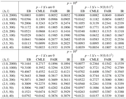
Table 1 shows the misclassification rates of the empirical Bayes, conditional MLE, FAIR, and the plug in Fisher’s rule which is also termed IR (Independence Rule). The plug in Fisher’s refers to plugging in Zj forνj, j=1, ...,p, in Fisher’s rule. We see that the empirical Bayes approach
produces the best results for non-sparse and for moderately sparse configurations. The CMLE is better for strongly sparse configurations. The version of FAIR we are using is described in Theorem 4 of Fan and Fan (2008). It performs similar to IR, since it selects too many variables. Fan and Fan (2008) describe another version of FAIR in their equation (4.3), this other version screens variables more aggressively and involves computation of eigenvalues of the empirical covariance matrix. That more aggressive version might perform better in our simulation, yet it is motivated for cases where it is not known that the covariance matrix is of the formσ2I (which is used in most of our simulations). In addition, computing eigenvalues for empirical covariance matrix with p=105is computationally intensive. In the real data analysis, with unknown covariance matrix, the other version of FAIR is used.
Each entry is based on simulated Z1, ...,Zp, and on calculating the exact theoretical
misclassifi-cation rate. Note, given the estimators ˆaj j=0,1, ...,p, for a given simulated realization, the
the-oretical misclassification error, under equal prior probability for each class, is 12Φ((−∑pj=1aˆjµj−
ˆ
a0)/s) +12(1−Φ((−∑pj=1aˆjτj−aˆ0))/s).
In order to demonstrate the effect of dependence and to compare the methods for correlated vari-ables, we also consider correlated normal variables where the correlation of Xiand Xj, namelyρi j,
has the form ofρ|i−j| known as AR(1) model. Here, the corresponding misclassification probabili-ties are 12Φ((−∑pj=1aˆjµj−aˆ0)/
√
ˆa′S ˆa) +12(1−Φ((−∑pj=1aˆjτj−aˆ0))/
√
ˆa′S ˆa), for the appropriate
covariance matrix S.
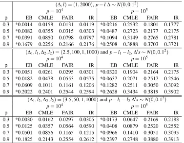
Table 2 presents misclassification rates under different values of ρ. The empirical Bayes still achieves the lowest error rates for all those non-sparse configurations. The reported entries are averages of the 100 error rates corresponding to 100 realizations and corresponding estimators ˆaj
for the particular configuration (∆,l) or (∆1,l1,∆2,l2) where (∆1,l1,∆2,l2) means that l1 and l2
coordinates inνare all valued∆1and∆2correspondingly, while the remaining entries are all zero.
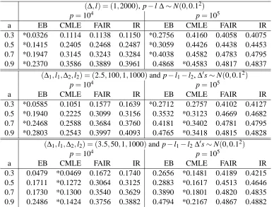
In Table 3 we present simulation results under the following correlation structure which is much heavier than that of AR(1). We consider correlations corr(Xi,Xj) =ρi j =αiαj for i6= j which is
easily implemented by letting Xi=τi(or µi) +
q
1−α2iWi+αiU where Wi’s 1≤i≤p and U are
generated independently from N(0,s2). In our simulations, all α′is are generated from U(−a,a)
where a=0.3,0.5, 0.7 and 0.9 are considered. As a increases, variables are more correlated. Table 3 shows misclassification probabilities for configurations of(∆,l)or(∆1,l1,∆2,l2)as in Table 2.
p=104
p−l∆’s are 0 p−l∆’s∼N(0,0.12)
(∆,l) EB CMLE FAIR IR EB CMLE FAIR IR
(1.0, 2000) *0.0003 0.0091 0.0052 0.0052 *0.0000 0.0082 0.0049 0.0049
(1.0, 1000) *0.0396 0.1309 0.0906 0.0905 *0.0162 0.1182 0.0854 0.0852
(1.0, 500) *0.2006 0.3243 0.2475 0.2474 *0.1055 0.3139 0.2341 0.2339
(1.5, 300) *0.1172 0.1891 0.1805 0.1806 *0.0657 0.1771 0.1679 0.1680
(2.0, 200) *0.0521 0.0868 0.1413 0.1416 *0.0340 0.0813 0.1315 0.1318
(2.5, 100) *0.0529 0.0631 0.1985 0.1990 *0.0396 0.0632 0.1863 0.1867
(3.0, 50) 0.0641 *0.0604 0.2677 0.2682 *0.0518 0.0583 0.2532 0.2536
(3.5, 50) 0.0113 *0.0099 0.2019 0.2025 *0.0093 0.0095 0.1893 0.1898
(4.0, 40) 0.0042 *0.0033 0.1933 0.1939 0.0039 *0.0034 0.1807 0.1812
p=105
p−l∆’s are 0 p−l∆’s∼N(0,0.12)
(∆,l) EB CMLE FAIR IR EB CMLE FAIR IR
(1.0, 2000) *0.1444 0.2717 0.1896 0.1894 *0.0077 0.2364 0.1542 0.1539
(1.0, 1000) *0.3100 0.3952 0.3294 0.3293 *0.0367 0.3721 0.2792 0.2789
(1.0, 500) *0.4067 0.4552 0.4122 0.4121 *0.0702 0.4408 0.3567 0.3565
(1.5, 300) *0.3643 0.3868 0.3817 0.3818 *0.0628 0.3744 0.3278 0.3278
(2.0, 200) *0.3071 0.2865 0.3609 0.3611 *0.0522 0.2727 0.3080 0.3081
(2.5, 100) 0.3009 *0.2275 0.3901 0.3903 *0.0560 0.2261 0.3358 0.3359
(3.0, 50) 0.3006 *0.1887 0.4202 0.4204 *0.0597 0.1886 0.3649 0.3649
(3.5, 50) 0.1521 *0.0474 0.3927 0.3929 *0.0263 0.0507 0.3387 0.3388
(4.0, 40) 0.0792 *0.0162 0.3876 0.3879 *0.0121 0.0157 0.3339 0.3340
Table 1: Misclassification error rates by Empirical Bayes, conditional MLE (Greenshtein et al. 2009), FAIR (Fan and Fan 2008) and Fisher’s rule (i.e., without variable selection)) . Error rate with * represents minimum error rate in the row for the corresponding configuration.
variables, so more correlations are in effect, relative to variable selection methods that screen vari-ables and consequently their correlations do not effect.
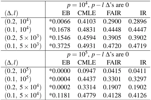
In Table 4, we compare the above mentioned procedures in non sparse setups where there are many small signals. In all the configurations there is ’enough overall signal’ to make virtually no classification error if µ and τwere known. In those configurations the optimal (unknown) linear classifiers uses most (or all) of the variables. However, attempting to estimate the corresponding means by FAIR or Fisher’s plug-in and the Conditional MLE methods yield poor classifiers, while the non parametric empirical Bayes method yields classifiers with excellent performance in some cases.
In Table 5, we present simulation studies for Xjs with a heavy tailed distribution. As before
n1=n2=25. Under G1 the distribution of Xj is c×t(3) (i.e., t with 3 degrees of freedom), j=
1, ...,p where c is chosen so that the variance of Xjis s2=25/2. Under G2the distribution of Xjis
νj+c×Xj, where Xjis distributed t(3), j=1, ...,p. Thus, the corresponding Zj has variance 1 and
it is only approximately normal. We study the configurations(∆,l) = (1,2000),(2.5,100),(3.5,50)
(∆,l) = (1,2000), p−l∆∼N(0,0.12)
p=104 p=105
ρ EB CMLE FAIR IR EB CMLE FAIR IR
0.3 *0.0014 0.0158 0.0131 0.0119 *0.0216 0.2532 0.1801 0.1777
0.5 *0.0082 0.0355 0.0315 0.0303 *0.0487 0.2723 0.2177 0.2175
0.7 *0.0391 0.0850 0.0798 0.0797 *0.1094 0.3149 0.2765 0.2781
0.9 *0.1679 0.2256 0.2166 0.2176 *0.2508 0.3888 0.3703 0.3721
(∆1,l1,∆2,l2) = (2.5,100,1,1000)and p−l1−l2,∆′s∼N(0,0.12)
p=104 p=105
ρ EB CMLE FAIR IR EB CMLE FAIR IR
0.3 *0.0051 0.0261 0.0295 0.0301 *0.0320 0.1904 0.2164 0.2175
0.5 *0.0182 0.0478 0.0553 0.0575 *0.0637 0.2071 0.2517 0.2546
0.7 *0.0609 0.1011 0.1161 0.1206 *0.1282 0.2511 0.3050 0.3092
0.9 *0.2022 0.2401 0.2544 0.2594 *0.2628 0.3434 0.3819 0.3902
(∆1,l2,∆2,l2) = (3.5,50,1,1000)and p−l1−l2∆′s∼N(0,0.12)
p=104 p=105
ρ EB CMLE FAIR IR EB CMLE FAIR IR
0.3 *0.0030 0.0162 0.0297 0.0305 *0.0173 0.0647 0.2169 0.2183
0.5 *0.0125 0.0357 0.0564 0.0590 *0.0408 0.0879 0.2520 0.2552
0.7 *0.0501 0.0856 0.1165 0.1215 *0.0966 0.1410 0.3051 0.3095
0.9 *0.1825 0.2143 0.2554 0.2612 *0.2397 0.2748 0.3880 0.3913
Table 2: Dependent case I : Corr(Xi,Xj) =ρi j =ρ|i−j| for ρ=0.3,0.5 and 0.7. (∆1,l1,∆2,l2)
represents l1and l2coordinates inνare∆1and∆2respectively.
produce smaller error rates compared to FAIR and IR. However, compared to the results in Table 1, the EB method and CMLE have a worst performance which is caused by some sensitivity to the heavy tailed distribution of the Xjs.
Summary: The most important advantage of the EB classifier, demonstrated in the above
simula-tions, is its ability to use the information provided by many small signals in order to improve the classification. This is unlike variable-selection type of classifiers, that give up on using the informa-tion from variables with smallνj, in order to reduce the variability in estimation. This advantage is
not on the expanse of being a good classifier also under moderately sparse configurations.
4.2 Real Data Analysis
The following analysis of real date sets is based on the procedure described in Section 3.2. We con-sider three real data sets and compare the empirical Bayes approach with nearest centroid shrunken (henceforth NSC), and FAIR. The NSC was proposed by Tibshirani et al. (2002). The three data sets were studied by Fan and Fan (2008), and all the misclassification rates, other than that of the empirical Bayes method, are cited from that paper.
(∆,l) = (1,2000), p−l∆∼N(0,0.12)
p=104 p=105
a EB CMLE FAIR IR EB CMLE FAIR IR
0.3 *0.0326 0.1114 0.1138 0.1150 *0.2756 0.4160 0.4058 0.4075
0.5 *0.1415 0.2405 0.2468 0.2487 *0.3059 0.4426 0.4438 0.4453
0.7 *0.1947 0.3145 0.3243 0.3284 *0.4038 0.4582 0.4783 0.4795
0.9 *0.2370 0.3586 0.3889 0.3961 0.4868 *0.4583 0.4817 0.4837
(∆1,l1,∆2,l2) = (2.5,100,1,1000)and p−l1−l2,∆′s∼N(0,0.12)
p=104 p=105
a EB CMLE FAIR IR EB CMLE FAIR IR
0.3 *0.0585 0.1051 0.1577 0.1639 *0.2712 0.2757 0.4102 0.4127
0.5 *0.1940 0.2225 0.3099 0.3156 0.3532 *0.3123 0.4669 0.4682
0.7 *0.2468 0.2588 0.3684 0.3760 0.4181 *0.3402 0.4781 0.4795
0.9 *0.2803 0.2543 0.3997 0.4093 0.4765 *0.3418 0.4815 0.4828
(∆1,l1,∆2,l2) = (3.5,50,1,1000)and p−l1−l2∆′s∼N(0,0.12)
p=104 p=105
a EB CMLE FAIR IR EB CMLE FAIR IR
0.3 0.0479 *0.0469 0.1672 0.1740 0.2656 *0.1481 0.4189 0.4215
0.5 0.1711 *0.1272 0.3064 0.3125 0.2883 *0.1617 0.4513 0.4646
0.7 0.1730 *0.1300 0.3540 0.3629 0.3890 *0.1801 0.4820 0.4835
0.9 0.2486 *0.1424 0.3756 0.3882 0.4794 *0.2167 0.4867 0.4882
Table 3: Dependent case II : Corr(Xi,Xj) =ρi j=αiαjfor i6=j whereαiandαjare generated from
U ni f(−a,a)for a=0.3,0.5, 0.7 and 0.9. (∆1,l1,∆2,l2)represents l1and l2coordinates in
νare∆1and∆2respectively.
set has 38 ( n1=27 in ALL and n2=11 in AML) and the test data set has 34 (20 in ALL and 14
in AML). Table 6 shows the results of the nearest shrunken centroid, FAIR, and empirical Bayes methods.
The empirical Bayes approach misclassified 3 out of 34 test samples which is the same result as NSC, but slightly worse than FAIR. Figure 1 shows histograms of∑jaˆjUjcorresponding to the two
groups, under the training and under the test sets.
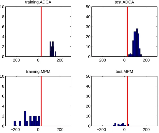
The second example is of lung cancer data which were previously analyzed by Gordon et al. (2002) and analyzed using FAIR in Fan and Fan (2008). The data is available at http: //www.chestsurg.org. There are p=12533 genes and 181 samples coming from two classes, MPM(malignant pleural mesothelioma) and ADCA(adenocarcinoma). The training sample set con-sists of 32 samples(n1=16 from MPM and n2=16 from ADCA) and the test has 149 samples (15
from MPM and 134 from ADCA). As displayed in Table 7, the empirical Bayes method classified all the training samples correctly and 148 out of 149 test samples correctly, which is a significant improvement compared to NSC and FAIR. In Figure 2, we show histograms of ∑aˆjUj under the
two groups, for the training and for the test sets.
p=104, p−l∆’s are 0
(∆,l) EB CMLE FAIR IR
(0.2,104) *0.0066 0.4103 0.2900 0.2896
(0.1,104) *0.1678 0.4831 0.4448 0.4447
(0.2,5×103) *0.1546 0.4594 0.3905 0.3902
(0.1,5×103) *0.3725 0.4931 0.4720 0.4719 p=105, p−l∆’s are 0
(∆,l) EB CMLE FAIR IR
(0.2,105) *0.0000 0.0947 0.0415 0.0411
(0.1,105) *0.0004 0.4437 0.3301 0.3297
(0.2,5×104) *0.0002 0.3314 0.1907 0.1902
(0.1,5×104) *0.1181 0.4779 0.4128 0.4126 Table 4: Non-sparse case
p=104
p−l∆’s are 0 p−l∆’s∼N(0,0.12)
(∆,l) EB CMLE FAIR IR EB CMLE FAIR IR
(1.0, 2000) 0.0350 0.1855 0.0152 *0.0149 0.0267 0.2126 0.0084 *0.0081
(2.5, 100) 0.1888 *0.1639 0.2121 0.2123 *0.1576 0.1600 0.1959 0.1969
(3.5, 50) 0.0994 *0.0791 0.2111 0.2112 0.2045 *0.1967 0.2643 0.2650
(4.0,40) 0.0744 *0.0640 0.2050 0.2055 0.0714 *0.0681 0.1933 0.1939
p=105
p−l∆’s are 0 p−l∆’s∼N(0,0.12)
(∆,l) EB CMLE FAIR IR EB CMLE FAIR IR
(1.0, 2000) 0.4331 0.4385 0.2179 *0.2170 0.2667 0.4325 *0.1886 0.1897
(2.5, 100) 0.4335 0.4155 *0.4018 0.4018 *0.3115 0.3926 0.3518 0.3517
(3.5, 50) 0.3661 *0.3365 0.4027 0.4023 *0.2966 0.3560 0.3562 0.3562
(4.0,40) 0.3528 *0.3282 0.4017 0.4023 *0.2815 0.3202 0.3544 0.3542
Table 5: Heavy tail case.
Method Training error Test error
Nearest shrunken centroids 1/38 3/34
FAIR 1/38 1/34
E.B. 0/38 3/34
Table 6: Classification errors of Leukemia data set
Method Training error Test error
Nearest shrunken centroids 0/32 11/149
FAIR 0/32 7/149
E.B. 0/32 1/149
−200 −1000 0 100 200 300 2
4 6 8 10
training, ALL
−200 −1000 0 100 200 300 2
4 6 8 10
test, ALL
−200 −1000 0 100 200 300 2
4 6 8 10
training, AML
−200 −1000 0 100 200 300 2
4 6 8 10
test, AML
Figure 1: Histograms of∑jaˆjUjof ALL and AML for training and test sets of Leukemia data. Two
panels in the first columns are histograms for ALL and AML from training sets and two in the second columns are for ALL and AML from test sets. Red vertical lines in all histograms represent cut off value which is−aˆ0= (θˆALL+θˆAML)/2=−15.10
−200 0 200
0 2 4 6 8 10
training,ADCA
−200 0 200
0 10 20 30 40 50
test,ADCA
−200 0 200
0 2 4 6 8 10
training,MPM
−200 0 200
0 10 20 30 40 50
test,MPM
Figure 2: Histograms of∑jaˆjUj of ADCA and MPM for training and test sets of lung cancer data.
Method Training error Test error
Nearest shrunken centroids 8/102 9/34
FAIR 10/102 9/34
E.B. 38/102 4/34
Table 8: Classification errors of Prostate Cancer data set
−5000 0 500 1000 1500 5
10 15 20
training, normal
−1500 −1000 −5000 0 500 1000 5
10 15 20
test, normal
−5000 0 500 1000 1500 5
10 15 20
training, tumor
−1500 −1000 −5000 0 500 1000 5
10 15 20
test, tumor
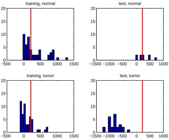
Figure 3: Histograms of∑jaˆjUj of normal and tumor for training and test sets of prostate cancer
data. Two panels in the first columns are histograms for normal and tumor from training sets and two in the second columns are for normal and tumor from test sets. Red verti-cal lines in all histograms represent cut off value which is−a0= (θˆnormal+θˆtumor)/2=
213.68.
independent test data set, from a different experiment, has 25 tumor and 9 normal samples. There are p=12600 genes.
As displayed in Table 8, for the prostate cancer data, the empirical Bayes approach has a very large training error compared to NSC and FAIR, but the test error is smaller than both NSC and FAIR. The pessimism of the misclassification error, reflected by our training set, may be attributed to two facts. One is the difference in the proportion of tumor and normal samples in the training versus the test set. The other reason is that the test set seems to be less noisy. It seems that the empirical Bayes method succeed in estimatingνjand hence deriving good coefficients ˆaj from the
large training data although it is noisy; yet, the classification of the individual data points of the noisy training set is still difficult, while the classification is easier for the test set data points. Figure 3 might be helpful in assessing it. In the histograms of∑jaˆjUj corresponding to the normal and
−0.080 −0.06 −0.04 −0.02 0 0.02 0.04 0.06 0.08 200
400 600 800 1000 1200
a
−0.080 −0.06 −0.04 −0.02 0 0.02 0.04 0.06 0.08 500
1000 1500 2000 2500
a
−0.060 −0.05−0.04−0.03−0.02−0.01 0 0.01 0.02 0.03 0.04 500
1000 1500 2000 2500 3000
a
Figure 4: Histograms of ˆaj, j=1, ...,p, for the leukemia, lung cancer, and prostate cancer data sets.
0.04 0.045 0.05 0.055 0.06 0.065 0.07 0.075 0.08 0
5 10 15 20 25
0.02 0.03 0.04 0.05 0.06 0.07 0.08 0
1 2 3 4 5 6 7 8 9
0.02 0.025 0.03 0.035 0.04 0.045 0.05 0.055 0.06 0
1 2 3 4 5 6 7 8 9
Figure 5: Histograms of the first 50 largest|aˆj|for the leukemia, lung cancer, and prostate cancer
data sets.
4.3 Number of Selected Variables
Figure 4 shows the histograms of ˆaj, j=1, ...,p for each data set. In Figure 5 we see three
his-tograms corresponding to the fifty largest |aˆj|, j=1, ...,p,in each of the three data sets. Our
empirical Bayes method uses many variables for the classification. In fact, formally it uses all the variables, since none of the ˆaj is exactly 0. In comparison the FAIR uses 11, 31, and 2 variables
corresponding to the above three cases in the order they presented, while the NSC uses 21, 26, 6. Obviously a method which is based on a few variables is easy to implement and to interpret. Our suggested classifiers are meant only to produce good classification and thus use many variables if necessary. Using many variables and somewhat complicated classifiers is in the spirit of data mining approach. However, selecting a subset of variables following an empirical Bayes estimation of the means, makes much sense, for producing simpler classifiers. It might even reduce noise and will produce over all better classifiers.
Acknowledgments
References
P.J. Bickel and E. Levina. Some theory for Fisher’s linear discriminant function, ”naive Bayes”, and some alternatives where there are many more variables than observations. Bernoulli, 10(6):989-1010, 2004.
L.D. Brown. Admissible estimators, recurrent diffusions, and insoluble boundary value problems. The Annals of Mathematical Statistics, 42(3):855-903, 1971.
L.D. Brown. In-season prediction of batting averages: a field-test of simple empirical Bayes and Bayes methodologies. Annals of Applied Statistics, 2(1):113-152, 2008.
L.D. Brown and E. Greenshtein. Nonparametric empirical Bayes and compound decision ap-proaches to estimation of a high-dimensional vector of means. Annals of Statistics, 37(4):1685-1704, 2009.
J.B. Copas. Compound decisions and empirical Bayes. Journal of the Royal Statistical Society Se-ries B(Methodological), 31(3):397-425, 1969.
B. Efron. Empirical Bayes estimates for large-scale prediction problems. Journal of the American Statistical Association, forthcoming.
J. Fan and Y. Fan. High dimensional classification using features annealed independence rules. Annals of Statistics, 36(6):2605-2637, 2008.
E. Greenshtein, J. Park, and G. Lebannon. Regularization through variable selection and conditional mle with application to classification in high dimensions. Journal of Statistical Planning and Inference, 139(2):385-395, 2009.
E. Greenshtein and Y. Ritov. Asymptotic efficiency of simple decisions for the compound decision problem. The Third Lehmann Symposium, IMS Lecture Notes Monograph Series, forthcoming.
T.R. Golub, D.K. Slonim, P. Tamayo, C. Huard, M. Gaasenbeek, J.P. Mesirov, H. Coller, M.L. Loh, J.R. Downing, M.A. Caligiuri, C.D. Bloomfield, and E.S. Lander. Molecular classification of cancer: class discovery and class prediction by gene expression monitoring. Science, 286:531-537, 1999.
G.J. Gordon, R.V. Jensen, L.L. Hsiao, S.R. Gullans, J.E. Blumenstock, S. Ramaswamy, W.G. Richards, D.J. Sugarbaker, and R. Bueno. Translation of microarray data into clinically relevant cancer diagnostic tests using gene expression ratios in lung cancer and mesothelioma. Cancer Res, 62(17):4963-4967, 2002.
W. Jiang and C.H. Zhang. General maximum likelihood empirical Bayes estimation of normal means. Annals of Statistics, 37(4):1647-1684, 2009.
E.L. Lehmann. Testing Statistical Hypothesis. Wiley, 1986.
D. Singh, P.G. Febbo, K. Ross, D.G. Jackson, J. Manola, C. Ladd, P. Tamayo, A.A. Renshaw, A.V. D’Amico, J.P. Richie, E.S. Lander, M. Loda, P.W. Kantoff, T.R. Golub, W.R. Sellers. Gene expression correlates of clinical prostate cancer behavior. Cancer Cell, 1(2):203-209, 2002.
R. Tibshirani, T. Hastie, B. Narasimhan, and G. Chu. Diagnosis of multiple cancer types by shrunken centroids of gene expression. In Proceedings of National Academy of Sciences, 99(1):6567-6572, 2002.