Second Order Cone Programming Approaches
for Handling Missing and Uncertain Data
Pannagadatta K. Shivaswamy [email protected]
Computer Science Columbia University New York, 10027, USA
Chiranjib Bhattacharyya [email protected]
Department of Computer Science and Automation Indian Institute of Science
Bangalore, 560 012, India
Alexander J. Smola [email protected]
Statistical Machine Learning Program National ICT Australia and ANU Canberra, ACT 0200, Australia
Editors: Kristin P. Bennett and Emilio Parrado-Hern´andez
Abstract
We propose a novel second order cone programming formulation for designing robust classifiers which can handle uncertainty in observations. Similar formulations are also derived for designing regression functions which are robust to uncertainties in the regression setting. The proposed fmulations are independent of the underlying distribution, requiring only the existence of second or-der moments. These formulations are then specialized to the case of missing values in observations for both classification and regression problems. Experiments show that the proposed formulations outperform imputation.
1. Introduction
Denote by(x,y)∈X×Ypatterns with corresponding labels. The typical machine learning formula-tion only deals with the case where(x,y)are given exactly. Quite often, however, this is not the case — for instance in the case of missing values we may be able (using a secondary estimation proce-dure) to estimate the values of the missing variables, albeit with a certain degree of uncertainty. In other cases, the observations maybe systematically censored. In yet other cases the data may repre-sent an entire equivalence class of observations (e.g. in optical character recognition all digits, their translates, small rotations, slanted versions, etc. bear the same label). It is therefore only natural to take the potential range of such data into account and design estimators accordingly. What we pro-pose in the present paper goes beyond the traditional imputation strategy in the context of missing variables. Instead, we integrate the fact that some observations are not completely determined into the optimization problem itself, leading to convex programming formulations.
{1,−1}. This problem was partially addressed in (Bhattacharyya et al., 2004b), where a second order cone programming (SOCP) formulation was derived to design a robust linear classifier when the uncertainty was described by multivariate normal distributions. Another related approach is the Total Support Vector Classification (TSVC) of Bi and Zhang (2004) who, starting from a very similar premise, end up with a non-convex problem with corresponding iterative procedure.
One of the main contributions of this paper is to generalize the results of Bhattacharyya et al. (2004b) by proposing a SOCP formulation for designing robust binary classifiers for arbitrary distri-butions having finite mean and covariance. This generalization is acheived by using a multivariate Chebychev inequality (Marshall and Olkin, 1960). We also show that the formulation achieves robustness by requiring that for every uncertain datapoint an ellipsoid should lie in the correct half-space. This geometric view immediately motivates various error measures which can serve as per-formance metrics. We also extend this approach to the multicategory case. Next we consider the problem of regression with uncertainty in the patterns x. Using Chebyshev inequalities two SOCP fromulations are derived, namely Close to Mean formulation and Small Residual formulation, which give linear regression functions robust to the uncertainty in x. This is another important contribu-tion of this paper. As in the classificacontribu-tion case the formulacontribu-tions can be interpreted geometrically suggesting various error measures. The proposed formulations are then applied to the problem of patterns having missing values both in the case of classification and regression. Experiments con-ducted on real world data sets show that the proposed formulations outperform imputations. We also propose a way to extend the proposed formulations to arbitrary feature spaces by using kernels for both classification and regression problems.
Outline: The paper is organised as follows: Section 2 introduces the problem of classification with uncertain data. In section 3 we make use of Chebyshev inequalities for multivariate random variable to obtain an SOCP which is one of the main contribution of the paper. We also show that same formulation could be obtained by assuming that the underlying uncertainty can be modeled by an ellipsoid. This geometrical insight is exploited for designing various error measures. A similar formulation is obtained for a normal distribution. Instead of an ellipsoid one can think of more general sets to describe uncertainty. One can tackle such formulations by constraint sampling methods. These constraint sampling methods along with other extensions are discussed in section 4. The other major contribution is discussed in section 5. Again using Chebyshev inequalities two different formulations are derived for regression in section 5 for handling uncertainty in x. As before the formulations motivate various error measures which are useful for comparison. In section 6 we specialize the formulations to the missing value problem both in the case of classification and regression. In section 7 nonlinear prediction functions are discussed. To compare the performance of the formulations numerical experiments were performed on various real world datasets. The results are compared favourably with the imputation based strategy, details are given in section 8. Finally we conclude in section 9.
2. Linear Classification by Hyperplanes
Assume that we have n observations (xi,yi) drawn iid (independently and identically distributed)
from a distribution over X×Y, where xi is the ith pattern and yi is the corresponding label. In
2.1 Classification with Certainty
For simplicity assume thatY={±1}andX=Rm with a finite m. For linearly separable datasets
we can find a hyperplanehw,xi+b=01 which separates the two classes and the corresponding classification rule is given by
f(x) =sgn(hw,xi+b).
One can compute the parameters of the hyperplane(w,b)by solving a quadratic optimization prob-lem (see Cortes and Vapnik (1995))
minimize
w,b
1 2kwk
2 (1a)
subject to yi(hw,xii+b)≥1 for all 1≤i≤n, (1b)
wherekwkis the euclidean norm.2 In many cases, such separation is impossible. In this sense the constraints (1b) are hard. One can still construct a hyperplane by relaxing the constraints in (1). This leads to the following soft margin formulation with L1 regularization (Bennett and Mangasarian, 1993; Cortes and Vapnik, 1995):
minimize
w,b,ξ 1 2kwk
2+C
∑
ni=1
ξi (2a)
subject to yi(hw,xii+b)≥1−ξi for all 1≤i≤n (2b)
ξi≥0 for all 1≤i≤n. (2c)
The above formulation minimizes an upper bound on the number of errors. Errors occur when
ξi≥1. The quantity Cξi is the “penalty” for any data point xi that either lies within the margin on
the correct side of the hyperplane (ξi≤1) or on the wrong side of the hyperplane (ξi>1).
One can re-formulate (2) as an SOCP by replacing the kwk2 term in the objective (2a) by a constraint which upper boundskwkby a constant W. This yields
minimize
w,b,ξ
n
∑
i=1
ξi (3a)
subject to yi(hw,xii+b)≥1−ξi for all 1≤i≤n (3b)
ξi≥0 for all 1≤i≤n (3c)
kwk ≤W. (3d)
Instead of C the formulation (3) uses a direct bound on kwk, namely W . One can show that for suitably chosen C and W the formulations (2) and (3) give the same optimal values of(w,b,ξ). Note that (3d) is a second order cone constraint (Lobo et al., 1998).3With this reformulation in mind we will, in the rest of the paper, deal with (2) and, with slight abuse of nomenclature, discuss SOCPs where the transformation from (2) to (3) is implicit.
1.ha,bidenotes the dot product between a,b∈X. ForX=Rm,ha,bi=a⊤b. The formulations discussed in the paper
holds for arbitrary Hilbert spaces with a suitably defined dot producth., .i. 2. The Euclidean norm for element x∈Xis defined askxk=p
hx,xiwhereXis a Hilbert space.
2.2 Classification Under Uncertainty
So far we assumed that the(xi,yi)pairs are known with certainty. In many situations this may not
be the case. Suppose that instead of the pattern(xi,yi)we only have a distribution over xi, that is xi
is a random variable. In this case we may replace (2b) by a probabilistic constraint
Pr
xi {
yi(hw,xii+b)≥1−ξi} ≥1−κi for all 1≤i≤n. (4)
In other words, we require that the random variable xilies on the correct side of the hyperplane with
probability greater thanκi. For high values ofκi, which is a user defined parameter in(0,1], one
can obtain a good classifier with a low probability of making errors.
Unless we make some further assumptions or approximations on (4) it will be rather difficult to solve it directly. For this purpose the following sections describe various approaches on how to deal with the optimization. We begin with the assumption that the second moments of xi exist. In this
case we may make use of Chebyshev inequalities (Marshall and Olkin, 1960) to obtain a SOCP.
2.3 Inequalities on Moments
The key tool are the following inequalities, which allow us to bound probabilities of misclassifi-cation subject to second order moment constraints on x. Markov’s inequality states that if ξis a random variable, h :R→[0,∞)and a is some positive constant then
Pr{h(ξ)≥a} ≤E[h(ξ)]
a .
Consider the function h(x) =x2. This yields
Pr{|ξ| ≥a} ≤E
ξ2
a2 . (5)
Moreover, considering h(x) = (x−E[x])2yields the Chebyshev inequality Pr{|ξ−E(ξ)| ≥a} ≤Var[ξ]
a2 . (6)
Denote by ¯x,Σmean and variance of a random variable x. In this case the multivariate Chebyshev in-equality (Marshall and Olkin, 1960; Lanckriet et al., 2002; Boyd and Vandenberghe, 2004) is given by
sup
x∼(x,Σ)
Pr{hw,xi ≤t}= (1+d2)−1where d2= inf
x|hx,wi≤t(x−x)
⊤Σ−1(x
−x). (7)
This bound always holds for a family of distributions having the same second order moments and in the worst case equality is attained. We will refer to the distribution corresponding to the worst case as the worst distribution. These bounds will be used to turn the linear inequalities used in Support Vector Machine classification and regression into inequalities which take the uncertainty of the observed random variables into account.
3. Classification
3.1 Main Result
In order to make progress we need to specify properties of (4). Several settings come to mind and we will show that all of them lead to an SOCP.
Robust Formulation Assume that for each xi we only know its mean ¯xi and varianceΣi. In this
case we want to be able to classify correctly even for the worst distribution in this class. Denote by x∼(µ,Σ) a family of distributions which have a common mean and covariance, given by µ andΣrespectively. In this case (4) becomes
inf
xi∼(x¯i,Σi) Pr
xi
(yi(hxi,wi+b)≥1−ξi)≥1−κi. (8)
This means that even for the worst distribution we still classify xi correctly with high
proba-bility 1−κi.
Normal Distribution Equally well, we might assume that xi is, indeed, distributed according to
a normal distribution with mean ¯xi and varianceΣi. This should allow us to provide tighter
bounds, as we have perfect knowledge on how xiis distributed. In other words, we would like
to solve the classification problem, where (4) becomes
Pr
xi∼N(x¯i,Σi)
(yi(hxi,wi+b)≥1−ξi)≥1−κi. (9)
Using a Gaussian assumption on the underlying data allows one to use readily available tech-niques like EM (Dempster et al., 1977; Schneider, 2001) to impute the missing values.
It turns out that both (8) and (9) lead to the same optimization problem.
Theorem 1 The classification problem with uncertainty, as described in (4) leads to the following
second order cone program, when using constraints (8), (9):
minimize
w,b,ξ 1 2kwk
2+C
∑
ni=1
ξi (10a)
subject to yi(hw,x¯ii+b)≥1−ξi+γi
Σ12
i w
for all 1≤i≤n (10b)
ξi≥0 for all 1≤i≤n, (10c)
whereΣ12 is a symmetric square matrix and is the matrix square root ofΣ=Σ
1
2Σ
1
2.
More specifically, the following formula forγihold:
• In the robust case ¯xi,Σicorrespond to the presumed means and variances and
γi=
p
κi/(1−κi). (11)
• In the normal distribution case, again ¯xi,Σicorrespond to mean and variance. Moreoverγiis
given by the functional inverse of the normal CDF, that is
γi=φ−1(κi)whereφ(u):=
1 √
2π
Z u
−∞e −s2
Note that forκi <0.5 the functional inverse of the Gaussian cumulative distribution function
be-comes negative. This means that in those cases the joint optimization problem is nonconvex, as the second order cone constraint enters as a concave function. This is the problem that Bi and Zhang (2004) study. They find an iterative procedure which will converge to a local optimum. On the other hand, wheneverγi≥0 we have a convex problem with unique minimum value.
As expectedφ−1(κi)<
q κ i
1−κi. What this means in terms of our formulation is that, by making Gaussian assumption we only scale down the size of the uncertainty ellipsoid with respect to the Chebyshev bound.
Formulation (10) can be solved efficiently using various interior point optimization methods (Boyd and Vandenberghe, 2004; Lobo et al., 1998; Nesterov and Nemirovskii, 1993) with freely available solvers, such as SeDuMi (Sturm, 1999) making them attractive for large scale missing value problems.
3.2 Proof of Theorem 1
Robust Classification We can restate (8) as
sup
x∼(xi,Σi) Pr
x {yi(hw,xi+b)≤1−ξi} ≤κi.
See that it is exactly equivalent to (8) and using Eq. (7) we can write
sup
x∼(xi,Σi) Pr
x {yi(hw,xi+b)≥1−ξi}= (1+d
2)−1≤κ
i, (13a)
where, d2= inf
x|yi(hx,wi+b)≤1−ξi
(x−xi)⊤Σi−1(x−xi). (13b)
Now we solve (13b) explicitly. In case xisatisfies yi(hw,xii+b)≥1−ξithen clearly the infimum in
(13b) is zero. If not, d2is just the distance of the mean xifrom the hyperplane yi(hw,xii+b) =1−ξi,
that is
d2=yi(hw,xpii+b−1+ξi)
w⊤Σiw . (14)
The expression for d2 in (14) when plugged into the requirement 1+1d2 ≤κigives (10b) whereγiis
given as in (11) thus proving the first part.
Normal Distribution Since projections of a normal distributions are themselves normal we may rewrite (9) as a scalar probabilistic constraint. We have
Pr
zi−zi
σzi
≥yib+ξσi−1−zi
zi
≤ κi, (15)
where zi:=−yihw,xiiis a normal random variable with mean ¯ziand varianceσ2zi :=w⊤Σiw. Con-sequently(zi−z¯i)/σzi is a random variable with zero mean and unit variance and we can compute the lhs of (15) by evaluating the cumulative distribution functionφ(x)for normal distributions. This makes (15) equivalent to the condition
φ σ−1
zi (yib+ξi−1−zi)
≥κi,
3.3 Geometric Interpretation and Error Measures
The constraint (10b) can also be derived from a geometric viewpoint. Assume that x takes values in an ellipsoid with center ¯x, metricΣand radius4γ, that is
x∈E(x¯,Σ,γ):=nx|(x−x¯)⊤Σ−1(x−x¯)≤γ2o. (16)
The robustness criteria can be enforced by requiring that that we classify x correctly for all x∈
E(x¯,Σ,γ), that is
y(hx,wi+b)≥1−ξfor all x∈E(x¯,Σ,γ). (17)
In the subsequent section we will study other constraints than ellipsoid sets for x.
Lemma 2 The optimization problem
minimize
x hw,xi subject to x∈
E(x¯,Σ,γ)
has its minimum at ¯x−γ w⊤Σw−12Σ
w with minimum value hx¯,wi −γ w⊤Σw12
. Moreover, the
maximum of(hw,xi − hw,x¯i)subject to x∈E(x¯,Σ,γ)is given byγ
Σ
1
2w
.
Proof We begin with the second optimization problem. Substituting v :=Σ−12(x−x¯)one can see
that the problem is equivalent to maximizinghw,Σ12vi subject tokvk ≤γ. The latter is maximized
for v=γΣ12w/
Σ
1
2w
with maximum valueγ Σ
1
2w
. This proves the second claim.
The first claim follows from the observation that maximum and minimum of the second objec-tive function match (up to a sign) and from the fact that the first objecobjec-tive function can be obtained form the second by a constant offsethw,x¯i.
This means that for fixed w the minimum of the lhs of (17) is given by
yi(hx¯i,wi+b)−γi
p
w⊤Σiw. (18)
The parameterγis a function ofκ, and is given by (11) in the general case. For the normal case it is given by (12). We will now use this ellipsoidal view to derive quantities which can serve as performance measures on a test set.
Worst Case Error: given an uncertainty ellipsoid, we can have the following scenarios:
1. The centroid is classified correctly and the hyperplane does not cut the ellipsoid: The error is zero as all the points within the ellipsoid are classified correctly.
2. The centroid is misclassified and the hyperplane does not cut the ellipsoid: Here the error is 1 as all the points within the ellipsoid are misclassified.
3. The hyperplane cuts the ellipsoid. Here the worst case error is one as we can always find points within the uncertainty ellipsoid that get misclassified.
Figure 1 illustrates these cases. It shows a scenario in which there is uncertainty in two of the features. Figure corresponds to those two dimensions. It shows three ellipsoids corresponding to the possible scenarios.
To decide whether the ellipsoid,E(µ,Σ,γ), intersects the hyperplane, w⊤x+b=0, one needs to compute
z=√w⊤µ+b
w⊤Σw.
If |z| ≤γ then the hyperplane intersects the ellipsoid, see (Bhattacharyya et al., 2004a). For an uncertain observation, i.e. given an ellipsoid, with the label y, the worst case error is given by
ewc(E) =
(
1 if yz<γ
0 otherwise.
Expected Error The previous measure is a pessimistic one. A more optimistic measure could be the expected error. We find out the volume of the ellipsoid on the wrong side of the hyperplane and use the ratio of this volume to the entire volume of the ellipsoid as the expected error measure. When the hyperplane doesn’t cut the ellipsoid, expected error is either zero or one depending on whether the ellipsoid lies entirely on the correct side or entirely on the wrong side of the hyperplane. In some sense, this measure gives the expected error for each sample when there is uncertainty. In figure 1 we essentially take the fraction of the area of the shaded portion of the ellipsoid as the expected error measure. In all our experiments, this was done by generating large number of uniformly distributed points in the ellipsoid and then taking the fraction of the number of points on the correct side of the hyperplane to the total number of points generated.
4. Extensions
We now proceed to extending the optimization problem to a larger class of constraints. The fol-lowing three modifications come to mind: (a) extension to multiclass classification, (b) extension of the setting to different types of set constraints, and (c) the use of constraint sampling to deal with nontrivial constraint sets
4.1 Multiclass Classification
An obvious and necessary extension of above optimization problems is to deal with multiclass clas-sification. Given y∈Yone solves the an optimization problem maximizing the multiclass margin (Collins, 2002; R¨atsch et al., 2002; Taskar et al., 2003):
minimize
w,ξ
n
∑
i=1
ξi (19a)
subject to hwyi,xii −max
y6=yih
wy,xii ≥1−ξiandξi≥0 for all 1≤i≤n (19b)
|Y|
∑
i=1 kwyik
2
≤W2. (19c)
Here wi are the weight vectors corresponding to each class. Taking square roots of (19c) yields a
−2 0 2 4 6 8 10 12 14 −4
−2 0 2 4 6 8
Correctly Classified
Misclassified
Misclassified
Correctly Classified Hyperplane Class +1
Class +1
Class −1
Figure 1: Three scenarios occurring when classifying a point: One of the unshaded ellipsoids lies entirely on the ”correct” side of the hyperplane, the other lies entirely on the ”wrong” side of the hyperplane. The third, partially shaded ellipsoid has parts on either sides. In the worst case we count the error for this pattern as one whereas in the expected case we count the error as the fraction of the volume (in this case area) on the ”wrong” side as the error
inequalities on wi according to each(yi,y) combination. The latter allows us apply a reasoning
analogous to that of Theorem 1 (we skip the proof as it is identical to that of Section 3.2 with small modifications for a union bound argument). This yields:
minimize
w,b,ξ 1 2
|Y|
∑
i=1
kwik2+C n
∑
i=1
ξi (20a)
subject to (hwyi−wy,x¯ii)≥1−ξi+γi Σ
1 2
i(wyi−wy)
for 1≤i≤n,y6=yi (20b)
ξi≥0 for 1≤i≤n. (20c)
The key difference between (10) and (20) is that we have a set of|Y| −1 second order cone con-straints per observation.
4.2 Set Constraints
Note that we may rewrite the constraints on the classification as follows:
yi(hx,wi+b)≥1−ξifor all x∈Si. (21)
Here the sets Siare given by Si=E(x¯i,Σi,γi). This puts our optimization setting into the same
cate-gory as the knowledge-based SVM (Fung et al., 2002) and SDP for invariances (Graepel and Herbrich, 2004), as all three deal with the above type of constraint (21), but the set Siis different. More to the
point, in (Graepel and Herbrich, 2004) Si=S(bi,β)is a polynomial inβwhich describes the set of
invariance transforms of xi (such as distortion or translation). (Fung et al., 2002) define Si to be a
polyhedral “knowledge” set, specified by the intersection of linear constraints.
By the linearity of (21) it follows that if (21) holds for Sithen it also holds for coSi, the convex
hull of Si. Such considerations suggest yet another optimization setting: instead of specifying a
polyhedral set Si by constraints we can also specify it by its vertices. Depending on Si such a
formulation may be computationally more efficient.
In particular if Siis the convex hull of a set of generators xi jas in
Si=co{xi j for 1≤j≤mi}.
We can replace (21) by
yi(hw,xi ji+b)≥1−ξifor all 1≤ j≤mi.
In other words, enforcing constraints for the convex hull is equivalent to enforcing them for the
vertices of the set. Note that the index ranges over j rather than i. Such a setting is useful e.g. in the
case of range constraints, where variables are just given by interval boundaries. Table 1 summarizes the five cases. Clearly all the above constraints can be mixed and matched. More central is the notion of stating the problems via (21) as a starting point.
Table 1: Constraint sets and corresponding optimization problems.
Name Set Si Optimization Problem
Plain SVM {xi} Quadratic Program
Knowledge Based SVM Polyhedral set Quadratic Program Invariances trajectory of polynomial Semidefinite Program Normal Distribution E(xi,Σi,γi) Second Order Cone Program
Convex Hull co{xi j ∀1≤ j≤mi} Quadratic Program
4.3 Constraint Sampling Approaches
In the cases of Table 1 reasonably efficient convex optimization problems can be found which allow one to solve the domain constrained optimization problem. That said, the optimization is often quite costly. For instance, the invariance based SDP constraints of Graepel and Herbrich (2004) are computationally tractable only if the number of observations is in the order of tens to hundreds, a far cry from requirements of massive datasets with thousands to millions of observations.
approach, however, would typically lead to overly pessimistic classifiers. An alternative is constraint sampling, as proposed by (de Farias and Roy, 2004; Calafiore and Campi, 2004).
Let f :Rd→Rand c :Rd×Rm→Rl be convex functions, withΩ⊆Rd being a closed convex set and S⊆Rl. Consider the following optimization problem which is an instance of well known semi-infinite program
minimize
θ∈Ω f(θ)subject to c(θ,x)≤0 for all x∈S. (22)
Depending on S the problem may have infinite number of constraints, and is in general intractable for arbitrary f and c. The constraint sampling approach for such problems proceeds by first impos-ing a probability distribution over S and then obtainimpos-ing N independent observations, x1, . . . ,xNfrom
the set S by sampling. Finally one solves the finite convex optimization problem
minimize
θ∈Ω f(θ)subject to c(θ,xi)≤0 for all 1≤i≤N. (23)
The idea is that by satisfying N constraints there is a high probability that an arbitrary constraint
c(x,θ)is also satisfied. LetθNbe the solution of (23). Note that since xiare random variablesθN, is
also a random variable. The choice of N is given by a theorem due to Calafiore and Campi (2004).
Theorem 3 Letε,β∈(0,1)and letθ∈Rdbe the decision vector then
Pr{V(θN)≤ε} ≥1−βwhere V(θN) =Pr{c(θN,x)>0|x∈S}
holds if
N≥2dε−1logε−1+ε−1logβ−1+d,
provided the set{x∈S|c(θN,x)>0}is measurable.
Such a choice of N guarantees that the optimal solutionθN of the sampled problem (23) isεlevel
feasible solution of the robust optimization problem (22) with high probability. Specializing this approach for the problem at hand would require drawing N independent observations from the set
Si, for each uncertain constraint, and replacing the SOCP constraint by N linear constraints of the
form
y(w⊤xij+b)≥1 for all j∈ {1, . . .N}.
The choice of N is given by Theorem 3. Clearly the resulting problem is convex and has finite number of constraints. More importantly this makes the robust problem same as the standard SVM optimization problem but with more number of constraints.
In summary the advantage with the constraint sampling approach is one can still solve a robust problem by using a standard SVM solver instead of an SOCP. Another advantage is the approach easily carries over to arbitrary feature spaces. The downside of Theorem 3 is that N depends linearly on the dimensionality of w. This means that for nonparametric setting tighter bounds are required.5
5. Regression
Beyond classification the robust optimization approach can also be extended to regression. In this case one aims at finding a function f :X→Ysuch that some measure of deviation c(e)between the observations and predictions, where e(f(x),y):= f(x)−y, is small. For instance we penalize
c(e) =12e2 LMS Regression (l2) (24a)
c(e) =|e| Median Regression (l1) (24b)
c(e) =max(0,|e| −ε) ε-insensitive Regression (24c)
c(e) =
(
|e| −σ2 if|e| ≤σ
1 2σe
2 otherwise Huber’s robust regression (24d) The ℓ1 and ℓ2 losses are classical. The ε-insensitive loss was proposed by Vapnik et al. (1997), the robust loss is due to Huber (1982). Typically one does not minimize the empirical average over these losses directly but rather one minimizes the regularized risk which is composed of the empirical mean plus a penalty term on f controlling the capacity. See e.g. (Sch¨olkopf and Smola, 2002) for further details.
Relatively little thought has been given so far to the problem when x may not be well determined. Bishop (1995) studies the case where x is noisy and he proves that this has a regularizing effect on the estimate. Our aim is complementary: we wish to find robust estimators which do not change significantly when x is only known approximately subject to some uncertainty. This occurs, e.g. when some coordinates of x are missing.
The basic tool for our approach are the Chebyshev and Gauss-Markov inequalities respectively to bound the first and second moment of e(f(x),y). These inequalities are used to derive two SOCP formulations for designing robust estimators useful for regression with missing variables. Note that no distribution assumptions are made on the underlying uncertainty, except that the first and the second moments are available. Our strategy is similar to (Chandrasekaran et al., 1998; El Ghaoui and Lebret, 1997) where the worst case residual is limited in presence of bounded uncer-tainties.
5.1 Penalized Linear Regression and Support Vector Regression
For simplicity the main body of our derivation covers the linear setting. Extension to kernels is discussed in a later section Section 7. In penalized linear regression settings one assumes that there is a function
f(x) =hw,xi+b, (25)
which is used to minimize a regularized risk
minimize
w,b n
∑
i=1
c(ei)subject to kwk ≤W and ei= f(xi)−yi. (26)
Here W >0. As long as c(ei) is a convex function, the optimization problem (26) is a convex
programming problem. More specifically, for the three loss functions of (24a) we obtain a quadratic program. For c(e) = 1
2e2 we obtain Gaussian Process regression estimators (Williams, 1998), in the second case we obtain nonparametric median estimates (Le et al., 2005), and finally c(e) =
Eq. (26) is somewhat nonstandard insofar as the penalty onkwkis imposed via the constraints rather than via a penalty in the objective directly. We do so in order to obtain second order cone programs for the robust formulation more easily without the need to dualize immediately. In the fol-lowing part of the paper we will now seek means of bounding or estimating eisubject to constraints
on xi.
5.2 Robust Formulations for Regression
We now discuss how to handle uncertainty in xi. Assume that xi is a random variable whose first
two moments are known. Using the inequalities of Section 2.3 we derive two formulations which render estimates robust to the stochastic variations in xi.
Denote by ¯x :=E[x]the expected value of x. One option of ensuring robustness of the estimate is to require that the prediction errors are insensitive to the distribution over x. That is, we want that
Pr
x {|e(f(x),y)−e(f(x¯),y)| ≥θ} ≤η, (27)
for some confidence thresholdθand some probabilityη. We will refer to (27) as a “close to mean” (CTM) requirement. An alternative is to require that the residualξ(f(x),y)be small. We make use of a probabilistic version of the constraint|e(f(x),y)| ≤ξ+ε, that is equivalent to
Pr
x {|e(f(x),y)| ≥ξ+ε} ≤η. (28)
This is more geared towards good performance in terms of the loss function, as we require the estimator to be robust only in terms of deviations which lead to larger estimation error rather than requiring smoothness overall. We will refer to (28) as a “small residual” (SR) requirement. The following theorem shows how both quantities can be bounded by means of the Chebyshev inequality (6) and modified markov inequality (5).
Theorem 4 (Robust Residual Bounds) Denote by x∈Rna random variable with mean ¯x and
co-variance matrixΣ. Then for w∈Rnand b∈Ra sufficient condition for (27) is
Σ
1
2w
≤θ
√η, (29)
whereΣ12 is the matrix square root ofΣ. Moreover, a sufficient condition for (28) is
q
w⊤Σw+ (hw,x¯i+b−y)2≤(ξ+ε)√η. (30)
Proof To prove the first claim note that for f as defined in (25), E(e(f(x),y)) =e(f(x¯),y)which means that e(f(x),y)−e(f(x¯),y)is a zero-mean random variable whose variance is given by w⊤Σw.
This can be used with Chebyshev’s inequaltiy (6) to bound
Pr
x {|e(f(x),y)−e(f(x¯),y)| ≥θ} ≤
w⊤Σw
θ2 . (31)
Hence w⊤Σw≤θ2ηis a sufficient condition for (27) to hold. Taking square roots yields (29). To prove the second part we need to compute the second order moment of e(f(x),y). The latter is computed easily by the bias-variance decomposition as
Ee(f(x),y)2
=E
h
(e(f(x),y)−e(f(x¯),y))2i+e(f(x¯),y)2
Using (5), we obtain a sufficient condition for (28)
w⊤Σw+ (hw,x¯i+b−y)2≤(ξ+ε)2η. (33)
As before, taking the square root yields (30).
5.3 Optimization Problems for Regression
The bounds obtained so far allow us to recast (26) into a robust optimization framework. The key is that we replace the equality constraint ei= f(xi)−yi by one of the two probabilistic constraints
derived in the previous section. In the case of (27) this amounts to solving
minimize
w,b,θ
n
∑
i=1
c(ei) +D
n
∑
i=1
θi (34a)
subject tokwk ≤W andθi≥0 for all 1≤i≤n (34b)
hx¯i,wi+b−yi=ei for all 1≤i≤n (34c)
kΣ12
i wk ≤θi√ηi for all 1≤i≤n, (34d)
where (34d) arises from Prxi{|e(f(xi),yi)−e(f(x¯i),yi)| ≥θi} ≤ηi. Here D is a constant determin-ing the degree of uncertainty that we are godetermin-ing to accept large deviations. Note that (34) is a convex optimization problem for all convex loss functions c(e). This means that it constitutes a general robust version of the regularized linear regression problem and that all adjustments including the
ν-trick can be used in this context. For the special case ofε-insensitive regression (34) specializes to an SOCP. Using the standard decomposition of the positive and negative branch of f(xi)−yiinto
ξiandξ∗i Vapnik et al. (1997) we obtain
minimize
w,b,ξ,ξ∗,θ
n
∑
i=1
(ξi+ξ∗i) +D
n
∑
i=1
θi (35a)
subject tokwk ≤W andθi,ξi,ξ∗i ≥0 for all 1≤i≤n (35b)
hx¯i,wi+b−yi≤ε+ξiand yi− hx¯i,wi −b≤ε+ξ∗i for all 1≤i≤n (35c)
kΣ
1 2
i wk ≤θi√ηi for all 1≤i≤n. (35d)
In the same manner, we can use the bound (30) for (28) to obtain an optimization problem which minimizes the regression error directly. Note that (28) already allows for a marginεin the regression error. Hence the optimization problem becomes
minimize
w,b,ξ
n
∑
i=1
ξi (36a)
subject to kwk ≤W andξi≥0 for all 1≤i≤n (36b)
q
w⊤Σiw+ (hw,x¯ii+b−yi)2≤(ξ
i+ε)√ηi for all 1≤i≤n. (36c)
5.4 Geometrical Interpretation and Error Measures
The CTM formulation can be motivated by a similar geometrical interpretation to the one in the classification case, using an ellipsoid with center x, shape and size determined byΣandγ.
Theorem 5 Assume that xiis uniformly distributed inE(xi,Σi,√1ηi)and let f be defined by (25). In
this case (35d) is a sufficient condition for the following requirement:
|e(f(xi),y)−e(f(xi),y)| ≤θi ∀xi∈EiwhereEi:=E
xi,Σi,η−
1 2
i
. (37)
Proof Since f(x) =hw,xi+b, left inequality in (37) amounts to|hw,xii − hw,xii| ≤θi. The
in-equality holds for all xi∈Eiif maxxi∈Ei|hw,xii − hw,xii| ≤θi. Application of Lemma 2 yields the claim.
A similar geometrical interpretation can be shown for SR. Motivated from this we define the fol-lowing error measures.
Robustness Error: from the geometrical interpretation of CTM it is clear thatγkΣ12wkis the
maxi-mum possible difference between x and any other point inE(x,Σ,γ), since a small value of this quantity means smaller difference between e(f(xi),yi))and e(f(x¯i),yi)), we call erobust(Σ,γ)
the robustness error measure for CTM
erobust(Σ,γ) =γkΣ
1
2wk. (38)
Expected Residual: from (32) and (33) we can infer that SR attempts to bound the expectation of the square of the residual. We denote by eexp(Σ,x¯)an error measure for SR where,
eexp(x¯,Σ) =
q
w⊤Σw+ (e(f(x¯),y))2. (39)
Worst Case Error: since both CTM and SR are attempting to bound w⊤Σw and e(f(xi),yi) by
minimizing a combination of the two and since the maximum of|e(f(x),y)|overE(x,Σ,γ)is |e(f(x¯),y)|+γkΣ12wk(see Lemma 2) we would expect this worst case residual w(x¯,Σ,γ)to
be low for both CTM and SR. This measure is given by
eworst(x¯,Σ,γ) =|e(f(x¯),y)|+γkΣ
1
2wk. (40)
6. Robust Formulation For Missing Values
In this section we discuss how to apply the robust formulations to the problem of estimation with missing values. While we use a linear regression model to fill in the missing values, the linear assumption is not really necessary: as long as we have information on the first and second moments of the distribution we can use the robust programming formulation for estimation.
6.1 Classification
Let(x,y)have parts xmand xa, corresponding to missing and available components respectively.
With mean µ and covarianceΣfor the class y and with decomposition
µ=
µa
µm
andΣ=
Σ
aa Σam
Σ⊤
am Σmm
, (41)
we can now find the imputed means and covariances. They are given by
E[xm] =µm+ΣmaΣaa−1(xa−µa) (42)
and Ehxmx⊤m
i
−E[xm]E[xm]⊤=Σmm−ΣmaΣ−aa1Σ⊤ma. (43)
In standard EM fashion one begins with initial estimates for mean and covariance, uses the latter to impute the missing values for the entire class of data and iterates by re-estimating mean and covariance until convergence.
Optimization Problem Without loss of generality, suppose that the patterns 1 to c are complete and that patterns c+1 to n have missing components. Using the above model we have the following robust formulation:
minimize
w,b,ξ
n
∑
i=1
ξi (44a)
subject to yi(hw,xii+b)≥1−ξi for all 1≤i≤c (44b)
yi(hw,xii+b)≥1−ξi+γi
Σ12
iw
for all c+1≤i≤n (44c)
kwk ≤W and ξi≥0 for all 1≤i≤n, (44d)
where xi denotes the pattern with the missing values filled in and
Σi=
0 0
0 Σmm−ΣmaΣ−aa1Σam
according to the appropriate class labels. By appropriately choosingγi’s, we can control the degree
of robustness to uncertainty that arises out of imputation. The quantitiesγi’s are defined only for the
patterns with missing components.
Prediction After determining w and b by solving (44) we predict the label y of the pattern x by the following procedure.
1. If x has no missing values use it for step 4.
2. Fill in the missing values xm in x using the parameters (mean and the covariance) of each
class, call the resulting patterns x+and x−corresponding to classes+1 and−1 respectively.
3. Find the distances d+,d−of the imputed patterns from the hyperplane, that is
d±:=w⊤x±+b w⊤Σ±w−
1 2 .
HereΣ±are the covariance matrices of x+and x−. These values tell which class gives a better fit for the imputed pattern. We choose that imputed sample which has higher distance from the hyperplane as the better fit: if|d+|>|d−|use x+, otherwise use x−for step 4.
6.2 Regression
As before we assume that the first c training samples are complete and the remaining training sam-ples have missing values. After using the same linear model an imputation strategy as above we now propose to use the CTM and SR formulations to exploit the covariance information to design robust prediction functions for the missing values.
Once the missing values are filled in, it is straightforward to use our formulation. The CTM formulation for the missing values case takes the following form
minimize
w,b,θ,ξ,ξ∗
n
∑
i=1
(ξi+ξ∗i) +D
n
∑
i=c+1
θi (45a)
subject to hw,xii+b−yi≤ε+ξi , yi− hw,xii −b≤ε+ξ∗i for all 1≤i≤c (45b)
hw,xii+b−yi≤ε+ξi , yi− hw,xii −b≤ε+ξ∗i for all c+1≤i≤n (45c)
Σ12
iw
≤
θi√ηi for all c+1≤i≤n (45d)
θi≥0 for all c+1≤i≤n and ξi,ξ∗i ≥0 for all 1≤i≤n (45e)
kwk ≤W.
Only partially available data have the constraints (45d). As before, quantitiesθi’s are defined only
for patterns with missing components. A similar SR formulation could be easily obtained for the case of missing values:
minimize
w,b,ξ,ξ∗
c
∑
i=1
(ξi+ξ∗i) +
n
∑
i=c+1
ξi
subject to hw,xii+b−yi≤ε+ξi , yi− hw,xii −b≤ε+ξ∗i for all 1≤i≤c
q
w⊤Σiw+ (hw,xii+b−yi)2≤(ε+ξi)√ηi for all c+1≤i≤n
ξ∗
i ≥0 for all 1≤i≤c and ξi≥0 for all 1≤i≤n
kwk ≤W.
7. Kernelized Robust Formulations
7.1 Kernelized Formulations for Classification
The dual of the formulation (44), is given below (for a proof, please see Appendix A).
maximize
λ,δ,β,u
n
∑
i=1
λi−Wδ, (47a)
subject to
n
∑
i=1
λiyi=0, (47b)
k
c
∑
i=1
λiyixi+ n
∑
i=c+1
λiyi(xi+γiΣ
1
2T
i ui)k ≤δ, (47c)
λi+βi=1 for all 1≤i≤n (47d)
kuik ≤1 for all c+1≤i≤n (47e)
λi,βi,δ≥0 for all 1≤i≤n. (47f)
The KKT conditions can be stated as (see Appendix A)
c
∑
i=1
λiyixi+ n
∑
i=c+1
λiyi(xi+γiΣ
1 2
i ui) =δun+1 (48a)
n
∑
i=1
λiyi=0,δ≥0 (48b)
λi+βi=1, βi≥0,λi≥0,βiλi=0 for all 1≤i≤n (48c)
λi(yi(hw,xii+b)−1+ξi) =0 for all 1≤i≤c (48d)
λj(yj(
w,xj
+b)−1+ξj−γj(Σ
1 2
juj)) =0 for all c+1≤ j≤n (48e)
δ(hw,un+1i −W) =0. (48f)
The KKT conditions of the problem give some very interesting insights:
1. Whenγi=0 c+1≤i≤n the method reduces to standard SVM expressed as an SOCP as it
is evident from formulation (47).
2. Whenγi6=0 the problem is still similar to SVM but instead of a fixed pattern the solution
chooses the vector xi+γiΣ
1 2
iuifrom the uncertainty ellipsoid. Which vector is chosen depends
on the value of ui. Figure (2) has a simple scenario to show the effect of robustness on the
optimal hyperplane.
3. The unit vector uimaximizes u⊤i Σ
1 2
i w and hence uihas the same direction asΣ
1 2
iw.
4. The unit vector un+1has the same direction as w. From (48a), for arbitrary data, one obtains
δ>0, which implies hw,un+1i=W due to (48f). Substituting for un+1 in (48a) gives the following expression for w,
w=W
δ
c
∑
i=1
λiyixi+ n
∑
i=c+1
λiyi
xi+γiΣ
1 2
i ui
!
. (49)
−5 −4 −3 −2 −1 0 1 2 3 4 5 −5
−4 −3 −2 −1 0 1 2 3 4 5
Nominal Hyperplane
Robust Hyperplane
Figure 2: Circles and stars represent patterns belonging to the two classes. The ellipsoid around the pattern denotes the uncertainty ellipsoid. Its shape is controlled by the covariance matrix and the size byγ. The vertical solid line represents the optimal hyperplane obtained by nominal SVM while the thick dotted line represents the optimal hyperplane obtained by the robust classifier
Kernelized Formulation It is not simple to solve the dual (47) as a kernelized formulation. The difficulty arises from the fact that the constraint containing the dot products of the patterns (47c)
involves terms such as
xi+γiΣ
1 2
i ui
T
xj+γjΣ
1 2
juj
for some i and j. As u’s are unknown, it is
not possible to calculate the value of the kernel function directly. Hence we suggest a simple method to solve the problem from the primal itself.
When the shape of the uncertainty ellipsoid for a pattern with missing values is determined by the covariance matrix of the imputed values, any point in the ellipsoid is in the span of the patterns used in estimating the covariance matrix. This is because the eigenvectors of the covariance matrix span the entire ellipsoid. The eigenvectors of a covariance matrix are in the span of the patterns from which the covariance matrix is estimated. Since eigenvectors are in the span of the patterns and they span the entire ellipsoid, any vector in the ellipsoid is in the span of the patterns from which the covariance matrix is estimated.
The above fact and the equation to construct w from the dual variables (49) imply w is in the span of the imputed data ( all the patterns: complete and the incomplete patterns with missing values imputed). Hence, w=∑c
i=1αixi+∑in=c+1αixi.
Now, consider the constraint
yi(hw,xii+b)≥1−ξi.
It can be rewritten as,
yi
*
c
∑
l=1
αlxl+ n
∑
l=c+1
αlxl
!
,xi
+
+b
!
We replace the dot product in the above equation by a kernel function to get
yi
α
,K˜(xi)
+b≥1−ξi,
where ˜K(xi)T = [K(x1,xi), . . . ,K(xc,xi),K(xc+1,xi), . . . ,K(xn,xi)]andα⊤= [α1, . . . ,αn].The
obser-vation xiis either a complete pattern or a pattern with missing values filled in. Now, we consider the
uncertainty in ˜K(xi) to obtain the non-linear version of our formulation that can be solved easily.
When we consider the uncertainty in ˜K(xi)the probabilistic constraint takes the form
Pr yi
α
,K˜(xi)
+b
≥1−ξi
≥κi. (50)
As in the original problem we now treat ˜K(xi)as a random variable. The equation (50) has the same
structure as the probabilistic constraint of Section 3. Following the same steps as in Section 3, it can be shown that the above probabilistic constraint is equivalent to
yi
α
,K˜(xi)
+b
≥1−ξi+
r κ
i
1−κi
q
αTΣk iα,
whereΣki and ˜K(xi) are the covariance and the mean of ˜K(xi)(in ˜K-space). In view of this, the
following is the non-linear version of the formulation:
minimize
α,b,ξ
n
∑
i=1
ξi (51a)
subject to yi
α,K˜(xi)
+b≥1−ξi for all 1≤i≤c (51b)
yi
α
,K˜(xj)
+b≥1−ξj+γj
Σk12
j α
for all c+1≤ j≤n (51c)
kαk ≤W ξi≥0 for all 1≤i≤n. (51d)
The constraint (51d) follows from the fact that we are now doing linear classification in ˜K-space.
The constraint is similar to the constraintkwk ≤W which we had in the linear versions.
Estimation of Parameters A point to be noted here is that Σkj defines the uncertainty in ˜K(xj).
In the original lower dimensional space we had a closed form formula to estimate the covariance for patterns with missing values. However, now we face a situation where we need to estimate the covariance in ˜K-space. A simple way of doing this is to assume spherical uncertainty in ˜K-space.
Another way of doing this is by a nearest neighbour based estimation. To estimate the covariance of ˜K(xi), we first find out k nearest neighbours of xi and then we estimate the covariance from
˜
K(xi1), . . . ,K˜(xik)where xi1, . . . ,xikare the nearest neighbours of xi.
It is straight forward to extend this more general result (51) to the missing value problem fol-lowing the same steps as in (6).
Classification Onceα’s are found, given a test pattern t its class is predicted in the following way: If the pattern is incomplete, it is first imputed using the way it was done during training. However, this can be done in two ways, one corresponding to each class as the class is unknown for the pattern. In that case the distance of each imputed pattern from the hyperplane is computed from
h1=
αTK˜(t) +b
p
αTΣ
1α
and h2=α
TK˜(t) +b
p
αTΣ
2α
whereΣ1 andΣ2 are the covariances obtained by the same strategy as during training. Higher of the above two is selected as it gives a better fit for the pattern. The prediction for the pattern is the prediction of its centroid (i.e. the prediction for the centroid which gives a better fit). Let
h=max(|h1|,|h2|), if h=|h1|then y=sgn(h1)else y=sgn(h2) where y is the prediction for the pattern t. In case the pattern is complete, there is no ambiguity we can give sgn(αTK˜(t) +b)as the
prediction.
7.2 Kernelized Robust Formulations for Regressions
As discussed for the case of classification we derive nonlinear regressions functions by using the ˜K.
We fit a hyperplane(α,b)in the ˜K whereα= [α1,α2, . . . ,αn]. Whenever x is a random variable we
consider ˜K(x)as a random variable with mean ˜K(x)and with either unit covariance or a covariance estimated from nearest neighbours in the ˜K-space. Instead of finding (w,b) we resort to finding
(α,b)whereαplays the role of w but in the ˜K-space. Essentially, we just have to replace w byα
and xiby ˜Kxi and the covariance by the estimate covariance in the ˜K-space. Given these facts, we
get the following kernelized version of the Close To Mean formulation:
minimize
α,b,θ,ξ,ξ∗
n
∑
i=1
(ξi+ξ∗i) +D
n
∑
i=1
θi
subject to α
,K˜(xi)
+b−yi≤ε+ξi for all 1≤i≤n
yi−
α,K˜(xi)
−b≤ε+ξ∗i for all 1≤i≤n
q
α⊤Σk
iα≤θi√ηi for all 1≤i≤n
kαk ≤W and θi,ξi,ξ∗i ≥0 for all 1≤i≤n.
Similarly, the kernelized version of formulation SR is given by,
minimize
α,b,ξ
n
∑
i=1
ξi
subject to q
α⊤Σk
iα+ (
α,K˜(xi)
+b−yi)2≤(ε+ξi)√ηi for all 1≤i≤n
kαk ≤W and ξi≥0 for all 1≤i≤n.
In the above formulations,Σki is the estimate covariance in the ˜K-space. If the patterns 1 through c
are complete and the patterns c+1 through n have missing values, then assumingηi=1 andΣki =0
for i from 1 through c, would make the above formulations directly applicable to the case.
8. Experiments
In this section we empirically test the derived formulations for both classification and regression problems which have missing values in the observations. In all the cases interior point method was used to solve SOCP using the commercially avilable Mosek solver.
8.1 Classification
SVM classifier was trained on the complete data to obtain the nominal classifier. We compared the proposed formulations with the nominal classifiers by performing numerical experiments on real life data bench mark datasets. We also use a non-linear separable data set to show that the kernelized version works when the linear version breaks down. In our formulations we will assume thatγj=γ.
For evaluating the results of robust classifier we used the worst case error and the expected error along with the actual error. A test pattern with no missing values can be directly classified. In case it has missing values, we first impute the missing values and then classify the pattern. We refer to the error on a set of patterns using this approach the actual error.
We first consider the problem of classifying OCR data where missing values can occur more frequently. Specifically we consider the classification problem between the two digits ’3’ and ’8’. We have used the UCI (Blake and Merz, 1998) OCR data set, A data set is generated by deleting 75% of the pixels from 50% of the training patterns. Missing values were then imputed using linear regression. We trained a SVM on this imputed data, to obtain the nominal classifier. This was compared with the robust classifier trained with different values of γ, corresponding to different degrees of confidence as stated in (11).
The error rates of the classifiers were obtained on the test data set by randomly deleting 75% of the pixels from each pattern. We then repeated 10 such iterations and obtained the average error rates. Figure 3 shows some of the digits that were misclassified by the nominal classifier but were correctly classified by the robust classifier. The effectiveness of our formulation is evident from these images. With only partial pixels available, our formulation did better than the nominal classifier. Figure 4 show the different error rates obtained on this OCR data set. In all the three measures, the robust classifier outperformed the nominal classifier.
Figure 3: In all images the left image shows a complete digit, the right image shows the digit after randomly deleting 75% of the pixels. The first five are ’3’ while the next five are ’8’.
0 0.5 1 1.5 2 2.5 3 3.5 4 4.5 5
0.2 0.4
OCR digits
γ
Actual Error
Nominal Robust
0 0.5 1 1.5 2 2.5 3 3.5 4 4.5 5
0.2 0.4
γ
Expected Error
OCR digits
Nominal Robust
0 0.5 1 1.5 2 2.5 3 3.5 4 4.5 5
0.1 0.15 0.2 0.25 0.3 0.35 0.4 0.45 0.5
γ
Worst Case
OCR digits
Nominal Robust
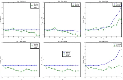
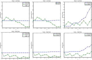
Here we report the error rates using three measures we defined for three other UCI data sets (Blake and Merz (1998)), Heart, Ionosphere and Sonar. Linear version of our formulation was used. Experiments were done with low noise (50% patterns with missing values) and high noise (90% patterns with missing values). The data sets were divided in the ratio 9:1, the larger set was used for training the nominal and robust classifiers while the smaller set was used as test data set. 50% of the feature values (chosen at random) were deleted from 50% of the training patterns (in the low noise case) and 90% of the training patterns (in the high noise case). Linear regression based model was used to fill in the missing values. Nominal classifier and robust classifiers with different values ofγwere trained using each such data set. Error rates were obtained for the test data set after deleting 50% of the feature values from each test pattern. The error rates reported here are over ten such randomized iterations.
The error rates as a function ofγare plotted in Figures 5,6 and 7. In case of actual error, the plots also show a horizontal line labeled ’clean’ which is the error rate on the actual data set without any missing values. In this case, we did not delete any feature values from the data set. Nominal classifiers were trained and testing was also done on complete test samples. Our aim was to see how close our robust classifier could get near the error rates obtained using the complete data set.
It can be seen that the robust classifier, with suitable amount of robustness comes very close to the error rates on the clean data set. Amongst the three error measures the worst case error, the last column of Figure 7, brings out the advantage of the robust classifier over the nominal classifier. Clearly with increasingγthe robust formulation gives dividends over the nominal classifier.
We also did experiments to compare the kernelized version of the formulation over the linear formulation. For this purpose, we generated a dataset as follows. The positive class was obtained by generating uniformly distributed points in a hypershpere inR5of unit radius centered at the origin. The negative class was obtained by generating uniformly distributed points in a annular band of thickness one, with the inner radius two, centered around the origin. In summary
y=
1 kxk ≤1 −1 2≤ kxk ≤3,
where x∈R5. An illustration of how such a dataset looks in two dimensions is given in the left of Figure 8. Hundred patterns were generated for each class. The data set was divided in the ratio 9:1. The larger part was used for training, the smaller part for testing. Three randomly chosen values were deleted from the training data set. The missing values were filled in using linear regression based strategy. We trained a classifier for different values ofγ. Actual Error was found out for both the kernelized version and the linear version of the formulation. The results reported here are over ten such randomized runs. Gaussian kernel(K(x,y) =exp(−qkx−yk2))was used in the case of kernelized formulation. The parameter q was chosen by cross validation. Spherical uncertainty was assumed in ˜K-space for samples with missing values in case of kernelized robust formulations.
Figure 8 shows actual error rates with linear nominal, linear robust, kernelized nominal and kernelized robust. It can be seen that the linear classifier has broken down, while the kernelized classifier has managed a smaller error rate. It can also be observed that the robust kernelized classi-fier has the least error rate.
8.2 Regression
0 0.2 0.4 0.6 0.8 1 1.2 1.4 0.2
0.28 0.36
Heart − Low Noise
γ
Actual Error
Nominal Robust Clean
0 0.2 0.4 0.6 0.8 1 1.2 1.4
0.2 0.28 0.36
γ
Expected Error
Heart − Low Noise
Nominal Robust
0 0.2 0.4 0.6 0.8 1 1.2 1.4
0.2 0.22 0.24 0.26 0.28 0.3 0.32 0.34 0.36
Heart − Low Noise
γ
Worst Case
Nominal Robust
0 0.2 0.4 0.6 0.8 1 1.2 1.4
0.2 0.28 0.36
Heart − High Noise
γ
Actual Error
Nominal Robust Clean
0 0.2 0.4 0.6 0.8 1 1.2 1.4
0.2 0.28 0.36
γ
Expected Error
Heart − High Noise
Nominal Robust
0 0.2 0.4 0.6 0.8 1 1.2 1.4
0.2 0.28 0.36
γ
Worst Case
Heart − High Noise
Nominal Robust
Figure 5: Error rates as a function ofγfor Heart. Patterns in the top row contained 50% missing variables, even ones 90%. From left to right — actual error, expected error, and worst case error.
imputed data. The obtained regression function will be called the nominal SVR. In this section we compare our formulations with nominal SVR on a toy dataset and one real world dataset in the linear setting. We also compared the kernelized formulations with the linear formulations.
The first set of results is on a toy data set consisting of 150 observations. Each observation consisted(y,x)pair where
y=w⊤x+b, w⊤= [1,2,3,4,5], b=−7.
Patterns x were generated from a Gaussian distribution with mean, µ=0, and randomly chosen covariance matrix,Σ. The results are reported for the following choice ofΣ:
0.1872 0.1744 0.0349 −0.3313 −0.2790 0.1744 0.4488 0.0698 −0.6627 −0.5580 0.0349 0.0698 0.1140 −0.1325 −0.1116 −0.3313 −0.6627 −0.1325 1.3591 1.0603 −0.2790 −0.5580 −0.1116 1.0603 0.9929
.