Learning to Classify Ordinal Data: The Data Replication Method

Learning to Classify Ordinal Data: The Data Replication Method

Jaime S. Cardoso [email protected]

INESC Porto, Faculdade de Engenharia, Universidade do Porto Campus da FEUP, Rua Dr. Roberto Frias, n 378

4200-465 Porto, Portugal

Joaquim F. Pinto da Costa [email protected]

Faculdade Ciˆencias Universidade Porto Rua do Campo Alegre, 687

4169-007 Porto, Portugal

Editor: Ralf Herbrich

Abstract

Classification of ordinal data is one of the most important tasks of relation learning. This paper introduces a new machine learning paradigm specifically intended for classification problems where the classes have a natural order. The technique reduces the problem of classifying ordered classes to the standard two-class problem. The introduced method is then mapped into support vector machines and neural networks. Generalization bounds of the proposed ordinal classifier are also provided. An experimental study with artificial and real data sets, including an application to gene expression analysis, verifies the usefulness of the proposed approach.

Keywords: classification, ordinal data, support vector machines, neural networks

1. Introduction

Predictive learning has traditionally been a standard inductive learning, where different sub-problem formulations have been identified. One of the most representative is classification, consisting on the estimation of a mapping from the feature space into a finite class space. Depending on the cardinality of the finite class space we are left with binary or multiclass classification problems. Finally, the presence or absence of a “natural” order among classes will separate nominal from ordinal problems.

Although two-class and nominal data classification problems have been thoroughly analysed in the literature, the ordinal sibling has not received nearly as much attention yet. Nonetheless, many real life problems require the classification of items into naturally ordered classes. The scenarios in-volved range from information retrieval (Herbrich et al., 1999a) and collaborative filtering (Shashua and Levin, 2002) to econometric modeling (Mathieson, 1995) and medical sciences (Cardoso et al., 2005). It is worth pointing out that distinct tasks of relational learning, where an example is no longer associated with a class or rank, which include preference learning and reranking (Shen and Joshi, 2005), are topics of research on their own.

piece of additional information—the order—may explain the widespread use of conventional meth-ods to tackle the ordinal data problem.

This work addresses this void by introducing in Section 2 the data replication method, a nonpara-metric procedure for the classification of ordinal data. The underlying paradigm is the extension of the original data set with additional variables, reducing the classification task to the well known two-class problem. Starting with the simpler linear case, already established in Cardoso et al. (2005), the section develops the nonlinear case; from there the method is extended to incorporate the procedure of Frank and Hall (2001). Finally, the generic version of the data replication method is presented, allowing partial constraints on variables.

In section 3 the data replication method is instantiated in two important machine learning algo-rithms: support vector machines and neural networks. A comparison is made with a previous SVM approach introduced by Shashua and Levin (2002), the minimum margin principle, showing that the data replication method leads essentially to the same solution, but with some key advantages. The section is concluded with a reinterpretation of the neural network model as a generalization of the ordinal logistic regression model.

Section 4 describes the experimental methodology and the algorithms under comparison; results are reported and discussed in the succeeding sections. Finally, conclusions are drawn and future work is outlined in Section 8.

2. The Data Replication Method

Assume that examples in a classification problem come from one of K ordered classes, labeled from

C1

to

C

K, corresponding to their natural order. Consider the training set{xi(k)}, where k=1, . . . ,K

denotes the class number, i=1, . . . , `k is the index within each class, and x(ik)∈Rp, with p the

dimension of the feature space. Let`=∑K<sub>k=1</sub>`kbe the total number of training examples.

Suppose that a K-class classifier was forced, by design, to have(K₋1)nonintersecting bound-aries, with boundary i discriminating classes

C1

, . . . ,

C

i against classes

C

i+1, . . . ,

C

K. As the

in-tersection point of two boundaries would indicate an example with three or more classes equally probable—not plausible with ordinal classes—this strategy imposes a sensible restriction. With this constraint emerges a monotonic model, where a better value in an attribute does not lead to a lower decision class. For the linear case, this translates into choosing the same weighted sum for all decisions—the classifier would be just a set of weights, one for each feature, and a set of thresholds, the scale in the weighted sum. By avoiding the intersection of any two boundaries, this model tries to capture the essence of the ordinal data problem. Additionally, we foresee a better generalization performance due to the reduced number of parameters to be estimated.

This rationale leads to a straightforward generalization of the two-class separating hyperplane (Shashua and Levin, 2002). Define(K₋1)hyperplanes that separate the training data into K ordered classes by modeling the ranks as intervals on the real line. The geometric interpretation of this approach is to look for (K₋1) parallel hyperplanes, represented by vector w_∈Rp and scalars

b1, . . . ,bK−1, such that the feature space is divided into K regions by the decision boundaries wtx+

br=0,r=1, . . . ,K−1.

2.1 Data Replication Method—the Linear Case1

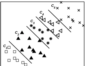
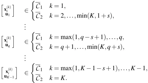
Before moving to the formal presentation of the data replication method, it is instructive to motivate the method by considering a hypothetical, simplified scenario, with five classes in R2. The plot of the data set is presented in Figure 1(a); superimposed is also depicted a reasonable set of four parallel hyperplanes separating the five classes.

C

1

C₂ C₃

C₄ C

5

(a) Plot of the data points. Also shown are reasonable class boundaries.

1-st

C1 {C2,C3}

2-nd

{C1,C2} {C3,C4}

3-rd

{C2,C3} {C4,C5}

4-th

{C3,C4} C5

(b) Classes involved in the hy-perplanes definition, for K=5,

s=2.

Figure 1: Toy model with 5 classes inR2.

The i-th hyperplane discriminates classes

C1

, . . . ,

C

i against classes

C

i+1, . . . ,

C

K. Due to the

order among classes, the i-th hyperplane is essentially determined by classes

C

i and

C

i+1. More generally, it can be said that the i-th hyperplane is determined by s classes to its ‘left’ and s classes to its ‘right’, with 1_≤s_≤K₋1. Naturally, for some of the hyperplanes, there will be less than

s classes to one (or both) of its sides. The i-th hyperplane has i classes on its left and (K₋i) on its right. Hence, for a chosen s value, we may say that classifier i depends on min(s,i) classes on its left—classes

C

k,k=max(i₋s+1,1), . . . ,i—and depends on min(s,K₋i)classes on its right— classes

C

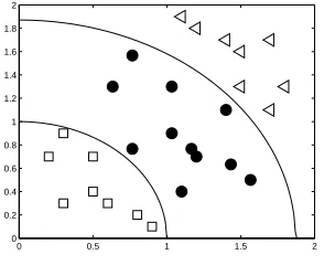
k,k=i+1, . . . ,min(i+1+s−1,i+1+K−i−1) =i+1, . . . ,min(i+s,K). The classes

involved in each hyperplane definition, for the five class data set with s=2, are illustrated in Figure 1(b).

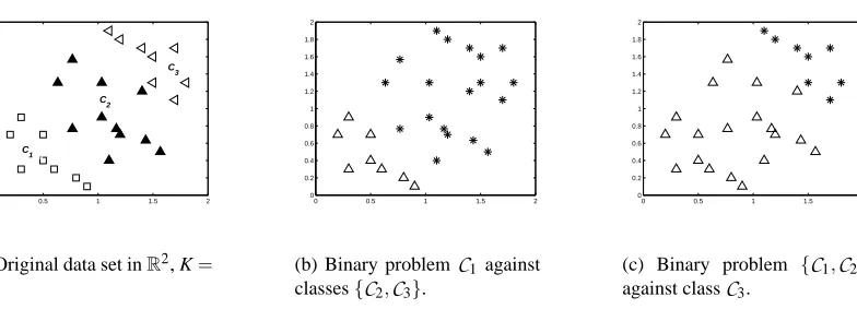
To start the presentation of the data replication method let us consider an even more simplified toy example with just three classes, as depicted in Figure 2(a). Here, the task is to find two parallel hyperplanes, the first one discriminating class

C1

against classes _{

C2

,

C3

_}(we are considering s=

K₋1=2 for the explanation) and the second discriminating classes _{

C1

,

C2

_} against class

C3.

These hyperplanes will correspond to the solution of two binary classification problems but with the additional constraint of parallelism—see Figure 2. The data replication method suggests solving both problems simultaneously in an augmented feature space.

0 0.5 1 1.5 2 0 0.2 0.4 0.6 0.8 1 1.2 1.4 1.6 1.8 2 C₁ C₂ C₃

(a) Original data set inR2, K=

3.

0 0.5 1 1.5 2 0 0.2 0.4 0.6 0.8 1 1.2 1.4 1.6 1.8 2

(b) Binary problemC1 against classes{C2,C3}.

0 0.5 1 1.5 2 0 0.2 0.4 0.6 0.8 1 1.2 1.4 1.6 1.8 2

(c) Binary problem {C1,C2} against classC3.

Figure 2: Binary problems to be solved simultaneously with the data replication method.

Using a transformation from the R2 initial feature-space to aR3 feature space, replicate each original point, according to the rule (see Figure 3(b)):

x_∈R2%

&

[x_h]_∈R3

[x 0]∈R3

, where h=const_∈R+.

Observe that any two points created from the same original point differ only in the new variable. Define now a binary training set in the new (higher dimensional) space according to (see Figure 3(c)):

h

x(_i1) 0

i ∈

C

1,

h

x(_i2) 0

i ,hx(_i3)

0

i

∈

C2

;

h

x(_i1)

h i

,hx(_i2)

h i

∈

C

1,

h

x(_i3)

h i

∈

C

2. (1)

In this step we are defining the two binary problems as a single binary problem in the augmented feature space. A linear two-class classifier can now be applied on the extended data set, yielding a hyperplane separating the two classes, see Figure 3(d). The intersection of this hyperplane with each of the subspace replicas can be used to derive the boundaries in the original data set, as illustrated in Figure 3(e).

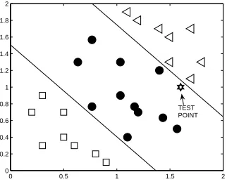
Although the foregoing analysis enables one to classify unseen examples in the original data set, classification can be done directly in the extended data set, using the binary classifier, without explicitly resorting to the original data set. For a given example _∈R2, classify each of its two replicas_∈R3, obtaining a sequence of two labels_{∈ {}

C

1,

C2

}2. From this sequence infer the class according to the rule

C1C

1=⇒

C1

,

C

2C1=⇒

C2

,

C

2C2=⇒

C3

.

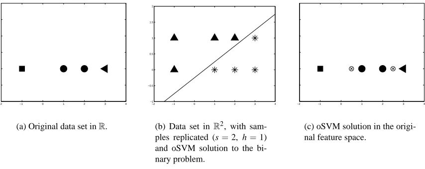
To exemplify, from the test point in Figure 3(a), create two replicas and classify them inR3 (high-lighted in Figure 3(d)). The first replica is classified as

C

2and the second as

C

1. Hence, the class predicted for the test point is

C2. This same class could have been obtained in the original feature

space, as represented in Figure 3(e).

0 0.5 1 1.5 2 0 0.2 0.4 0.6 0.8 1 1.2 1.4 1.6 1.8 2 TEST POINT

(a) Original data set inR2, K=3.

0 0.5 1 1.5 2 0 0.5 1 1.5 2 0 0.2 0.4 0.6 0.8 1 TEST POINT REPLICA 2 TEST POINT REPLICA 1

(b) Data set inR3, with samples replicated (h=

1). 0 0.5 1 1.5 2 0 0.5 1 1.5 2 0 0.2 0.4 0.6 0.8 1 TEST POINT REPLICA 1 TEST POINT REPLICA 2

(c) Transformation into a binary classification problem.

0 0.5

1 1.5

2 0 0.5

1 1.5 2 0 0.2 0.4 0.6 0.8 1 TEST POINT REPLICA 1 TEST POINT REPLICA 2

(d) Linear solution to the binary problem.

0 0.5 1 1.5 2 0 0.2 0.4 0.6 0.8 1 1.2 1.4 1.6 1.8 2 TEST POINT

(e) Linear solution in the original data set.

C

i+1, . . . ,

C

K (more generally, when parameterized by s, discriminating classes

C

k,k=max(i−s+

1,1), . . . ,i against classes

C

k,k=i+1, . . . ,min(i+s,K)). The additional variables, in number of

(K₋2), provide just the right amount of flexibility needed for having boundaries with the same direction but with different thresholds.

After the above exposition on a toy model, we will now formally describe a general K-class classifier for ordinal data classification. Define e0 as the sequence of(K₋2)zeros and eq as the

sequence of(K₋2) symbols 0, . . . ,0,h,0, . . . ,0, with h>0 in the q-th position. Considering the problem of separating K ordered classes

C1

, . . . ,

C

K with training set {x(ik)}, define a new binary

training data set inRp+K−2as

h

x(ik) e0

i ∈

(

C

1 k=1,

C

2 k=2, . . . ,min(K,1+s),

.. .

h

x(_ik) eq−1

i ∈

(

C

1 k=max(1,q−s+1), . . . ,q,

C

2 k=q+1, . . . ,min(K,q+s),

.. .

h

x(ik) eK₋2

i ∈

(

C

1 k=max(1,K−1−s+1), . . . ,K−1,

C

2 k=K,

(2)

where parameter s_{∈ {}1, . . . ,K₋1_}plays the role of bounding the number of classes defining each hyperplane. This setup allows controlling the increase of data points inherent to this method. The toy example in Figure 3(b) was illustrated with s=K₋1=2; by setting s=1 one would obtain the extended data set illustrated in Figure 4.

0 0.5

1 1.5

2 0 0.5

1 1.5

2 0

0.2 0.4 0.6 0.8 1

Figure 4: Toy data set replicated inR3, h=1, s=1.

original space gives rise to the(K−1)boundaries, in the form wtx+bi, with

bi= (

b if i=1,

h wp+i−1+b if i>1. Now, what possible sequences can one obtain?

Assume for now that the thresholds are correctly ordered as −b1≤ −b2≤. . .≤ −bK−1. Or,

equivalently, that 0_≥h wp+1≥h wp+2. . .≥h wp+K₋2. If the replica[eix]of a test point x is predicted as ¯

C1

, that is because ¯wt[eix] +b<0. But then also the replica [eix+1]is predicted as ¯

C1

because

0≥h wp+i≥h wp+i+1. One can conclude that the only K possible sequences and the corresponding predicted classes are

C

1,

C

1, . . . ,

C

1,

C1

=⇒

C1

,

C

2,

C

1, . . . ,

C

1,

C1

=⇒

C2

,

.. .

C

2,

C

2, . . . ,

C

2,

C1

=⇒

C

K−1,

C

2,

C

2, . . . ,

C

2,

C2

=⇒

C

K.

Henceforth, the target class can be obtained by adding one to the number of

C

2 labels in the se-quence. To emphasize, the process is depicted in Figure 5 for a data set in Rwith four classes.

The reduction technique presented here uses a binary classifier to make multiclass ordinal pre-dictions. Instead of resorting to multiple binary classifiers to make predictions in the ordinal prob-lem (as is common in reduction techniques from multiclass to binary probprob-lems), the data replication method uses a single binary classifier to classify(K−1)dependent replicas of a test point. A

perti-nent question is how the performance of the binary classifier translates into the performance on the ordinal problem. In Appendix A, a bound on the generalization error of the ordinal data classifier is expressed as a function of the error of the binary classifier.

The thresholds biwere assumed correctly ordered. It is not trivial to see how to keep them well

ordered with this standard data replication method, for s general. We present next an alternative method of replicating the data, in which constraints on the thresholds are explicitly incorporated in the form of extra points added to the training set. This formulation enforces ordered boundaries for

s values as low as 1, although compromising some of cleanliness in the interpretation as a binary

classification problem in the extended space.

2.2 Homogeneous Data Replication Method

With the data replication method just presented, the boundary in the extended space ¯wtx¯+b=0 has correspondence in the original space to the (K₋1) boundaries wtx+bi, with b1=b, bi =

h wp+i−1+b1,i=2, . . . ,K−1. It is notorious the asymmetry with respect to b1.

One could attain a symmetric formulation by introducing the well-known homogenous coordi-nates. That would lead to the addition of a new variable and to the restriction of linear boundaries going through the origin. The same result can be obtained by starting with a slightly different extension of the data set.

Define uqas the sequence of(K−1)symbols 0, . . . ,0,h,0, . . . ,0, with h>0 in the q-th position.

Considering the problem of separating K ordered classes

C1

, . . . ,

C

Kwith training set{x(ik)}, define

0 1 2 3 4 5 −1 −0.8 −0.6 −0.4 −0.2 0 0.2 0.4 0.6 0.8 1

(a) Original data set inR, K=4.

1 2 3 4 0 0.2 0.4 0.6 0.8 1 0 0.2 0.4 0.6 0.8 1 x3 x1 x2

(b) Data set inR3, with samples repli-cated (h=1).

1 2 3 4 0 0.2 0.4 0.6 0.8 1 0 0.2 0.4 0.6 0.8 1 x3 x1 x2

(c) Transformation into a binary clas-sification problem. 1 2 3 4 0 0.2 0.4 0.6 0.8 1 0 0.2 0.4 0.6 0.8 1 x1 x2 x3

(d) Linear solution to the binary prob-lem.

Figure 5: Proposed data extension model for a data set inR, with K=4.

h

x(_ik) u1

i ∈

(

C1

k=1,

C2

k=2, . . . ,min(K,1+s),

.. .

h

x(ik) uq

i ∈

(

C1

k=max(1,q−s+1), . . . ,q,

C2

k=q+1, . . . ,min(K,q+s),

.. .

h

x(_ik) uK−1

i ∈

(

C1

k=max(1,K₋1₋s+1), . . . ,K₋1,

C2

k=K.

Note that the homogeneous extended data set has dimension p+K₋1, as opposed to(p+K₋2) in the standard formulation of the data replication method. It also comes that bi =h wp+i, i=

1, . . . ,K₋1. Under the homogeneous approach, one has to look for a linear homogeneous boundary

The main reason for preferring the standard over the homogeneous formulation of the data replication method is that most of the existing linear binary classifiers are formulated in terms of non-homogeneous boundaries having the form ¯wtx¯+b=0, instead of ¯wtx¯=0. Therefore, some adaptation is required before applying existing linear binary classifiers to the homogeneous data replication method.

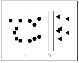
Homogeneous Data Replication Method with Explicit Constrains on the Thresholds

Unless one sets s=K₋1, the data replication method does not enforce ordered thresholds (we will return to this point later, when mapping to SVMs and neural networks). This is true for both the standard and the homogeneous formulations. Explicit constraints in the model’s formulation can be introduced to enforce the correct order. With the homogeneous formulation, those explicit constraints can take the form of additional(K₋2)points in the training set.

Consider the relation₋bi<−bi+1. This relation can be equivalently written as

−h wp+i<−h wp+i+1⇐⇒ −w¯t

_0p

ui

<₋w¯t

h

0p ui+1

i

⇐⇒w¯t

h

0p ui+1−ui

i <0.

As a result, constraining₋bi to be less than−bi+1is equivalent to correctly classify the point

h

0p ui+1−ui

i

in the

C1

class. It is interesting to note that this point is not in the subspace of any of the

data replicas. To introduce the(K₋2)explicit constraints on the thresholds, just enforce that the (K₋2)points

h

0p ui+1−ui

i

,i=1, . . . ,K₋2 are correctly classified in

C1

. Note that violations of these

constraints can not be allowed.

2.3 Data Replication Method—the Nonlinear Case

Previously, the data replication method was considered as a design methodology of a linear classi-fier for ordinal data. This section addresses scenarios where data is not linearly separable and for which the design of a linear classifier does not lead to satisfactory results. Therefore, the design of nonlinear classifiers emerges as a necessity. The only constraint to enforce during the design process is that boundaries should not intersect.

Inspired by the data replication method just presented, we now look for generic boundaries that are level curves of some nonlinear, real-valued function G(x) defined in the feature space. The (K−1)boundaries are defined as G(x) =bi,i=1, . . . ,K−1,bi∈R. It is worth emphasizing that

interpreting the decision boundaries as level curves of some (unknown) function does not result in loss of generality. For the linear version one take G(x) =wtx+b.

Once again, the search for nonintersecting, nonlinear boundaries can be carried out in the ex-tended space of the data replication method. First, extend and modify the feature space to a binary problem, as dictated by the data replication method. Next, search for a boundary G(x)defined in the extended space that results on(K₋1)boundaries G(x) =biwhen reverted to the original space.

The simplest form for G(x)is as a partially linear (nonlinear in the original variables but linear in the introduced variables) boundary G(x) =G(x) +wtei=0, with w∈RK−2, and x= [eix]. Notice that restricting the function G(x)to be linear in the(K₋2)added variables imposes automatically nonintersecting boundaries in the original space: boundaries will have the form G(x) +bi=0 with

bi = (

0 if i=1,

Although a partially linear function G(x)is the simplest to provide nonintersecting boundaries in the original space (level curves of some function G(x)), it is by no means the only type of function to provide them.

The intersection of the constructed high-dimensional boundary with each of the subspace repli-cas provides the desired(K₋1)boundaries. This approach is plotted in Figure 6 for the toy example. The #C2+1 rule can still be applied to predict the class of a test example directly in the extended feature space.

0 0.5

1 1.5

2 0

0.5 1

1.5 2 0

0.2 0.4 0.6 0.8 1

(a) Nonlinear solution to the binary prob-lem. G(x) =0.4(x₁2+x₂2−1) +x3

0 0.5 1 1.5 2 0

0.2 0.4 0.6 0.8 1 1.2 1.4 1.6 1.8 2

(b) Nonlinear solution in the original data set. G(x) =x2₁+x2₂−1

Figure 6: Nonlinear data extension model in the toy example.

The nonlinear extension of the homogeneous data replication method follows the same rationale as the standard formulation. Now the G(x) =G(x) +wtui=0 boundary, with w∈RK−1, must be

constrained such that G(0) =0_⇐⇒G(0) =0. Finally, the enforcement of ordered thresholds with the introduction of additional training points is still valid in the nonlinear case, as

G(h_ui+0p

1−ui i

) =G(0p) +wt(ui+1−ui) =h wp+i+1−h wp+i=bi+1−bi.

2.4 A General Framework

As presented so far, the data replication method allows only searching for parallel hyperplanes (level

curves in the nonlinear case) boundaries. That is, a single direction is specified for all boundaries.

In the quest for an extension allowing more loosely coupled boundaries, let us start by reviewing the method for ordinal data by Frank and Hall (2001).

2.4.1 THE METHOD OFFRANK AND HALL

Frank and Hall (2001) proposed to use (K₋1) standard binary classifiers to address the K-class ordinal data problem. Toward that end, the training of the i-th classifier is performed by converting the ordinal data set with classes

C1

, . . . ,

C

K into a binary data set, discriminating

C1

, . . . ,

C

i against

C

i+1, . . . ,

C

K. To predict the class value of an unseen instance, the(K−1) outputs are combined

Hall (2001) suggest to estimate the probability values of each of the K classes as

pC1 =1−p1,

p_Cj =pj−1−pj j=2,···,K−1,

pCK =pK−1.

Note however that this approach may lead to negative estimates of probability values. A solution to that problem is to identify the output pi of the i-th classifier with the conditional probability

p(

C

X>

C

i|

C

X>

C

i−1). This meaning can be exploited to rank the classes according to the following formulas:

p(

C

X >

C1

) =p1, pC1 =1−p1,

p(

C

X >

C

j) =pjp(

C

X>

C

j₋1), pCj = (1−pj)p(

C

X >

C

j−1) j=2,···,K−1,

p_CK =p(

C

X>

C

K−1).

Any binary classifier can be used as the building block of this scheme. Observe that, under our approach, the i-th boundary is also discriminating

C1

, . . . ,

C

i against

C

i+1, . . . ,

C

K; the major

difference lies in the independence of the boundaries found with Frank and Hall’s method. This independence is likely to lead to intersecting boundaries.

2.4.2 APARAMETERIZED FAMILY OF CLASSIFIERS

Thus far, nonintersecting boundaries have been motivated as the best way to capture ordinal relation among classes. That may be a too restrictive condition for problems where some features are not in relation with the ordinal property. Suppose then that the order of the classes is not totally reflected in a subset of the features. Without further information, it is unadvised to draw from them any ordinal information. It may be more advantageous to restrict the enforcing of the nonintersecting boundaries to the leftover features.

We suggest a generalization of the data replication method where the enforcement of noninter-secting boundaries is restricted only to the first j features, while the last p₋j features enjoy the

independence as materialized in the Frank and Hall’s method. Towards that end we start by showing how the independent boundaries approach of Frank and Hall can be subsumed in the data replication framework.

Instead of replicating the original train data set as expressed by Eq. (2), we indent to arrive at a strategy that still allows a single binary classifier to solve the(K₋1)classification problems simul-taneously, but yielding independent boundaries. If the boundaries are expected to be independent, each of the(K−1)data replicas of the original data should be made as ‘independent’ as possible.

Up to this point, when replicating the original data set, the original p variables were the first p variables of the p+K₋2 variables of the augmented data set, for each subspace replica, as seen in Eq. (2). Each of the(K−2)extra variables accounts for a different threshold term, while the fact that the original variables are ‘shared’ among the different replicas results in a common direction for all of the boundaries. The argument is that if the set of the original p features is mapped into a different set of p variables for each data replica, while keeping the (K₋2) extra variables to account for different thresholds, the binary classifier will return (almost) independent boundaries. It is worth noticing that this procedure increases the number of variables in the extended space to (K₋1)_×p+ (K₋2).

x(_i1) 02

0

∈

C1

,

x(_i2) 02

0

,

x(_i3) 02

0

∈

C

2,

₀₂

x(i1)

h

, ₀₂

x(i2)

h

∈

C

1,

₀₂

x(i3)

h

∈

C

2

where 02 is the sequence of 2 zeros. Intuitively, by misaligning variables involved in the deter-mination of different boundaries (variables in different subspaces), we are decoupling those same boundaries.

Proceeding this way, boundaries can be designed almost independently (the mapping on SVMs will clarify this issue). In the linear case we have now four parameters to estimate, the same as for two independent lines inR2_{. Intuitively, this new rule to replicate the data allows the estimation of} the direction of each boundary in essentially an independent way.

The general formulation in Eq. (2) becomes

x(_ik) 0p(K−2)

e0

∈ (

C

1 k=1,

C

2 k=2, . . . ,min(K,1+s),

.. .





0p(q−1)

x(ik) 0p(K−q−1)

eq−1 

 ∈

(

C

1 k=max(1,q−s+1), . . . ,q,

C

2 k=q+1, . . . ,min(K,q+s),

.. .

_0p(K

−2)

x(_ik) eK−2

∈

(

C

1 k=max(1,K−1−s+1), . . . ,K−1,

C

2 k=K,

(3)

where 0_∗is the sequence of∗zeros.

While the basic linear data replication method requires the estimation of (p₋1) + (K₋1) parameters, the new rule necessitates of (p−1)(K−1) + (K−1) = p(K−1), the same as the Frank and Hall approach; this corresponds to the number of free parameters in(K₋1)independent

p-dimensional hyperplanes. While this does not aim at being a practical alternative to Frank’s

method, it does pave the way for intermediate solutions, filling the gap between the totally coupled and totally independent boundaries.





x(_ik)(1: j) x(_ik)(j+1:p) 0(p−j)(K−2)

e0 

 ∈

(

C

1 k=1,

C

2 k=2, . . . ,min(K,1+s),

.. .



  

x(_ik)(1: j) 0(p−j)(q−1)

x(ik)(j+1:p) 0(p−j)(K−q−1)

eq−1 

 

 ∈

(

C

1 k=max(1,q−s+1), . . . ,q,

C

2 k=q+1, . . . ,min(K,q+s),

.. .





x(_ik)(1: j) 0(p−j)(K−2)

x(_ik)(j+1:p) eK−2



 ∈

(

C

1 k=max(1,K−1−s+1), . . . ,K−1,

C

2 k=K.

With this rule[p₋1₋(j₋1)](K₋1) + (K₋1) +j₋1, j_{∈ {}1, . . . ,p_}, parameters are to be estimated.

This general formulation of the data replication method allows the enforcement of only the amount of knowledge (constraints) that is effectively known a priori, building the right amount of parsimony into the model (see the pasture production experiment).

Now, in this general setting, we can no longer assume nonintersecting boundaries. Therefore, the space of features may be partitioned in more than K regions. To predict the class of an unseen instance we may estimate the probabilities of the K classes using the(K₋1)replicas, similarly to Frank and Hall (2001), or simply keep the #

C

2+1 rule.

3. Mapping the Data Replication Method to Learning Algorithms

In this section the data replication method just introduced is instantiated in two important machine learning algorithms: support vector machines and neural networks.

3.1 Mapping the Data Replication Method to SVMs

The learning task in a classification problem is to select a prediction function f(x)from a family of possible functions that minimizes the expected loss.

In the absence of reliable information on relative costs, a natural approach for unordered classes is to treat every misclassification as equally likely. This translates into adopting the non-metric indicator function l0₋1(f(x),y) =0 if f(x) =y and l0−1(f(x),y) =1 if f(x)6=y, where f(x)and

y are the predicted and true classes, respectively. Measuring the performance of a classifier using

the l0−1loss function is equivalent to simply considering the misclassification error rate. However, for ordered classes, losses that increase with the absolute difference between the class numbers are more natural choices in the absence of better information (Mathieson, 1995). This loss should be naturally incorporated during the training period of the learning algorithm.

A risk functional that takes into account the ordering of the classes can be defined as

R(f) =E

h ls

f(x(k)),k i

(4)

with

ls

f(x(k)),k

=min

|f(x(k))₋k_|,s

The empirical risk is the average of the number of mistakes, where the magnitude of a mistake is related to the total ordering: Rs_emp(f) =1

`∑Kk=1∑ `k

i=1ls

f(x(_ik)),k.

Arguing as Herbrich et al. (1999a), we see that the role of parameter s (bounding the loss in-curred in each example) is to allow for an incorporation of a priori knowledge about the probability of the classes, conditioned by x, P(

C

k|x). This can be treated as an assumption on the

concentra-tion of the probability around a “true” rank. Let us see how all this finds its place with the data replication method.

3.1.1 THEMINIMUMMARGINPRINCIPLE

Let us formulate the problem of separating K ordered classes

C1

, . . . ,

C

K in the spirit of SVMs.

Starting from the generalization of the two-class separating hyperplane presented in the beginning of previous section, let us look for(K₋1)parallel hyperplanes represented by vector w_∈Rpand scalars b1, . . . ,bK−1, such that the feature space is divided into K regions by the decision boundaries

wtx+br=0,r=1, . . . ,K−1.

Going for a strategy to maximize the margin of the closest pair of classes, the goal becomes to maximize min_|wtx+bi|/||w||. Recalling that an algebraic measure of the distance of a point to

the hyperplane wtx+b is given by(wtx+b)/_kw_k, we can scale w and bi so that the value of the

minimum margin is 2/_kw_k.

The constraints to consider result from the(K₋1)binary classifications related to each hyper-plane; the number of classes involved in each binary classification can be made dependent on a parameter s, as detailed in Section 2.1. For the hyperplane q_{∈ {}1, . . . ,K₋1_}, the constraints result as

−(wtx(_ik)+bq) ≥+1 k=max(1,q−s+1), . . . ,q,

+(wtx(_ik)+bq) ≥+1 k=q+1, . . . ,min(K,q+s).

(5)

Reasoning as in the two-class SVM for the non-linearly separable data set, the inequalities can be relaxed using slack variables and the cost function modified to penalise any failure to meet the original (strict) inequalities. The model becomes (where sgn(x)returns+1 if x is greater than zero; 0 if x equals zero;₋1 if x is less than zero)

min w,bi,ξi

1 2w

t_w+CK

∑

−1 q=1

min(K,q+s)

∑

k=max(1,q₋s+1)

`k

∑

i=1

sgn(ξ(_i,k_q))

s.t.

−(wtx(_ik)+b1) ≥+1−ξ(_i,k₁) k=1,

+(wtx(_ik)+b1) ≥+1−ξ(i,k1) k=2, . . . ,min(K,1+s),

.. .

−(wtx(_ik)+bq) ≥+1−ξ( k)

i,q k=max(1,q−s+1), . . . ,q,

+(wtx(_ik)+bq) ≥+1−ξ(_i,k_q) k=q+1, . . . ,min(K,q+s),

.. .

−(wtx(_ik)+bK−1) ≥+1−ξ(i,kK)₋1 k=max(1,K−s), . . . ,K−1, +(wtx(_ik)+bK−1) ≥+1−ξ(i,kK)−1 k=K,

ξ(k)

i,q ≥0.

Since each point x(_ik) is replicated 2 s times, it is also involved in the definition of 2 s boundaries; consequently, it can be shown to be misclassified min(_|f(x(_ik))₋k_|,s) =ls(f(x(_ik)),k)times, where

f(x(_ik)) is the class estimated by the model. As with the two-class example,

∑K−1

q=1∑

min(K,q+s)

k=max(1,q−s+1)∑

`k

i=1 sgn(ξ (k)

i,q) is an upper bound of ∑k∑ils(f(x

(k)

i ),k), proportional to the

empirical risk.2

However, optimization of the above is difficult since it involves a discontinuous function sgn(). As it is common in such cases, we choose to optimize a closely related cost function, and the goal becomes

min w,bi,ξi

1 2w

t_w+CK

∑

−1 q=1

min(K,q+s)

∑

k=max(1,q−s+1)

`k

∑

i=1

ξ(k)

i,q

subject to the same constraints as Eq. (6).

In order to account for different misclassification costs or sampling bias, the model can be extended to penalise the slack variables according to different weights in the objective function (Lin et al., 2002):

min w,bi,ξi

1 2w

t_w+K

∑

−1 q=1

min(K,q+s)

∑

k=max(1,q₋s+1)

`k

∑

i=1

C(_i,k_q)ξ(_i,k_q).

As easily seen, the proposed formulation resembles the fixed margin strategy in Shashua and Levin (2002). However, instead of using only the two closest classes in the constraints of an hyper-plane, more appropriate for the loss function l0−1(), we adopt a formulation that captures better the performance of a classifier for ordinal data.

Some problems were identified in the Shashua’s approach. Firstly, it is an incompletely specified model. In fact, although the direction of the hyperplanes w is unique under the above formulation (proceeding as Vapnik (1998) for the binary case), the scalars b1, . . . ,bK−1are not uniquely defined, as illustrated in Figure 7.

b

1 b2

Figure 7: Scalar b2is undetermined over an interval under the fixed margin strategy.

. . ._{≤ −}bK−1are not guaranteed in this case. Only under the setting s=K−1 the ordinal inequalities on the thresholds are automatically satisfied (Chu and Keerthi, 2005).

Lastly, although the formulation was constructed from the two-class SVM, it is no longer solv-able with the same algorithms. It would be interesting to accommodate this formulation under the two-class problem. That would allow the use of mature and optimized algorithms, developed for the training of support vector machines (Platt, 1998; Dong et al., 2005).

3.1.2 THE OSVM ALGORITHM

In order to get a better intuition of the general result, consider first the toy example previously presented. The binary SVM formulation for the extended and binarized training set can be described as with w= [w3w],w∈R2

minw,b 1₂wtw

s.t.

−(wt

h

x(_i1) 0

i

+b)_≥+1,

+(wt

h

x(_i2) 0

i

+b)_≥+1,

+(wthx(i3) 0

i

+b)_≥+1,

−(wt

h

x(_i1)

h i

+b)_≥+1,

−(wt

h

x(i2)

h i

+b)_≥+1,

+(wthx(i3)

h i

+b)_≥+1.

But because

(

wt[xi₀] =wtxi

wt[xi_h] =wtxi+w3h

and renaming b to b1and b+w3h to b2the formulation above simplifies to minw,b1,b2 1₂wtw+1₂(b2−b1)

2

h2

s.t.

−(wtx_i(1)+b1)≥+1, +(wtx(_i2)+b1)≥+1, +(wtx(_i3)+b1)≥+1,

−(wtx_i(1)+b2)≥+1,

−(wtx_i(2)+b2)≥+1, +(wtx(_i3)+b2)≥+1.

boundaries and maximizes the minimum of the margins—see Figure 8. The h parameter controls the trade-off between the objectives of maximizing the margin of separation and minimizing the distance between the hyperplanes. To reiterate, the data replication method enabled us to formulate

−2 −1 0 1 2 3 4

(a) Original data set inR.

−2 −1 0 1 2 3 4 −1

−0.5 0 0.5 1 1.5 2

(b) Data set inR2, with sam-ples replicated (s=2, h=1) and oSVM solution to the bi-nary problem.

−2 −1 0 1 2 3 4

(c) oSVM solution in the origi-nal feature space.

Figure 8: Effect of the regularization member in the oSVM solution.

the classification of ordinal data as a standard SVM problem and to remove the ambiguity in the solution by the introduction of a regularization term in the objective function.

The insight gained from studying the toy example paves the way for the formal presentation of the instantiation of the data replication method in SVMs. Consider a general extended data set, as defined in Eq. (2). After the simplifications and change of variables suggested for the toy example

(b=b1, b+hwp+i=bi+1, i=1, . . . ,K−2), the binary SVM formulation for this extended data set

yields

min w,bi,ξi

1 2w

t_w+ 1

h2

K−1

∑

i=2

(bi−b1)2 2 +C

K−1

∑

q=1

min(K,q+s)

∑

k=max(1,q₋s+1)

`k

∑

i=1

ξ(k)

i,q

with the same set of constraints as in Eq. (6).

This formulation for the high-dimensional data set matches the proposed formulation for ordinal data up to an additional regularization member in the objective function. This additional member is responsible for the unique determination of the thresholds.3

From the equivalence of the instantiation of the data replication method in SVMs and the model in Shashua and Levin (2002) and Chu and Keerthi (2005), the proof on the order of the thresholds is automatically valid for the oSVM algorithm with s=K₋1 (see the footnote on page 5 of Chu and Keerthi, 2005). The model parameter s cannot be chosen arbitrarily without additional constraints on the scalars b1, . . . ,bK₋1or some additional information about classes’ distribution.

To instantiate the homogeneous data replication method in support vector machines, some pop-ular algorithm for binary SVMs, such as the SMO algorithm, must be adapted for outputting a

so-3. Different regulation members could be obtained by different extensions of the data set. For example, if eq had

been defined as the sequence h, . . . ,h,0, . . . ,0, with q h’s and(K−2−q)0’s, the regularization member would be 1

2∑

i=K−1

i=2

(bi−bi−1)2

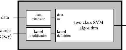
two-class SVM algorithm kernel

K(x,y)

data extensiondata

data in

kernel modification

kernel definition

Figure 9: oSVM interpretation of an ordinal multiclass problem as a two-class problem.

lution without the bias term. Moreover, kernels have to be restricted to those satisfying K(0,0) =0, as for instance the linear kernel or the homogeneous polynomial kernel K(x,y) = (xty)d_{. To}

im-plement the enforcement on the thresholds with additional training points, one can use a different value for the C parameter in these points, sufficiently high to make certain a correct classification. Alternatively, these points must not be relaxed with a slack variable in the SVM formulation.

Nonlinear Boundaries As explained before, the search for nonlinear level curves can be pur-sued in the extended feature space by searching for a partially linear function G(x) =G(x) +wt_e

i.

Since nonlinear boundaries are handled in the SVM context making use of the well known kernel trick, a specified kernel K(xi,xj)in the original feature space can be easily modified to K(xi,xj) =

K(xi,xj) +etxiexj in the extended space.

Summarizing, the nonlinear ordinal problem can be solved by extending the feature set and modifying the kernel function, as represented diagrammatically in Figure 9. Clearly, the extension to nonlinear decision boundaries follows the same reasoning as with the standard SVM (Vapnik, 1998).

It is true that the computational complexity of training a SVM model depends on the dimension of the input space, since the kernel functions contain the inner product of two input vectors for the linear or polynomial kernels or the distance of the two vectors for the Gaussian RBF kernel. However the matrix Q of inner products, with(Q)i j=K(xi,xj)can be computed once and kept in

memory. Even on problems with many training examples, caching strategies can be developed to provide a trade-off between memory consumption and training time (Joachims, 1998). Therefore, most of the increase in the computational complexity of the problem is due to the duplication of the data; more generally, for a K-class problem, the data set is increased at most (K−1) times,

O

(`(K₋1)).

min

w,bi,ξi

K−1

∑

k=1

1 2w

t_{(k p−p+1 : k p)w(k p−p+1 : k p) +} 1

h2

K−1

∑

i=2

(bi−b1)2

2 +C

K−1

∑

q=1

min(K,q+s)

∑

k=max(1,q−s+1)

`k

∑

i=1

ξ(k) i,q

s.t.

−(wt(1 : p)x(_ik)+b1) ≥+1−ξ(i,k1) k=1,

+(wt(1 : p)x_i(k)+b1) ≥+1−ξ(i,k1) k=2, . . . ,min(K,1+s),

.. .

−(wt(qp−p+1 : qp)x_i(k)+bq) ≥+1−ξ( k)

i,q k=max(1,q−s+1), . . . ,q,

+(wt(qp−p+1 : qp)x_i(k)+bq) ≥+1−ξ( k)

i,q k=q+1, . . . ,min(K,q+s),

.. . −(wt_{((K−1)p−p+1 :(K−1)p)x}(k)

i +bK₋1) ≥+1−ξ(_i,k_K)₋₁ k=max(1,K−s), . . . ,K−1,

+(wt_{((K−1)p−p+1 :(K−1)p)x}(k)

i +bK₋1) ≥+1−ξ_i(_,k_K)₋₁ k=K,

ξ(k) i,q ≥0.

If the regularization term _h12∑ K−1

i=2

(bi−b1)2

2 is zero (in practice, small enough), the optimization problem could then be broken in(K₋1)independent optimization problems, reverting to the

pro-cedure of Frank and Hall (2001).

3.2 Mapping the Data Replication Method to NNs

When the nonlinear data replication method was formulated, the real-valued function G(x) was defined arbitrarily. Nonintersecting boundaries were enforced by making use of a partially linear function G(x) =G(x) +wtei defined in the extended space. Setting G(x)as the output of a neural

network, a flexible architecture for ordinal data can be devised, as represented diagrammatically in Figure 10. Because G(x)an arbitrary real-valued function, it can be set as the output of a generic neural network with a single output. In Figure 10 G(x) is represented as the output of a generic feedforward network. This value is then linearly combined with the added(K₋2)components to produce the desired G(x)function.

For the simple case of searching for linear boundaries, the overall network simplifies to a single neuron with p+K₋2 inputs. A less simplified model, also used in the conducted experiments, is to consider a single hidden layer, as depicted in Figure 11. Note that this architecture can be obtained from Figure 10 by collapsing layers 2 to N₋1 into layer N, a valid operation when activation functions f2to fN−1are all linear.

Similarly to the SVM mapping, it is possible to show that, if we allow the samples in all the classes to contribute errors for each threshold, by setting s=K₋1, the order inequalities on the thresholds are satisfied automatically, in spite of the fact that such constraints on the thresholds are not explicitly included in the formulation. Refer to Appendix B for the detailed proof.

The mapping of the homogeneous data replication method to neural networks is easily realized. In order to obtain G(0) =0, just remove the biases inputs, represented in Figure 10, and restrict the activation functions fi()to those verifying fi(0) =0. The constrains on the thresholds in form

Generic neural network

+ activationfunction

fN

+ activationfunction

fN−1

+ activationfunction

fN−2

+ activationfunction

fN−2

+ activationfunction

f1

+ activationfunction

f1

x1

xp

xp+1

xp+K−2

G(x)

binary

classifier bias

bias

bias bias

bias

bias

Figure 10: Data replication method for neural networks (oNN).

+ activationfunction

fN

+ activationfunction

f1

+ activationfunction

f1

x1

xp

xp+1

xp+K−2

binary classifier

bias bias

bias

Figure 11: Simplified oNN model for neural networks.

3.2.1 ORDINALLOGISTICREGRESSIONMODEL

Here we provide a probabilistic interpretation for the ordinal neural network model just introduced. The traditional statistical approach for ordinal classification models the cumulative class probability

Pk=p(C≤k|x)by

logit(Pk) =Φk−G(x)⇔Pk=logsig(Φk−G(x)), k=1, . . . ,K−1 (7)

Remember that logit(y) =ln₁₋y_y, logsig(y)=₁₊1_e−y and logsig(logit(y)) =y.

For the linear version (McCullagh, 1980; McCullagh and Nelder, 1989) we take G(x) =wtx. Mathieson (1995) presents a nonlinear version by letting G(x) be the output of a neural network. However other setups can be devised. Start by observing that in Eq. (7) we can always assume

−6 −4 −2 0 2 4 6 −6

−4 −2 0 2 4 6

Figure 12: Decision boundaries for the oNN with 3 units in the hidden layer, for a synthetic data set from Mathieson (1995).

C1

=_◦,

C2

=,

C3

=/,

C4

=_∗

G(x)and(K−2)cut points. By fixing fN() =logsig()as the activation function in the output layer

of our oNN network, we can train the network to predict the values Pk(x), when fed with x= [ekx−1],

k=1, . . . ,K₋1 . By setting

C

1=1 and

C

2=0 we see that the extended data set as defined in Eq.

(2) can be used to train the oNN network. The predicted cut points are simply the weights of the connection of the added K₋2 components, scaled by h.

Illustrating this model with the synthetic data set from Mathieson (1995), we attained the deci-sion boundaries depicted in Figure 12.

3.3 Summation

The data replication method has some advantages over standard algorithms presented in the litera-ture for the classification of ordinal data:

• It has an interesting and intuitive geometric interpretation. It provides a new conceptual framework integrating disparate algorithms for ordinal data classification: Chu and Keerthi (2005) algorithm, Frank and Hall (2001), ordinal logistic regression.

• While the algorithm presented in Shashua and Levin (2002); Chu and Keerthi (2005) is only formulated for SVMs, the data replication method is quite generic, with the possibility of being instantiated in different classes of learning algorithms, ranging from SVMs (or other kernel based approaches) to neural networks or something as simple as the Fisher method.

4. Experimental Methodology

In the following sections, experimental results are provided for several models based on SVMs and NNs, when applied to diverse data sets, ranging from synthetic to real ordinal data, and to a problem of feature selection. Here, the set of models under comparison is presented and different assessment criteria for ordinal data classifiers are examined.

4.1 Neural Network Based Algorithms

We compare the following algorithms:

• Conventional neural network (cNN). To test the hypothesis that methods specifically targeted for ordinal data improve the performance of a standard classifier, we tested a conventional feed forward network, fully connected, with a single hidden layer, trained with the special activation function softmax.

• Pairwise NN (pNN): Frank and Hall (2001) introduced a simple algorithm that enables stan-dard classification algorithms to exploit the ordering information in ordinal prediction prob-lems. First, the data is transformed from a K-class ordinal problem to(K₋1)binary prob-lems. To predict the class value of an unseen instance the probabilities of the K original classes are estimated using the outputs from the(K₋1)binary classifiers.

• Costa (1996), following a probabilistic approach, proposes a neural network architecture (iNN) that exploits the ordinal nature of the data, by defining the classification task on a suitable space through a “partitive approach”. It is proposed a feedforward neural network with(K₋1)outputs to solve a K-class ordinal problem. The probabilistic meaning assigned to the network outputs is exploited to rank the elements of the data set.

• Regression model (rNN): as stated in the introduction, regression models can be applied to solve the classification of ordinal data. A common technique for ordered classes is to estimate by regression any ordered scores s1≤. . ._≤sK by replacing the target class

C

iby the score si.

The simplest case would be setting si=i,i=1, . . . ,K (Mathieson, 1995; Moody and Utans,

1995; Agarwal et al., 2001). A neural network with a single output was trained to estimate the scores. The class variable

Cx

was replaced by the score sx = Cx−_K0.5 before applying the regression algorithm. These scores correspond to take as target the midvalues of K equal-sized intervals in the range[0,1). The adopted scores are suitable for a sigmoid output transfer function, which always outputs a value in(0,1). In the test phase, if a test query obtains the answer ˆsxthe corresponding class is predicted as ˆ

Cx

=bK ˆsxc+1.

• Proposed ordinal method (oNN), based on the standard data extension technique, as previ-ously introduced.

Experiments with neural networks were carried out in Matlab 7.0 (R14), making use of the Neural Network Toolbox. All models were configured with a single hidden layer and trained with Levenberg-Marquardt back propagation method, over at most 2000 epochs.

4.2 SVM Based Algorithms

• A conventional multiclass SVM formulation (cSVM), as provided by the software imple-mentation LIBSVM 2.8., based on the one-against-one decomposition. The one-against-one decomposition transforms the multiclass problem into a series of K(K₋1)/2 binary subtasks that can be trained by a binary SVM. Classification is carried out by a voting scheme.

• Pairwise SVM (pSVM): mapping in support vector machines the strategy of Frank and Hall (2001) above mentioned for the pNN model.

• Regression SVM (rSVM): The considered class of support vector regression was that ofν -SVR Scholkopf et al. (2000), as provided by the software implementation LIBSVM 2.8. Note that the model was trained to estimate the scores sxas defined before in respect to the rNN model. Becauseν-SVR does not guarantee outputs∈[0,1), the predicted class ˆ

Cx

=_bK ˆsxc+1 was properly cropped.

• Proposed ordinal method (oSVM), based on the standard data extension technique, as previ-ously introduced.

All support vector machine models were implemented in C++, using as core the software im-plementation provided by LIBSVM 2.8.

4.3 Measuring the Performance of Ordinal Data Classifiers

Having built a classifier, the obvious question is “how good is it?”. This begs the question of what we mean by good. A common approach is to treat every misclassification as equally costly, adopt-ing the misclassification error rate (MER) criterion to measure the performance of the classifier. However, as already expressed, losses that increase with the absolute difference between the class numbers capture better the fundamental structure of the ordinal problem. The mean absolute devia-tion (MAD) criterion takes into account the degree of misclassificadevia-tion and is thus a richer criterion than MER. The loss function corresponding to this criterion is l(f(x),y) =_|f(x)₋y_|. A variant of the above MAD measure is the mean square error (MSE), where the absolute difference is replaced by the square of the difference, l(f(x),y) = (f(x)₋y)2_.

Still, all these measures depend on the number assigned to each class, which is somewhat ar-bitrary. In order to try to avoid the influence of the numbers chosen to represent the classes on the performance assessment, we can look only at the order relation between true and predicted class numbers. The use of Spearman (rs) and Kendall’s tau-b (τb) coefficients, nonparametric rank-order

correlation coefficients well established in the literature (Press et al., 1992) are a step forward in that direction.

To get rsstart by ranking the two vectors of true and predicted classes. Ranking is achieved

by giving the ranking ‘1’ to the biggest number in a vector, ‘2’ to the second biggest value and so on. Obviously, there will be many examples in the class vector with common values; when ranking, those examples are replaced by average ranks. If R and Q represent two rank vectors, then

rs= ∑

(Ri−R¯)(Qi−Q¯) p

∑(Ri−R¯)2∑(Qi−Q¯)2

.

To define τb, start with the N data points (

Cxi

,

Cxi

ˆ ),i=1, . . . ,N, associated with the true and

et al. (1992), we call a pair(i,j)concordant if the relative ordering of the true classes

Cxi

and

Cxj

is the same as the relative ordering of the predicted classes ˆ

Cxi

and ˆ

Cxj

. We call a pair discordant if the relative ordering of the true classes is opposite from the relative ordering of the predicted classes. If there is a tie in either the true or predicted classes, then we do not call the pair either concordant or discordant. If the tie is in the true classes, we will call the pair an “extra true pair”, et. If the tie is in

the predicted classes, we will call the pair an “extra predicted pair”, ep. If the tie is both on the true

and the predicted classes, we ignore the pair. Theτbcoefficient can be computed as

τb=

concordant−discordant √

concordant+discordant+et p

concordant+discordant+ep .

Although insensitive to the number assigned to each class, both rsandτbare in fact more appropriate

for pairwise ranking rather than to ordinal regression, due to their failure to detect bias errors. In fact, if the predicted class is always a shift by a constant value of the true class, both indices will report perfect performance of the classifier.

Without a clear advantage of one criterion over the others, we decided on employing all the abovementioned assessment criteria in the conducted experiments.

5. Results for Synthetic Data

In a first comparative study we generated a synthetic data set in a similar way to Herbrich et al. (1999b). We generated 1000 example points x= [x1 x2]t uniformly at random in the unit square [0,1]_×[0,1]_⊂R2. Each point was assigned a rank y from the set_{1,2,3,4,5_}, according to

y= min

r∈{1,2,3,4,5}{r : br−1<10(x1−0.5)(x2−0.5) +ε <br},

(b0,b1,b2,b3,b4,b5) = (−∞,−1,−0.1,0.25,1,+∞).

whereε_∼N(0; 0.1252)simulates the possible existence of error in the assignment of the true class to x. Figure 13(a) depicts the 14.2% of examples which were assigned to a wrong class after the addition ofε. The unbalanced distribution of the random variable is shown is Figure 13(b).

In order to compare the different algorithms, we randomly split 100 times the data set into training, validation and test sets. Each model parameterization, namely the C parameter for SVMs (we tried values of the form C=1.25i_{, where i∈ {−8, . . . ,40}) and the number of neurons in the}

hidden layer for networks (varied from 0 to 10), was selected in accordance with the best mean performance over the 100 setups of the validation set. This was repeated taking`<sub>∈ {</sub>20,40,80<sub>}</sub>for size of the training set,`for the validation set and 1000₋2_×`for the test set. The test results for SVMs are shown in Table 1, for the MAD criterion.

We also investigated the other introduced criteria to assess models’ relative performance. Re-sults depicted in Figure 14 for this synthetic data set are representative of the agreement observed throughout the experimental study. All indices portrayed essentially the same relative models’ per-formance. For this reason, we shall restrict in the following to present only the results for the MAD criterion, possibly the most meaningful criterion for the ordinal regression problem.