Exponentiated Gradient Algorithms for Conditional Random Fields and Max-Margin Markov Networks

Exponentiated Gradient Algorithms for Conditional Random Fields

and Max-Margin Markov Networks

Michael Collins∗ [email protected]

Amir Globerson∗ [email protected]

Terry Koo∗ [email protected]

Xavier Carreras [email protected]

Computer Science and Artificial Intelligence Laboratory Massachusetts Institute of Technology

Cambridge, MA 02139, USA

Peter L. Bartlett [email protected]

University of California, Berkeley

Division of Computer Science and Department of Statistics Berkeley, CA 94720, USA

Editor: John Lafferty

Abstract

Log-linear and maximum-margin models are two commonly-used methods in supervised machine learning, and are frequently used in structured prediction problems. Efficient learning of parameters in these models is therefore an important problem, and becomes a key factor when learning from very large data sets. This paper describes exponentiated gradient (EG) algorithms for training such models, where EG updates are applied to the convex dual of either the log-linear or max-margin objective function; the dual in both the log-linear and max-max-margin cases corresponds to minimizing a convex function with simplex constraints. We study both batch and online variants of the algorithm, and provide rates of convergence for both cases. In the max-margin case, O(1

ε)EG

updates are required to reach a given accuracyεin the dual; in contrast, for log-linear models only O(log(1_ε))updates are required. For both the max-margin and log-linear cases, our bounds suggest that the online EG algorithm requires a factor of n less computation to reach a desired accuracy than the batch EG algorithm, where n is the number of training examples. Our experiments confirm that the online algorithms are much faster than the batch algorithms in practice. We describe how the EG updates factor in a convenient way for structured prediction problems, allowing the algorithms to be efficiently applied to problems such as sequence learning or natural language parsing. We perform extensive evaluation of the algorithms, comparing them to L-BFGS and stochastic gradient descent for log-linear models, and to SVM-Struct for max-margin models. The algorithms are applied to a multi-class problem as well as to a more complex large-scale parsing task. In all these settings, the EG algorithms presented here outperform the other methods.

Keywords: exponentiated gradient, log-linear models, maximum-margin models, structured pre-diction, conditional random fields

1. Introduction

Structured prediction problems involve learning to map inputs x to labels y, where the labels have rich internal structure, and where the set of possible labels for a given input is typically exponential in size. Examples of structured prediction problems include sequence labeling and natural language parsing. Several models that implement learning in this scenario have been proposed over the last few years, including log-linear models such as conditional random fields (CRFs, Lafferty et al., 2001), and maximum-margin models such as maximum-margin Markov networks (Taskar et al., 2004a).

For both log-linear and max-margin models, learning is framed as minimization of a regularized loss function which is convex. In spite of the convexity of the objective function, finding the optimal parameters for these models can be computationally intensive, especially for very large data sets. This problem is exacerbated in structured prediction problems, where the large size of the set of possible labels adds an additional layer of complexity. The development of efficient optimization algorithms for learning in structured prediction problems is therefore an important problem.

In this paper we describe learning algorithms that exploit the structure of the dual optimization problems for log-linear and max-margin models. For both log-linear and max-margin models the dual problem corresponds to the minimization of a convex function Q subject to simplex constraints (Jaakkola and Haussler, 1999; Lebanon and Lafferty, 2002; Taskar et al., 2004a). More specifically, the goal is to find

argmin

∀i,ui∈∆

Q(u1,u2, . . . ,un), (1)

where n is the number of training examples, each uiis a vector of dual variables for the i’th training

example, and Q(u)is a convex function.1 The size of each vector ui is|

Y

|, where

Y

is the set of

possible labels for any training example. Furthermore, ui is constrained to belong to the simplex of

distributions over

Y

, defined as:

∆=

(

p∈R|Y|: py≥0 ,

∑

y∈Y

py=1 )

. (2)

Thus each ui is constrained to form a distribution over the set of possible labels. The max-margin

and log-linear problems differ only in their definition of Q.

The algorithms in this paper make use of exponentiated gradient (EG) updates (Kivinen and Warmuth, 1997) in solving the problem in Eq. 1, in particular for the cases of log-linear or max-margin models. We focus on two classes of algorithms, which we call batch and online. In the batch case, the entire set of uivariables is updated simultaneously at each iteration of the algorithm;

in the online case, a single ui variable is updated at each step. The “online” case essentially

cor-responds to coordinate-descent on the dual function Q, and is similar to the SMO algorithm (Platt, 1998) for training SVMs. The online algorithm has the advantage of updating the parameters after every sample point, rather than after making a full pass over the training examples; intuitively, this should lead to considerably faster rates of convergence when compared to the batch algorithm, and indeed our experimental and theoretical results support this intuition. A different class of online algorithms consists of stochastic gradient descent (SGD) and its variants (e.g., see LeCun et al., 1998; Vishwanathan et al., 2006). In contrast to SGD, however, the EG algorithm is guaranteed to

improve the dual objective at each step, and this objective may be calculated after each example without performing a pass over the entire data set. This is particularly convenient when making a choice of learning rate in the updates.

We describe theoretical results concerning the convergence of the EG algorithms, as well as experiments. Our key results are as follows:

• For the max-margin case, we show that O(1

ε)time is required for both the online and batch

algorithms to converge to withinε of the optimal value of Q(u). This is qualitatively sim-ilar to recent results in the literature for max-margin approaches (e.g., see Shalev-Shwartz et al., 2007). For log-linear models, we show convergence rates of O(log(1

ε)), a significant

improvement over the max-margin case.

• For both the max-margin and log-linear cases, our bounds suggest that the online algorithm requires a factor of n less computation to reach a desired accuracy, where n is the number of training examples. Our experiments confirm that the online algorithms are much faster than the batch algorithms in practice.

• We describe how the EG algorithms can be efficiently applied to an important class of struc-tured prediction problems where the set of labels

Y

is exponential in size. In this case the number of dual variables is also exponential in size, making algorithms which deal directly with the ui variables intractable. Following Bartlett et al. (2005), we focus on a formulation

where each label y is represented as a set of “parts”, for example corresponding to labeled cliques in a max-margin network, or context-free rules in a parse tree. Under an assumption that part-based marginals can be calculated efficiently—for example using junction tree algo-rithms for CRFs, or the inside-outside algorithm for context-free parsing—the EG algoalgo-rithms can be implemented efficiently for both max-margin and log-linear models.

• In our experiments we compare the online EG algorithm to various state-of-the-art algo-rithms. For log-linear models, we compare to the L-BFGS algorithm (Byrd et al., 1995) and to stochastic gradient descent. For max-margin models we compare to the SVM-Struct algorithm of Tsochantaridis et al. (2004). The methods are applied to a standard multi-class learning problem, as well as to a more complex natural language parsing problem. In both settings we show that the EG algorithm converges to the optimum much faster than the other algorithms.

• In addition to proving convergence results for the definition of Q(u)used in max-margin and log-linear models, we give theorems which may be useful when optimizing other definitions of Q(u)using EG updates. In particular, we give conditions for convergence which depend on bounds relating the Bregman divergence derived from Q(u)to the Kullback-Leibler diver-gence. Depending on the form of these bounds for a particular Q(u), either O(1

ε)or O(log(1ε))

rates of convergence can be derived.

online cases. Section 6 discusses related work. Sections 7 and 8 give experiments, and Section 9 discusses our results.

This work builds on previous work described by Bartlett et al. (2005) and Globerson et al. (2007). Bartlett et al. (2005) described the application of the EG algorithm to max-margin param-eter estimation, and showed how the method can be applied efficiently to part-based formulations. Globerson et al. (2007) extended the approach to log-linear parameter estimation, and gave new convergence proofs for both max-margin and log-linear estimation. The work in the current paper gives several new results. We prove rates of convergence for a randomized version of the EG online algorithm; previous work on EG algorithms had not given convergence rates for the online case. We also report new experiments, including experiments with the randomized strategy. Finally, the O(log(1

ε))convergence rates for the log-linear case are new. The results in Globerson et al. (2007)

gave O(1

ε)rates for the batch algorithm for log-linear models, and did not give any theoretical rates

of convergence for the online case.

2. Primal and Dual Problems for Regularized Loss Minimization

In this section we present the log-linear and max-margin optimization problems for supervised learning. For each problem, we describe the equivalent dual optimization problem, which will form the core of our optimization approach.

2.1 The Primal Problems

Consider a supervised learning setting with objects x∈

X

and labels y∈

Y

.2 In the structured learning setting, the labels may be sequences, trees, or other high-dimensional data with internal structure. Assume we are given a function f(x,y):

X

×

Y

→Rd that maps(x,y)pairs to feature vectors. Our goal is to construct a linear prediction rule

h(x,w) =argmax

y∈Y

w·f(x,y),

with parameters w∈Rd, such that h(x,w) is a good approximation of the true label of x. The parameters w are learned by minimizing a regularized loss

L

(w;{(xi,yi)}ni=1,C) =

n

∑

i=1

`(w,xi,yi) +

C 2kwk

2_,

defined over a labeled training set{(xi,yi)}n_i=1. Here C>0 is a constant determining the amount of

regularization. The function`measures the loss incurred in using w to predict the label of xi, given

that the true label is yi.

In this paper we will consider two definitions for `(w,xi,yi). The first definition, originally

introduced by Taskar et al. (2004a), is a variant of the hinge loss, and is defined as follows:

`MM(w,xi,yi) =max

y∈Y

h

e(xi,yi,y)−w·(f(xi,yi)−f(xi,y)) i

. (3)

Here e(xi,yi,y) is some non-negative measure of the error incurred in predicting y instead of yi

as the label of xi. We assume that e(xi,yi,yi) =0 for all i, so that no loss is incurred for correct

prediction, and therefore `MM(w,xi,yi) is always non-negative. This loss function corresponds to

a maximum-margin approach, which explicitly penalizes training examples for which, for some y6=yi,

w·(f(xi,yi)−f(xi,y))<e(xi,yi,y).

The second loss function that we will consider is based on log-linear models, and is commonly used in conditional random fields (CRFs, Lafferty et al., 2001). First define the conditional distri-bution

p(y|x; w) = 1

Zx

ew·f(x,y),

where Zx=∑yew·f(x,y)is the partition function. The loss function is then the negative log-likelihood

under the parameters w:

`LL(w,xi,yi) =−log p(yi|xi; w).

The function

L

is convex in w for both definitions `MM and`LL. Furthermore, in both cases

minimization of

L

can be re-cast as optimization of a dual convex problem. The dual problems in the two cases have a similar structure, as we describe in the next two sections.

2.2 The Log-Linear Dual

The problem of minimizing

L

with the loss function`LLcan be written as

P-LL : w∗=argmin

w

∑

_i

−log p(yi|xi; w) +

C 2kwk

2_.

This is a convex optimization problem, and has an equivalent convex dual which was derived by Lebanon and Lafferty (2002). Denote the dual variables by ui,ywhere i=1, . . . ,n and y∈

Y

. We

also use u to denote the set of all variables, and uithe set of all variables corresponding to a given i.

Thus u= [u1, . . . ,un]. We assume u is a column vector. Define the function QLL(u)as

QLL(u) =

∑

i

∑

y

ui,ylog ui,y+

1

2Ckw(u)k 2_,

where

w(u) =

∑

i

∑

y

ui,ygi,y,

and where gi,y=f(xi,yi)−f(xi,y). We shall find the following matrix notation convenient:

QLL(u) =

∑

i

∑

y

ui,ylog ui,y+

1 2u

T_{Au, (4)}

where A is a matrix of size n|

Y

| ×n|

Y

|indexed by pairs(i,y), and A_(i,y),(j,z)= 1

Cgi,y·gj,z.

In what follows we denote the set of distributions over

Y

, that is, the|

Y

|-dimensional probabil-ity simplex, by∆, as in Eq. 2. The Cartesian product of n distributions over

Y

will be denoted by

∆n_{. The dual optimization problem is then}

D-LL : u∗= argmin QLL(u)

The minimum of D-LL is equal to−1 times the minimum of P-LL. The duality between P-LL and D-LL implies that the primal and dual solutions satisfy Cw∗=w(u∗).

2.3 The Max-Margin Dual

When the loss is defined using`MM(w,xi,yi), the primal optimization problem is as follows:

P-MM : w∗=argmin

w

∑

_i

max

y h

e(xi,yi,y)−w·(f(xi,yi)−f(xi,y)) i

+C

2kwk 2_.

The dual of this minimization problem was derived in Taskar et al. (2004a) (see also Bartlett et al., 2005). We first define the dual objective

QMM(u) =−bTu+

1 2u

T_{Au. (5)}

Here, the matrix A is as defined above and b∈Rn|Y| is a vector defined as bi,y =e(xi,yi,y). The

convex dual for the max-margin case is then given by

D-MM : u∗= argmin QMM(u)

s.t. u∈∆n_.

The minimum of D-MM is equal to−1 times the minimum of P-MM. (Note that for D-MM the minimizer u∗may not be unique; in this case we take u∗to be any member of the set of minimizers of QMM(u)). The optimal primal parameters are again related to the optimal dual parameters, through

Cw∗=w(u∗). Here again the constraints are that uiis a distribution over

Y

for all i.

It can be seen that the D-LL and D-MM problems have a similar structure, in that they both involve minimization of a convex function Q(u) over the set ∆n. This will allow us to describe algorithms for both problems using a common framework.

3. Exponentiated Gradient Algorithms

In this section we describe batch and online algorithms for minimizing a convex function Q(u)

subject to the constraints u∈∆n_{. The algorithms can be applied to both the D-LL and D-MM}

optimization problems that were introduced in the previous section. The algorithms we describe are based on exponentiated gradient (EG) updates, originally introduced by Kivinen and Warmuth (1997) in the context of online learning algorithms.3

The EG updates rely on the following operation. Given a sequence of distributions u∈∆n_{, a}

new sequence of distributions u0 can be obtained as

u0_i,y= 1

Zi

ui,ye−η∇i,y,

where∇i,y=∂Q_∂ui(u_,y), Zi=∑yˆui,yˆe−η∇i,yˆis a partition function ensuring normalization of the distribu-tion u0_i, and the parameterη>0 is a learning rate. We will also use the notation u0_i,y ∝ui,ye−η∇i,y

where the partition function should be clear from the context.

Clearly u0∈∆n_{by construction. For the dual function Q}

LL(u)the gradient is

∇i,y=1+log ui,y+

1

Cw(u)·gi,y,

and for QMM(u)the gradient is

∇i,y=−bi,y+

1

Cw(u)·gi,y.

In this paper we will consider both parallel (batch), and sequential (online) applications of the EG updates, defined as follows:

• Batch: At every iteration the dual variables uiare simultaneously updated for all i=1, . . . ,n.

• Online: At each iteration a single example k is chosen uniformly at random from{1, . . . ,n} and ukis updated to give u0_k. The dual variables uifor i6=k are left unchanged.

Pseudo-code for the two schemes is given in Figures 1 and 2. From here on we will refer to the batch and online EG algorithms applied to the log-linear dual as LLEG-Batch, and LLEG-Online respectively. Similarly, when applied to the max-margin dual, they will be referred to as MMEG-Batch and MMEG-Online.

Note that another plausible online algorithm would be a “deterministic” algorithm that repeat-edly cycles over the training examples in a fixed order. The motivation for the alternative, random-ized, algorithm is two-fold. First, we are able to prove bounds on the rate of convergence of the randomized algorithm; we have not been able to prove similar bounds for the deterministic variant. Second, our experiments show that the randomized variant converges significantly faster than the deterministic algorithm.

The EG online algorithm is essentially performing coordinate descent on the dual objective, and is similar to SVM algorithms such as SMO (Platt, 1998). For binary classification, the exact minimum of the dual objective with respect to a given coordinate can be found in closed form,4 and more complicated algorithms such as the exponentiated-gradient method may be unnecessary. However for multi-class or structured problems, the exact minimum with respect to a coordinate ui

(i.e., a set of|

Y

|dual variables) cannot be found in closed form: this is a key motivation for the use of EG algorithms in this paper.

In Section 5 we give convergence proofs for the batch and online algorithms. The techniques used in the convergence proofs are quite general, and could potentially be useful in deriving EG algorithms for convex functions Q other than QLLand QMM. Before giving convergence results for

the algorithms, we describe in the next section how the EG algorithms can be applied to structured problems.

4. Structured Prediction with the EG Algorithms

We now describe how the EG updates can be applied to structured prediction problems, for example parameter estimation in CRFs or natural language parsing. In structured problems the label set

Y

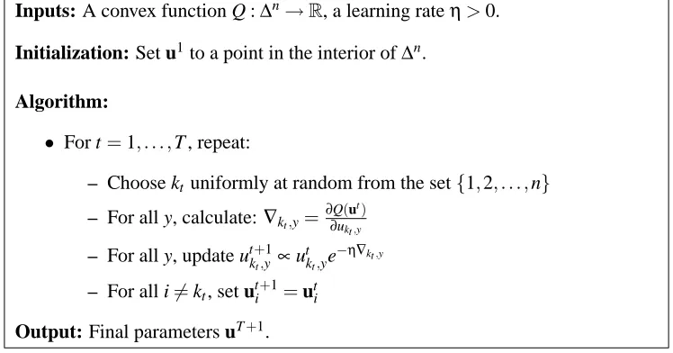
is typically very large, but labels can have useful internal structure. As one example, in CRFs each

Inputs: A convex function Q :∆n_{→R, a learning rate}η_>0.

Initialization: Set u1to a point in the interior of∆n.

Algorithm:

• For t=1, . . . ,T , repeat:

– For all i,y, calculate∇i,y=∂Q(u t₎ ∂ui,y – For all i,y, update ut_i,y+1∝ut_i,ye−η∇i,y Output: Final parameters uT+1.

Figure 1: A general batch EG Algorithm for minimizing Q(u) subject to u∈∆n_{. We use u}t _to

denote the set of parameters after t iterations.

Inputs: A convex function Q :∆n→R, a learning rateη>0.

Initialization: Set u1to a point in the interior of∆n.

Algorithm:

• For t=1, . . . ,T , repeat:

– Choose kt uniformly at random from the set{1,2, . . . ,n}

– For all y, calculate:∇kt,y=∂Q(u t₎ ∂ukt,y

– For all y, update ut_kt+_,y1∝ut_kt,ye−η∇kt,y – For all i6=kt, set ut_i+1=ut_i

Output: Final parameters uT+1.

Figure 2: A general randomized online EG Algorithm for minimizing Q(u)subject to u∈∆n_.

label y is an m-dimensional vector specifying the labeling of all m vertices in a graph. In parsing each label y is an entire parse tree. In both of these cases, the number of labels typically grows exponentially quickly with respect to the size of the inputs x.

We follow the framework for structured problems described by Bartlett et al. (2005). Each label y is defined to be a set of parts. We use R to refer to the set of all possible parts.5 We make the assumption that the feature vector for an entire label y decomposes into a sum over feature vectors for individual parts as follows:

f(x,y) =

∑

r∈y f(x,r).

Note that we have overloaded f to apply to either labels y or parts r.

As one example, consider a CRF which has an underlying graph with m nodes, and a maximum clique size of 2. Assume that each node can be labeled with one of two labels, 0 or 1. In this case the labeling of an entire graph is a vector y∈ {0,1}m_{. Each possible input x is usually a vector in}

X

m _{for some set}

X

_{, although this does not have to be the case. Each part corresponds to a tuple}

(u,v,yu,yv)where(u,v)is an edge in the graph, and yu,yv are the labels for the two vertices u and

v. The feature vector f(x,r) can then track any properties of the input x together with the labeled clique r= (u,v,yu,yv). In CRFs with clique size greater than 2, each part corresponds to a labeled

clique in the graph. In natural language parsing, each part can correspond to a context-free rule at a particular position in the sentence x (see Bartlett et al., 2005; Taskar et al., 2004b, for more details). The label set

Y

can be extremely large in structured prediction problems. For example, in a CRF with an underlying graph with m nodes and k possible labels at each node, there are kmpossible labelings of the entire graph. The algorithms we have presented so far require direct manipulation of dual variables ui,y corresponding to each possible labeling of each training example; they will

therefore be intractable in cases where there are an exponential number of possible labels. However, in this section we describe an approach that does allow an efficient implementation of the algorithms in several cases. The approach is based on the method originally described in Bartlett et al. (2005). The key idea is as follows. Instead of manipulating the dual variables ui for each i directly, we

will make use of alternative data structures si for all i. Each siis a vector of real values si,r for all

r∈R. In general we will assume that there are a tractable (polynomial) number of possible parts, and therefore that the number of si,r variables is also polynomial. For example, for a linear chain

CRF with m nodes and k labels at every node, each part takes the form r= (u,v,yu,yv), and there

are(m−1)k2_{possible parts.}

In the max-margin case, we follow Taskar et al. (2004a) and make the additional assumption that the error function decomposes into “local” error functions over parts:

e(xi,yi,y) =

∑

r∈y

e(xi,yi,r).

For example, when

Y

is a sequence of variables, the cost could be the Hamming distance between the correct sequence yiand the predicted sequence y; it is straightforward to decompose the

Ham-ming distance as a sum over parts as shown above. For brevity, in what follows we use ei,r instead

of e(xi,yi,r).

The sivariables are used to implicitly define regular dual values ui=p(si)where p :R|R|→∆

is defined as

py(s) =

exp

∑r∈ysr

∑y0exp∑_r∈y0s_r

.

To see how the sivariables can be updated, consider again the EG updates on the dual u variables.

The EG updates in all algorithms in this paper take the form

u0_i,y= ui,yexp{−η∇i,y}

∑yˆui,yˆexp{−η∇i,yˆ}

,

where for QLL

∇i,y=1+log ui,y+1

and for QMM,

∇i,y=−bi,y+

1

Cw(u)·(f(xi,yi)−f(xi,y)), where bi,y=e(xi,yi,y)as in Section 2.3.

Notice that, for both objective functions, the gradients can be expressed as a sum over parts. For the QLLobjective function, this follows from the fact that ui=p(si)and from the assumption that

the feature vector decomposes into parts. For the QMMobjective, it follows from the latter, and the

assumption that the loss decomposes into parts. The following lemma describes how EG updates on the u variables can be restated in terms of updates to the s variables, provided that the gradient decomposes into parts in this way.

Lemma 1 For a given u∈∆n_{, and for a given i∈[1. . .n], take u}0

i to be the updated value for ui

derived using an EG step, that is,

u0_i,y= ui,yexp{−η∇i,y}

∑yˆui,yˆexp{−η∇i,yˆ}

.

Suppose that, for some Giand gi,r, we can write∇i,y=Gi+∑r∈ygi,rfor all y. Then if ui=p(si)for

some si∈

R

|R|, and for all r we define

s0_i,r=si,r−ηgi,r,

it follows that u0_i=p(s0_i).

Proof: We show that, for ui=p(si), updating the si,ras described leads to p(s0i) =u0i. For suitable

partition functions Zi, Zi0, and Zi00, we can write

py(s0i) =

exp∑r∈y(si,r−ηgi,r)

Zi

= ui,yexp

−η∑r∈ygi,r

Z_i0

= ui,yexp{−η(∇i,y−Gi)}

Z_i0

= ui,yexp{−η∇i,y}

Z_i00

= u0_i,y.

In the case of the QLLobjective, a suitable update is

s0_i,r=si,r−η

si,r−

1

Cw(u)·f(xi,r)

.

In the case of the QMMobjective, a suitable update is

s0_i,r=si,r−η

−ei,r−1

Cw(u)·f(xi,r)

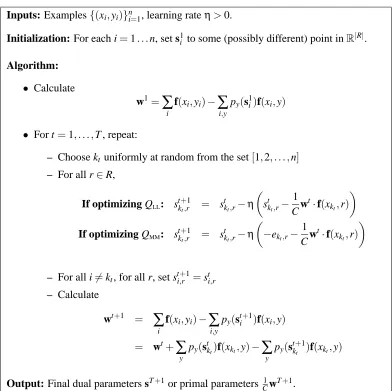
Inputs: Examples{(xi,yi)}ni=1, learning rateη>0.

Initialization: For each i=1. . .n, set s1_i to some (possibly different) point inR|R|.

Algorithm:

• Calculate

w1=

∑

i

f(xi,yi)−

∑

i,y

py(s1i)f(xi,y)

• For t=1, . . . ,T , repeat:

– Choose kt uniformly at random from the set[1,2, . . . ,n]

– For all r∈R,

If optimizing QLL: st_kt+_,r1 = st_kt,r−η

st_kt,r−1 Cw

t_·f(x kt,r)

If optimizing QMM: s

t+1

kt,r = stkt,r−η

−ekt,r−

1 Cw

t_·f(x kt,r)

– For all i6=kt, for all r, set sti,r+1=sti,r – Calculate

wt+1 =

∑

i

f(xi,yi)−

∑

i,y

py(sti+1)f(xi,y)

= wt+

∑

y

py(stkt)f(xkt,y)−

∑

y

py(st_kt+1)f(xkt,y)

Output: Final dual parameters sT+1or primal parameters_C1wT+1.

Figure 3: An implementation of the algorithm in Figure 2 using a part-based representation. The algorithm uses variables si for i=1. . .n as a replacement for the dual variables ui in

Figure 2.

Because of this result, all of the EG algorithms that we have presented can be restated in terms of the s variables: instead of maintaining a sequence ut={ut₁,ut₂, . . . ,ut_n}of dual variables, a sequence

st ={st₁,st₂, . . . ,st_n}is maintained and updated using the method described in the above lemmas.6

To illustrate this, Figure 3 gives a version of the randomized algorithm in Figure 2 that makes use of s variables. The batch algorithm can be implemented in a similar way.

The main computational challenge in the new algorithms comes in computing the parameter vector w(p(st)). The value for w(p(st))can be expressed as a function of the marginal probabilities of the part variables, as follows:

w(p(st)) =

∑

i

∑

y

ui,y(f(xi,yi)−f(xi,y))

=

∑

i

f(xi,yi)−

∑

i,y

py(sti)f(xi,y)

=

∑

i

f(xi,yi)−

∑

i,yr∈y

∑

py(sti)f(xi,r)

=

∑

i

f(xi,yi)−

∑

i r∈R

∑

µi,r(sti)f(xi,r).

Here the µi,rterms correspond to marginals, defined as

µi,r(sti) =

∑

y:r∈y

py(sti).

The mapping from parameters st_i to marginals µi,r(sti)can be computed efficiently in several

impor-tant cases of structured models. For example, in CRFs belief propagation can be used to efficiently calculate the marginal values, assuming that the tree-width of the underlying graph is small. In weighted context-free grammars the inside-outside algorithm can be used to calculate marginals, assuming that the set of parts R corresponds to context-free rule productions. Once marginals are computed, it is straightforward to compute w(p(st))and thereby implement the part-based EG al-gorithms.

5. Convergence Results

In this section, we provide convergence results for the EG batch and online algorithms presented in Section 3. Section 5.1 provides the key results, and the following sections give the proofs and the technical details.

5.1 Main Convergence Results

Our convergence results give bounds on how quickly the error|Q(u)−Q(u∗)|decreases with respect to the number of iterations, T , of the algorithms. In all cases we have|Q(u)−Q(u∗)| →0 as T→∞. In what follows we use D[pkq]to denote the KL divergence between p,q∈∆n_{(see Section 5.2).}

We also use|A|_∞to denote the maximum magnitude element of A (i.e.,|A|_∞=max(i,y),(j,z)|A(i,y),(j,z)|). The first theorem provides results for the EG-batch algorithms, and the second for the randomized online algorithms.

Theorem 1 For the batch algorithm in Figure 1, for QLLand QMM,

Q(u∗)≤Q(uT+1)≤Q(u∗) + 1

ηTD[u

∗_ku1_{], (6)}

assuming that the learning rate η satisfies 0<η≤ 1

1+n|A|∞ for QLL, and 0<η≤ _n|A|1_∞ for QMM.

Furthermore, for QLL,

Q(u∗)≤Q(uT+1)≤Q(u∗) +e

−ηT

Batch Algorithm

Online Algorithm

Q

MM

n2

ε

|

A

|∞

D

[

u

∗

k

u

1

]

nε

|

A

|∞

D

[

u

∗

k

u

1

] +

Q

(

u

1

)

−

Q

(

u

∗

)

Q

LL

n

(

1

+

n

|

A

|

∞

)

log

(

c1

ε

)

n

(

1

+

|

A

|

∞

)

log

(

cε2

)

Table 1: Each entry shows the amount of computation (measured in terms of the number of training sample processed using the EG updates) required to obtain |Q(u)−Q(u∗)| ≤ε for the batch algorithm, or E[|Q(u)−Q(u∗)|]≤εfor the online algorithm, for a givenε>0. The constants are c1= (1+n|A|∞)D[u∗ku1], and c2=

(1+|A|_∞)D[u∗ku1] +Q(u1)−Q(u∗))

.

assuming again that 0<η≤ 1 1+n|A|∞.

The randomized online algorithm will produce different results at every run, since different points will be processed on different runs. Our main result for this algorithm characterizes the mean value of the objective Q(uT+1)when averaged over all possible random orderings of points. The result implies that this mean will converge to the optimal value Q(u∗).

Theorem 2 For the randomized algorithm in Figure 2, for QLLand QMM,

Q(u∗)≤EQ(uT+1)

≤Q(u∗) + n

ηTD[u

∗_ku1_{] +}n T

Q(u1)−Q(u∗)

, (7)

assuming that the learning rate η satisfies 0<η≤ 1

1+|A|∞ for QLL, and 0<η≤ _|A|1_∞ for QMM.

Furthermore, for QLL, for the algorithm in Figure 2,

Q(u∗)≤EQ(uT+1)

≤Q(u∗) +e−ηnT

1

ηD[u∗ku1] +Q(u1)−Q(u∗)

,

assuming again that 0<η≤ 1 1+|A|∞.

The above result characterizes the average behavior of the randomized algorithm, but does not provide guarantees for any specific run of the algorithm. However, by applying the standard ap-proach of repeated sampling (see, for example, Mitzenmacher and Upfal, 2005; Shalev-Shwartz et al., 2007), one can obtain a solution that, with high probability, does not deviate by much from the average behavior. In what follows, we briefly outline this derivation.

Note that the random variable Q(uT+1)−Q(u∗)is nonnegative, and so by Markov’s inequality, it satisfies

Pr

n

Q(uT+1)−Q(u∗)≥2 EQ(uT+1)

−Q(u∗)o

≤1 2 .

Given some δ>0, if we run the algorithm k=log₂(1

δ) times,7 each time with T iterations, and

choose the best ˆu of these k results, we see that

Pr

n

Q(ˆu)−Q(u∗)≥2 EQ(uT+1)

−Q(u∗)o

≤δ.

7. Assume for simplicity that log₂(1

Thus, for any desired confidence 1−δ, we can obtain a solution that is within a factor of 2 of the bound for T iterations in Theorem 2 by using T log₂(1_δ) iterations. In our experiments, we found that repeated trials of the randomized algorithm did not yield significantly different results.

The first consequence of the two theorems above is that the batch and randomized online algo-rithms converge to a u with the optimal value Q(u∗). This follows since Equations 6 and 7 imply that as T →∞the value of Q(uT+1)approaches Q(u∗).

The second consequence is that for a givenε>0 we can find the number of iterations needed to reach a u such that|Q(u)−Q(u∗)| ≤εfor the batch algorithm or E[|Q(u)−Q(u∗)|]≤εfor the online algorithm. Table 1 shows the computation required by the different algorithms, where the computation is measured by the number of training examples that need to be processed using the EG updates.8 The entries in the table assume that the maximum possible learning rates are used for each of the algorithms—that is, _1+n|A|1

∞ for LLEG-Batch,

1

1+|A|∞ for LLEG-Online,

1

n|A|∞ for

MMEG-batch, and _|A|1

∞ for MMEG-Online.

Crucially, note that these rates suggest that the online algorithms are significantly more efficient than the batch algorithms; specifically, the bounds suggest that the online algorithms require a factor of n less computation in both the QLLand QMMcases. Thus these results suggest that the randomized

online algorithm should converge much faster than the batch algorithm. Roughly speaking, this is a direct consequence of the learning rateη being a factor of n larger in the online case (see also Section 9). This prediction is confirmed in our empirical evaluations, which show that the online algorithm is far more efficient than the batch algorithm.

A second important point is that the rates for QLLlead to an O(log(1ε))dependence on the desired

accuracyε, which is a significant improvement over QMM, which has an O(1ε)dependence. Note that

the O(1

ε)dependence for QMMis similar to several other max-margin algorithms in the literature (see

Section 6 for more discussion).

To gain further intuition into the order of magnitude of iterations required, note that the factor D[u∗ku1]which appears in the above expressions is at most n log|

Y

|, which can be achieved by setting u1_i to be the uniform distribution over

Y

for all i. Also, the value of|A|_∞can easily be seen to be _C1maxi,ykgi,yk2.

In the remainder of this section we give proofs of the results in Theorems 1 and 2. In doing so, we also give theorems that apply to the optimization of general convex functions Q :∆n→R.

5.2 Divergence Measures

Before providing convergence proofs, we define several divergence measures between distributions. Define the KL divergence between two distributions ui,vi∈∆to be

D[uikvi] =

∑

y

ui,ylog

ui,y

vi,y .

Given two sets of n distributions u,v∈∆n_{define their KL divergence as}

D[ukv] =

∑

i

D[uikvi].

Next, we consider a more general class of divergence measures, Bregman divergences (e.g., see Bregman, 1967; Censor and Zenios, 1997; Kivinen and Warmuth, 1997). Given a convex function Q(u), the Bregman divergence between u and v is defined as

BQ[ukv] =Q(u)−Q(v)−∇Q(v)·(u−v).

Convexity of Q implies BQ[ukv]≥0 for all u,v∈∆n.

Note that the Bregman divergence with Q(u) =∑_i,yui,ylog ui,y is the KL divergence. We shall

also be interested in the Mahalanobis distance

MA[ukv] =

1 2(u−v)

T_A(u−v),

which is the Bregman divergence for Q(u) =1 2u

T_Au.

In what follows, we also use the Lpnorm defined for x∈Rmaskxkp= p p

∑i|xi|p.

5.3 Dual Improvement and Bregman Divergence

In this section we provide a useful lemma that determines when the EG updates in the batch al-gorithm will result in monotone improvement of Q(u). The lemma requires a condition on the relation between the Bregman and KL divergences which we define as follows (the second part of the definition will be used in the next section):

Definition 5.1 : A convex function Q :∆n _{→R is} τ_{-upper-bounded for some} τ_{>0 if for any} p,q∈∆n_,

BQ[pkq]≤τD[pkq].

In addition, we say Q(u)is(µ,τ)-bounded for constants 0<µ<τif for any p,q∈∆n_,

µD[pkq]≤BQ[pkq]≤τD[pkq].

The next lemma states that if Q(u)isτ-upper-bounded, then the change in the objective as a result of an EG update can be related to the KL divergence between consecutive values of the dual variables.

Lemma 2 If Q(u)isτ-upper-bounded, then ifηis chosen such that 0<η≤ 1_τ, it holds that for all t in the batch algorithm (Figure 1):

Q(ut)−Q(ut+1)≥ 1

ηD[utkut+1].

Proof: Given a ut, the EG update is

ut_i,y+1= 1

Zt i

ut_i,ye−η∇ti,y ,

where

∇t

i,y=

∂Q(ut)

∂ui,y

, Z_it=

∑

ˆ

y

Simple algebra yields

∑

i

D[ut_ikut_i+1] +D[ut_i+1kut_i]

=η

∑

i,y

(ut_i,y−ut_i,y+1)∇t i,y.

Equivalently, using the notation for KL divergence between multiple distributions:

D[utkut+1] +D[ut+1kut] =η(ut−ut+1)·∇Q(ut).

The definition of the Bregman divergence BQthen implies

−ηBQ[ut+1kut] +D[utkut+1] +D[ut+1kut] =η(Q(ut)−Q(ut+1)). (8)

Since Q(u)isτ-upper-bounded andη≤1_τ it follows that D[ut+1kut]≥ηBQ[ut+1kut], and together

with Eq. 8 we obtain the desired resultη(Q(ut)−Q(ut+1))≥D[utkut+1].

Note that the condition in the lemma may be weakened to requiring that τD[utkut+1]≥ BQ[utkut+1]for all t. For simplicity, we require the condition for all p,q∈∆n. Note also that

D[pkq]≥0 for all p,q∈∆n_{, so the lemma implies that for an appropriately chosen}η_{, the EG}

up-dates always decrease the objective Q(u). We next show that the log-linear dual QLL(u)is in fact τ-upper-bounded.

Lemma 3 Define |A|_∞ to be the maximum magnitude of any element of A, that is, |A|_∞ =

max(i,y),(j,z)|A(i,y),(j,z)|. Then QLL(u)isτLL-upper-bounded withτLL=1+n|A|∞.

Proof: First notice that the Bregman divergence BQis linear in Q. Thus, for any p,q∈∆n we can

write BQLL as a sum of two terms (see Eq. 4).

BQLL[pkq] =D[pkq] +MA[pkq].

We first bound MA[pkq]in terms of squared L1distance between p and q. Denote r=p−q. Then: MA[pkq] =

1

2_i,y,

∑

_j,zri,yrj,zA(i,y),(j,z)≤ |A|∞

2 _i,y,

∑

_j,z|ri,y||rj,z|= |A|∞

2 kp−qk 2 1.

Next, we use the inequality D[p1kp2]≥₂1kp1−p2k21(also known as Pinsker’s inequality, see Cover and Thomas, 1991, p. 300), which holds for any two distributions p1 and p2. Consider the two distributions ˆp=1_np and ˆq=1_nq, each defined over an alphabet of size n|

Y

|. Then it follows that:9

|A|_∞

2 kp−qk 2 1=

n2|A|_∞

2 kˆp−ˆqk 2

1≤n2|A|∞D[ˆpkˆq] =n|A|∞D[pkq], and thus MA[pkq]≤n|A|∞D[pkq]. So for the Bregman divergence of QLL(u)we obtain

BQLL[pkq]≤(1+n|A|∞)D[pkq],

yielding the desired result.

The next lemma shows that a similar result can be obtained for the QMMobjective.

Lemma 4 The function QMM(u)isτMM-upper-bounded withτMM=n|A|∞.

Proof: For QMMdefined in Eq. 5, we have

BQMM[pkq] =MA[pkq].

We can then use a similar derivation to that of Lemma 3 to obtain the result.

We thus have that the condition in Lemma 2 is satisfied for both the QLL(u)and QMM(u)

objec-tives, implying that their EG updates result in monotone improvement of the objective, for a suitably chosenη:

Corollary 1 The LLEG-Batch algorithm with 0<η≤_τ1

LL satisfies for all t

QLL(ut)−QLL(ut+1)≥

1

ηD[utkut+1],

and the MMEG-Batch algorithm with 0<η≤ 1

τMM satisfies for all t

QMM(ut)−QMM(ut+1)≥

1

ηD[utkut+1].

5.4 Convergence Rates for the EG Batch Algorithms

The previous section showed that for appropriate choices of the learning rateη, the batch EG updates are guaranteed to improve the QLLand QMMloss functions at each iteration. In this section we build

directly on these results, and address the following question: how many iterations does the batch EG algorithm require so that the|Q(ut)−Q(u)| ≤εfor a given ε>0? We show that as long as Q(u)isτ-upper-bounded, the number of iterations required is O(1

ε). This bound thus holds for both

the log-linear and max-margin batch algorithms. Next, we show that if Q(u)is(µ,τ)-bounded, the rate can be significantly improved to requiring O(log(1

ε))iterations. We conclude by showing that

QLL(u)is(µ,τ)-bounded, implying that the O(log(1ε))rate holds for LLEG-Batch.

The following result gives an O(1_ε)rate for QLLand QMM:

Lemma 5 If Q(u) is τ-upper-bounded and 0≤η≤ 1

τ, then after T iterations of the EG-Batch

algorithm, for any z∈∆n_{including z=u}∗_,

Q(uT+1)−Q(z)≤ 1

ηTD[zku 1_].

Proof: See Appendix A.

The lemma implies that to get ε-close to the optimal objective value, O(1

ε) iterations are

required—more precisely, if a choice of η= 1_τ is made, then at most τ_εD[zku1]iterations are re-quired. Since its conditions are satisfied by both QLL(u)and QMM(u)(given an appropriate choice

ofη) the result holds for both the LLEG-Batch and MMEG-Batch algorithms.

Lemma 6 If Q(u)is(µ,τ)-bounded and 0<η≤ 1

τ then after T iterations of the EG-Batch

algo-rithm, for any z∈∆n_{including z=u}∗_,

Q(uT+1)−Q(z)≤e

−ηµT

η D[z||u1].

Proof: See Appendix B.

The lemma implies that an accuracy ofεmay be achieved by using O(log(1

ε))iterations.

To see why QLL(u)is(µ,τ)-bounded note that for any p,q∈∆n,

BQLL[pkq] =D[pkq] +MA[pkq]≥D[pkq],

implying (together with Lemma 3) that QLL(u)is(1,τLL)-bounded.

Finally, note that Lemmas 5 and 6, together with the facts that QLLis(1,τLL)-bounded and QMM

isτMM-upper-bounded, imply Theorem 1 of Section 5.1.

5.5 Convergence Results for the Randomized Online Algorithm

This section analyzes the rate of convergence of the randomized online algorithm in Figure 2. Before stating the results, we need some definitions. We will use Qu,i:∆→Rto be the function defined as

Qu,i(v) =Q(u1,u2, . . . ,ui−1,v,ui+1, . . . ,un),

for any v∈∆. We denote the Bregman divergence associated with Qu,i as BQu,i[xky]. We then

introduce the following definitions:

Definition 5.2 : A convex function Q :∆n→Risτ-online-upper-bounded for someτ>0 if for any

i∈1. . .n and for any p,q∈∆,

BQu,i[pkq]≤τD[pkq].

In addition, Q is(µ,τ)-online-bounded for 0<µ<τif Q isτ-online-upper-bounded, and in addition, for any p,q∈∆n_,

µD[pkq]≤BQ[pkq].

Note that the lower bound in the above definition refers to BQand not to BQu,i. Also, note that if a

function is(µ,τ)-online-bounded then it must also beτ-online-upper-bounded. The following lemma then gives results for the QLLand QMMfunctions:

Lemma 7 The log-linear dual QLL(u) is (µ,τ)-online-bounded for µ=1 and τ=1+|A|∞. The

max-margin dual QMM(u)isτ-online-upper-bounded forτ=|A|∞.

Proof: See Appendix C.

Lemma 8 Consider the algorithm in Figure 2 applied to a convex function Q(u)that isτ -online-upper-bounded. Ifη>0 is chosen such thatη≤1_τ, then it follows that for all z∈∆n

EQ(uT+1)

≤Q(z) + n

ηTD[zku 1_{] +}n

T

Q(u1)−Q(u∗) ,

where EQ(uT+1)

is the expected value of Q(uT+1), and u∗=argmin_u∈∆nQ(u). Proof: See Appendix D.

The previous lemma shows, in particular, that the online EG algorithm converges at an O(1_ε)

rate for the function QMM. However, we can prove a faster rate of convergence for QLL, which is

(µ,τ)-online-bounded. The following lemma shows that such functions exhibit an O(log(1

ε))rate of

convergence.

Lemma 9 Consider the algorithm in Figure 2 applied to a convex function Q(u) that is(µ,τ) -online-bounded. Ifη>0 is chosen such thatη≤1

τ, then it follows that for all z∈∆n

E

Q(uT+1)

≤Q(z) +e−ηµTn

1

ηD[zku1] +Q(u1)−Q(u∗)

,

where u∗=argmin_u∈∆nQ(u).

Proof: See Appendix E.

Note that Lemmas 7, 9 and 8 complete the proof of Theorem 2 in Section 5.1.

6. Related Work

The idea of solving regularized loss-minimization problems via their convex duals has been ad-dressed in several previous papers. Here we review those, specifically focusing on the log-linear and max-margin problems.

Zhang (2002) presented a study of convex duals of general regularized loss functions, and pro-vided a methodology for deriving such duals. He also considered a general procedure for solving such duals by optimizing one coordinate at a time. However, it is not clear how to implement this procedure in the structured learning case (i.e., when |

Y

|is large), and convergence rates are not given.

In the specific context of log-linear models, several papers have addressed dual optimization. Earlier work (Jaakkola and Haussler, 1999; Keerthi et al., 2005; Zhu and Hastie, 2001) treated the logistic regression model, a simpler version of a CRF. In the binary logistic regression case, there is essentially one parameter uiper example with the constraint 0≤ui≤1, and therefore simple

line-search methods can be used for optimization. Minka (2003) presents empirical results which show that this approach performs similarly to conjugate gradient. The problem becomes much harder when uiis constrained to be a distribution over many labels, as in the case discussed here. Recently,

Memisevic (2006) addressed this setting, and suggests optimizing ui by transferring probability

While some previous work on log-linear models proved convergence of dual methods (e.g., Keerthi et al., 2005), we are not aware of rates of convergence that have been reported in this context. Convergence rates for related algorithms, in particular a generalization of EG, known as the Mirror-Descent algorithm, have been studied in a more general context in the optimization literature. For instance, Beck and Teboulle (2003) describe convergence results which apply to quite general definitions of Q(u), but which have only O(1

ε2) convergence rates, as compared to

our results of O(1_ε)and O(log(1_ε))for the max-margin and log-linear cases respectively. Also, their work considers optimization over a single simplex, and does not consider online-like algorithms such as the one we have presented.

For max-margin models, numerous dual methods have been suggested, an earlier example being the SMO algorithm of Platt (1998). Such methods optimize subsets of the u parameters in the dual SVM formulation (see also Crammer and Singer, 2002). Analysis of a similar algorithm (Hush et al., 2006) results in an O(1

ε)rate, similar to the one we have here. Another algorithm for solving

SVMs via the dual is the multiplicative update method of Sha et al. (2007). These updates are shown to converge to the optimum of the SVM dual, but convergence rate has not been analyzed, and extension to the structured case seems non-trivial. An application of EG to binary SVMs was previously studied by Cristianini et al. (1998). They show convergence rates of O(1

ε2), that are

slower than our O(1_ε), and no extension to structured learning (or multi-class) is discussed.

Recently, several new algorithms have been presented, along with a rate of convergence analysis (Joachims, 2006; Shalev-Shwartz et al., 2007; Teo et al., 2007; Tsochantaridis et al., 2004; Taskar et al., 2006). All of these algorithms are similar to ours in having a relatively low dependence on n in terms of memory and computation. Among these, Shalev-Shwartz et al. (2007), Teo et al. (2007) and Taskar et al. (2006) present an O(1_ε)rate, but where accuracy is measured in the primal or via the duality gap, and not in the dual as in our analysis. Thus, it seems that a rate of O(1

ε)is currently

the best known result for algorithms that have a relatively low dependence on n (general QP solvers, which may have O(log(1_ε)) behavior, generally have a larger dependence on n, both in time and space). Note that, as in our analysis, all these convergence rates depend on|A|_∞.

Finally, we emphasize again that the EG algorithm is substantially different from stochastic gradient and stochastic subgradient approaches (LeCun et al., 1998; Nedic and Bertsekas, 2001; Shalev-Shwartz et al., 2007; Vishwanathan et al., 2006). EG and stochastic gradient methods are similar in that they both process a single training example at a time. However, EG corresponds to block-coordinate descent in the dual, and uses the exact gradient with respect to the block being updated. In contrast, stochastic gradient methods directly optimize the primal problem, and at each update use a single example to approximate the gradient (or subgradient) of the primal objective function.

7. Experiments on Regularized Log-Likelihood

its performance to L-BFGS (Byrd et al., 1995), which is a batch gradient descent method, and to stochastic gradient descent.10

We do not report results on LLEG-Batch, since we found it to converge much more slowly than the online algorithm. This is expected from our theoretical results, which anticipate a factor of n speed-up for the online algorithm. We also report experiments comparing the randomized online algorithm to a deterministic online EG algorithm, where samples are drawn in a fixed order (e.g., the algorithm first visits the first example, then the second, etc.).

Although EG is guaranteed to converge for an appropriately chosenη, it turns out to be bene-ficial to use an adaptive learning rate. Here we use the following simple strategy: we first consider only 10% of the data-set, and find a value ofηthat results in monotone improvement for at least 95% of the samples. Denote this value byηini _{(for the experiments in Section 7.1 we simply use} ηini_{=0.5). For learning over the entire data-set, we keep a learning rate}η

ifor each sample i (where

i=1, . . . ,n), and initialize this rate toηini _{for all points. When sample i is visited, we halve}η

iuntil

an improvement in the objective is obtained. Finally, after the update, we multiplyηi by 1.05, so

that it does not decrease monotonically.

It is important that when updating a single example using the online algorithms, the improve-ment (or decrease) in the dual can be easily evaluated, allowing the halving strategy described in the previous paragraph to be implemented efficiently. If the current dual parameters are u, the i’th coordinate is selected, and the EG updates then map ui to u0i, the change in the dual objective is

∑

y

u0_i,ylog u0_i,y+ 1

2C

w(u) +

∑

y

u0_i,y−ui,ygi,y

2 −

∑

y

ui,ylog ui,y− 1

2Ckw(u)k 2

.

The primal parameters w(u) are maintained throughout the algorithm (see Figure 3), so that this change in the dual objective can be calculated efficiently. A similar method can be used to calculate the change in the dual objective in the max-margin case.

We measure the performance of each training algorithm (the EG algorithms, as well as the batch gradient and stochastic gradient methods) as a function of the amount of computation spent. Specifically, we measure computation in terms of the number of times each training example is visited. For EG, an example is considered to be visited for every value ofηthat is tested on it. For L-BFGS, all examples are visited for every evaluation performed by the line-search routine. We define the measure of effective iterations to be the number of examples visited, divided by n. In the following sections we compare the algorithms in terms of their performance as a function of the effective number of iterations. A comparison in terms of running time is provided in Appendix F; there is little difference between the timed comparisons and the results presented in this section.

7.1 Multi-class Classification

We first conducted multi-class classification experiments on the MNIST classification task. Exam-ples in this data set are images of handwritten digits represented as 784-dimensional vectors. We used a training set of 59k examples, and a validation set of 10k examples.11 Note that since we 10. We also experimented with conjugate gradient algorithms, but since these resulted in worse performance than

L-BFGS, we do not report these results here.

only use a linear kernel, accuracy results are not competitive with state of the art classifiers which use non-linear kernels (e.g., see Cortes and Vapnik, 1995). We define a ten-class logistic-regression model where

p(y|x)∝ex·wy ,

and x,wy∈R784,y∈ {1, . . . ,10}.

Models were trained for various values of the regularization parameter C: specifically, we tried values of C equal to 1000, 100, 10, 1, 0.1, and 0.01. Convergence of the EG algorithm for low values of C (i.e., 0.1 and 0.01) was found to be slow; we discuss this issue more in Section 7.1.1, arguing that it is not a serious problem.

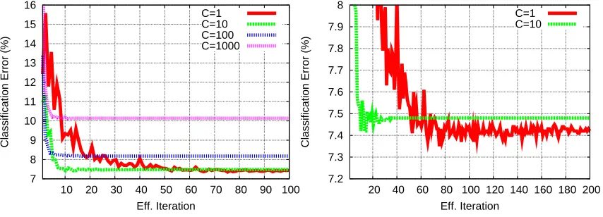
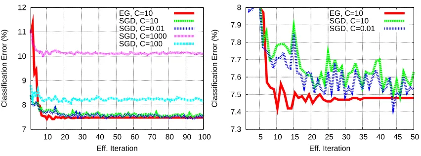
Figure 4 shows plots of the validation error versus computation for C equal to 1000, 100, 10, and 1, when using the EG algorithm. For C equal to 10 or more, convergence is fast. For C=1 convergence is somewhat slower. Note that there is little to choose between C=10 and C=1 in terms of validation error.

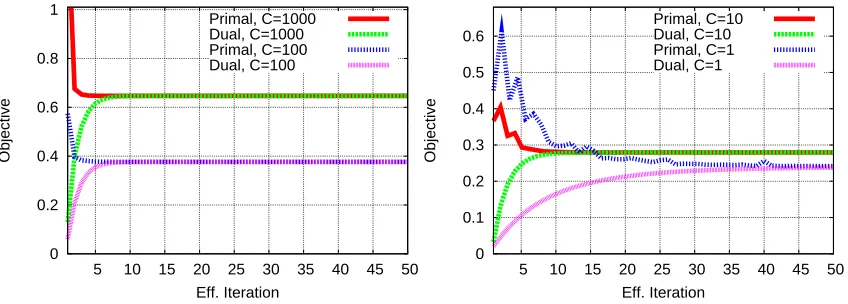
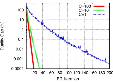
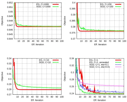
Figure 5 shows plots of the primal and dual objective functions for different values of C. To obtain the primal objective values, we used the EG weight vector _C1w(ut). Note that EG does not explicitly minimize the primal objective function, so the EG primal will not necessarily decrease at every iteration. Nevertheless, our experiments show that the EG primal decreases quite quickly. Figure 6 shows how the duality gap decreases with the amount of computation spent (the duality gap is the difference between the primal and dual values at each iteration). The log of the duality gap decreases more-or-less linearly with the amount of computation spent, as predicted by the O(log(1

ε))

bounds on the rate of convergence.12

Finally, we compare the deterministic and randomized versions of the EG algorithm. Figure 7 shows the primal and dual objectives for both algorithms. It can be seen that the randomized algo-rithm is clearly much faster to converge. This is even more evident when plotting the duality gap, which converges much faster to zero in the case of the randomized algorithm. These results give empirical evidence that the randomized strategy is to be preferred over a fixed ordering of the train-ing examples (note that we have been able to prove bounds on convergence rate for the randomized algorithm, but have not been able to prove similar bounds for the deterministic case).

7.1.1 CONVERGENCE FORLOWVALUES OFC

As mentioned in the previous section, convergence of the EG algorithm for low values of C can be very slow. This is to be expected from the bounds on convergence, which predict that convergence time should scale linearly with _C1 (other algorithms, e.g., see Shalev-Shwartz et al., 2007, also require O(1

C)time for convergence). This is however, not a serious problem on the MNIST data,

where validation error has reached a minimum point for around C=10 or C=1.

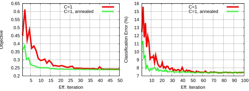
If convergence for small values of C is required, one strategy we have found effective is to start C at a higher value, then “anneal” it towards the target value. For example, see Figure 8 for results for C=1 using one such annealing scheme. For this experiment, if we take t to be the number of iterations over the training set, where for any t we have processed t×n training examples, we set C=10 for t≤5, and set C=1+9×0.7t−5for t>5. Thus C starts at 10, then decays exponentially quickly towards the target value of 1. It can be seen that convergence is significantly faster for the annealed method. The intuition behind this method is that the solution to the dual problem for

7 8 9 10 11 12 13 14 15 16

10 20 30 40 50 60 70 80 90 100

Classification Error (%)

Eff. Iteration C=1 C=10 C=100 C=1000

7.2 7.3 7.4 7.5 7.6 7.7 7.8 7.9 8

20 40 60 80 100 120 140 160 180 200

Classification Error (%)

Eff. Iteration C=1 C=10

Figure 4: Validation error results on the MNIST learning task for log-linear models trained using the EG randomized online algorithm. The X axis shows the number of effective iterations over the entire data set. The Y axis shows validation error percentages. The left figure shows plots for values of C equal to 1, 10, 100, and 1000. The right figure shows plots for C equal to 1 and 10 at a larger scale.

C=10 is a reasonable approximation to the solution for C=1, and is considerably easier to solve; in the annealing strategy we start with an easier problem and then gradually move towards the harder problem of C=1.

7.1.2 ANEFFICIENTMETHOD FOROPTIMIZING ARANGE OFC VALUES

In practice, when estimating parameters using either regularized log-likelihood or hinge-loss, a range of values for C are tested, with cross-validation or validation on a held-out set being used to choose the optimal value of C. In the previously described experiments, we independently optimized log-likelihood-based models for different values of C. In this section we describe a highly efficient method for training a sequence of models for a range of values of C.

The method is as follows. We pick some maximum value for C; as in our previous experiments, we will choose a maximum value of C=1000. We also pick a tolerance valueε, and a parameter 0<v<1. We then optimize C using the randomized online algorithm, until the duality gap is less thanε×p, where p is the primal value. Once the duality gap has converged to within this ε tolerance, we reduce C by a factor of v, and again optimize to within anεtolerance. We continue this strategy—for each value of C optimizing to within a factor ofε, then reducing C by a factor of v—until C has reached a low enough value. At the end of the sequence, this method recovers a series of models for different values of C, each optimized to within a tolerance ofε.