A New Method on Solving Intuitionistic Fuzzy Transportation Problem

Vol. 15, No. 2, 2017, 163-171

ISSN: 2279-087X (P), 2279-0888(online) Published on 11 December 2017

www.researchmathsci.org

DOI: http://dx.doi.org/10.22457/apam.v15n2a2

163

Annals of

A New Method on Solving Intuitionistic Fuzzy

Transportation Problem

A.Nagoor Gani1 and S.Abbas2

1

PG & Research Department of Mathematics, Jamal Mohamed College Tiruchirappalli, Tamilnadu, India. e-mail: [email protected]

2

PG& Research Department of Mathematics, Khadir Mohideen College Adirampattinam, Tamilnadu, India. e-mail: [email protected]

Received 1 November 2017; accepted 9 December 2017

Abstract. In this paper, we find the optimum solution for an triangular intuitionistic fuzzy transportation problem using monalisha’s approximation method. Using this method we could get the optimum solution directly. An illustrative numerical example was given. Keywords: Intuitionistic Fuzzy Transportation Problem, Triangular Intuitionistic Fuzzy Number

AMS Mathematics Subject Classification (2010): 03E72, 90B06, 03F55 1. Introduction

Transportation Problem (TP) is based on supply and demand of commodities transported from several sources to the different destinations. The sources from which we need to transport refer the supply while the destination where commodities arrive referred the demand. It has been seen that on many occasion, the decision problem can also be formatting as TP. In general we try to minimize total transportation cost for the commodities transporting from source to destination.

A Fuzzy Transportation Problem (FTP) is a Transportation Problem (TP) in which the supply and demand are fuzzy quantities. The objective of the FTP is to determine the shipping schedule that minimizes the total fuzzy transportation cost while satisfying fuzzy supply and fuzzy demand. In [5], Nagoor Gani et al. presented a two stage cost minimizing fuzzy transportation problem in which supplies and demands are trapezoidal fuzzy numbers.

The concept of Intuitionistic Fuzzy Sets (IFSs) proposed by Atanassov[1] in 1986 is found to be highly useful to deal with vagueness. The major advantage of IFS over fuzzy set is that IFSs separate the degree of membership (belongingness) and the degree of non-membership (non–belongingness) of an element in the set. In [3], Nagoor Gani et al. Solving Intuitionistic Fuzzy Transportation Problem Using Zero Suffix Algorithm.

164

Transportation Problem(IFTP) is explained in Section 4.In Section 5, Monalisha’s Approximation Method is introduced and the steps are explained. A Numerical Example is illustrated in Section 6.

2. Preliminaries

Definition 2.1. Intuitionistic Fuzzy Set (IFS)

An Intuitionistic fuzzy set (IFS)

A

~

Iin X is given by a set of ordered triples :

I

A

~

= {<x,

µ

_A~I(x),

ν

_A~I(x)>/x∈X},

where

µ

_A~I,

ν

_A~I :X[0,1] are functions such that 0 ≤

µ

_A~I(x) +

ν

_A~I(x) ≤ 1 for all x ∈

X. For each x the numbers I

A~

µ

(x) and I

A~

ν

(x) represent the degree of membership and degree of non-membership of the element x∈X to A⊂ X, respectively.

Definition 2.2. Intuitionistic Fuzzy Number (IFN)

An intuitionistic fuzzy subset

A

~

I={<x,

µ

_A~I (x),

ν

_A~I(x)>/x∈X}, of the real line R is called an Intuitionistic Fuzzy Number (IFN) if the following holds:

i) There exist m∈R,

µ

_A~I (m)=1 and

ν

_A~I (m) =0.

ii) µA is a continuous mapping from R to the closed interval [ 0,1 ] and ∀ x∈R,

the relation 0≤

µ

_A~I(x) +

ν

_A~I(x ) ≤ 1 holds.

The membership and non-membership function of

A

~

I is of the following form:

0 for - ∝< x ≤ m-α f1(x) for x ∈[ m-α , m]

I A~

µ

(x) = 1 for x = m

h1(x) for x ∈ [m , m+β]

0 for m + β≤ x <∝

where f1(x) and h1(x) are strictly increasing and decreasing function in [ m-α , m] and

[m,m+β] respectively.

1 for - ∝< x ≤ m-α′

f2(x) for x ∈[ m-α′ , m] ; 0 ≤ f1(x)+f2(x) ≤ 1

ν

A~I (x) = 0 for x = m

h2(x) for x ∈ [m , m+β′] ; 0 ≤ h1(x) + h2(x) ≤ 1

165

Here m is the mean value of

A

~

I. α and β are called left and right spreads of membership function

µ

_A~I (x) respectively. α′ and β′ represents left and right spreads of

non membership function

ν

_A~I (x ) respectively. Symbolically, the intuitionistic fuzzy

number is represented as

A

~

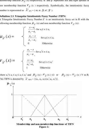
IIFN = ( m; α , β; α’, β’ ).

Definition 2.3. Triangular Intuitionistic Fuzzy Number (TIFN) A Triangular Intuitionistic Fuzzy Number I

A~ is an intuitionistic fuzzy set in R with the following membership function I

A

~

µ

(x) and non membership function I

A~

ν

(x): 1 2 1 a a a x − −

for a1≤ x ≤ a2

=

)

(

~I

x

A

µ

2 3 3 a a x a − −

for a2≤ x ≤ a3

0 Otherwise

' 1 2 2 a a x a − −

for a1′≤ x ≤ a2

=

)

(

~I

x

A

ν

2 3 2 ' a a a x − −

for a2≤ x ≤ a3′

1 Otherwise

where a1′≤ a1 ≤ a2 ≤ a3 ≤ a3′ and

µ

_A~I (x) +

ν

_A~I(x ) ≤1 or

µ

_A~I(x) =

ν

_A~I(x ) ∀ x∈R. This TIFN is denoted by _A~I

TIFN = {(a1, a2, a3);(a1′,a2, a3′)}.

166 Definition 2.4. Accuracy Function

We define

8

) 2

( ) 2

( ) ~

(A a1 a2 a3 a1 a2 a3 H I = + + + ′+ + ′ ,

an accuracy function of _A~I_{, to defuzzify the given number.}

3. Arithmetic operations of triangular intuitionistic fuzzy number

Let a~ = {(aI 1,a2,a3);(a1′,a2,a3′)} and I

b

~

= {(b1,b2,b3);(b1′, b2, b3′)} two triangular

Intuitionistic fuzzy number then the arithmetic operations on _a~ and I

_b

~

I _{as follows :}

Addition : I

a

~ _⊕ I

b

~

= ( a1+ b1, a2+b2, a3+b3)(a1′+b1′, a2+b2, a3′+b3′)

Subtraction : a~I

Θ

b

~

I=( a1-b3, a2-b2, a3-b1)( a1′-b3′, a2-b2, a3′-b1′)

Multiplication: a~I⊗

b

~

I = ( a1b1, a2b2, a3b3)(a1′b1′, a2b2, a3′b3′)

Scalar Multiplication : (i) If k>0 then k_a~ = (kaI

1,ka2,ka3)(ka1′,ka2,ka3′)

(ii) If k<0 then k I

a~ = (ka3,ka2,ka1)(ka3′,ka2,ka1′)

4. Intuitionistic fuzzy transportation problem (IFTP)

Consider a transportation with m Intuitionistic Fuzzy (IF) origins and n IF destination. Let Cij(i=1,2,…,m, j=1,2,…,n) be the cost of transporting one unit of the product form i

th

origin to jth destination .Let _a~I

i (i=1,2,…,m) be the quantity of commodity available at

IF origin i . Let

b

~

Ij (j=1,2,…,n) be the quantity of commodity needed of IF

destination j . Let Xij (i=1,2,…,m, j=1,2,…,n) is quantity transported from i th

IF origin to jth destination.

Mathematical Model of Intuitionistic Fuzzy Transportation Problem is

= ∑ ∑ ̃

= , = 1,2, … ,

= , = 1,2, … , ≥ 0 for all i and j

167

D1 D2 ⋯ Dn

IF Capacity

O1 C11 X11

C12 X12

⋯ C1n X1n

I

a~ 1 O2 C21

X21 C22 X22

⋯ C2n X2n

I

a~ 2

⋮ ⋮ ⋮

Om Cm1 Xm1

Cm2 Xm2

Cmn Xmn

I

a~ m IF

Demand

I

b

~

1

I

b

~

2

I

b

~

n

5. Monalisha's approximation method (MAM's) model Step 1: Determine the cost table from the given problem.

(i) Examine whether total demand equals total demand. If yes, go to step 2. (ii) If not, introduce a dummy row/column having all its cost elements as zero and supply/ demand as the (+ve) difference of supply and demand.

Step 2: Locate the smallest element in each row of the given cost matrix and then subtract the same from each element of that row.

Step 3: In the reduced matrix obtained in step 2, locate the smallest element of each column and then subtract the same from each element of that column.

Step 4: For each row of the transportation table identify the smallest and the next - to - smallest costs. Determine the difference between them for each row. Display them alongside the transportation table by enclosing them in parenthesis against the respective rows. Similarly compute the differences for each column.

Step 5: Identify the row or column with the largest difference among all the rows and columns. If a tie occurs, use any arbitrary tiebreaking choice. Let the greatest difference correspond to ith row and let 0 be in the ith row. Allocate the maximum feasible amount xij=min(ai,bj) in the (i, j)

th

cell and cross off either the ith row or the jth column in the usual manner.

Step 6: Recompute the column and row differences for the reduced transportation table and go to step 5. Repeat the procedure until all the rim requirements (the various origin capacities and destination requirements are listed in the right most outer column and the bottom outer row respectively) are satisfied.

6. Numerical example

168

D1 D2 D3

O1 (14,16,18;13,16,19) (19,20,21;18,20,22) (10,12,14;9,12,15) (18,20,22;16,20,23)

O2 (13,14,15;12,14,16) (6,8,10;5,8,11) (16,18,20;15,18,21) (15,16,18;14,16,19)

O3 (24,26,28;23,26,29) (22,24,26;21,24,27) (13,16,19;12,16,20) (7,9,12;5,9,13)

(16,18,21;14,18,22) (11,12,14;9,12,15) (13,15,17;12,15,18)

Solution:

By Defuzzifying the quantities we get, a11=16, a12=20, a13=12, a21=14, a22=8, a23=18,

a31=26, a32=24 and a33=16. Hence

D1 D2 D3

O1 16 20 12 (18,20,22;16,20,23)

O2 14 8 18 (15,16,18;14,16,19)

O3 26 24 16 (7,9,12;5,9,13)

(16,18,21;14,18,22) (11,12,14;9,12,15) (13,15,17;12,15,18)

Step 1:

Determine the cost table from the given problem.

D1 D2 D3

O1 16 20 12 (18,20,22;16,20,23)

O2 14 8 18 (15,16,18;14,16,19)

O3 26 24 16 (7,9,12;5,9,13)

(16,18,21;14,18,22) (11,12,14;9,12,15) (13,15,17;12,15,18) (40,45,52;35,45,55)

Here total demand equals total supply, go to step 2.

Step 2:

Locating the smallest element in each row of the given cost matrix and then subtracting the same from each element of that row.

D1 D2 D3

O1 4 8 0 (18,20,22;16,20,23)

O2 6 0 10 (15,16,18;14,16,19)

O3 10 8 0 (7,9,12;5,9,13)

(16,18,21;14,18,22) (11,12,14;9,12,15) (13,15,17;12,15,18) (40,45,52;35,45,55)

Step 3:

169

D1 D2 D3

O1 0 8 0 (18,20,22;16,20,23)

O2 2 0 10 (15,16,18;14,16,19)

O3 6 8 0 (7,9,12;5,9,13)

(16,18,21;14,18,22) (11,12,14;9,12,15) (13,15,17;12,15,18) (40,45,52;35,45,55)

Step 4:

For each row of the transportation table identifying the smallest and the next - to - smallest costs. Determining the difference between them for each row in the transportation table. Displaying them alongside the transportation table by enclosing them in parenthesis against the respective rows of the transportation table. Similarly computing the differences for each column of the transportation table.

D1 D2 D3 Penalty

O1 0 8 0 (18,20,22;16,20,23) (0)

O2 2 0 10 (15,16,18;14,16,19) (2)

O3 6 8 0 (7,9,12;5,9,13) (6)

(16,18,21;14,18,22) (11,12,14;9,12,15) (13,15,17;12,15,18)

(2) (8) (0)

Step 5:

Identifying the row or column with the largest difference among all the rows and columns. If a tie occurs, use any arbitrary tiebreaking choice. Let the greatest difference correspond to ith row and let 0 be in the ith row. Allocating the maximum feasible amount xij=min(ai,bj) in the (i, j)

th

cell and cross off either the ith row or the jth column in the usual manner.

D1 D2 D3 Penalty

O1 0 8 0 (18,20,22;16,20,23) (0)

O2 2 0

(11,12,14;9,12,15)

10 (15,16,18;14,16,19) (2)

O3 6 8 0 (7,9,12;5,9,13) (6)

(16,18,21;14,18,22) (11,12,14;9,12,15) (13,15,17;12,15,18)

(2) (8) (0)

Step 6:

170

capacities and destination requirements are listed in the right most outer column and the bottom outer row respectively) are satisfied.

The Optimal Solution is

D1 D2 D3

O1 (14,16,18;13,16,19)

(9,14,20;4,14,23)

(19,20,21;18,20,22) (10,12,14;9,12,15)

(1,6,10;-1,6,13)

(18,20,22;16,20,23)

O2 (13,14,15;12,14,16)

(1,4,7;-1,4,10)

(6,8,10;5,8,11)

(11,12,14;9,12,15)

(16,18,20;15,18,21) (15,16,18;14,16,19)

O3 (24,26,28;23,26,29) (22,24,26;21,24,27) (13,16,19;12,16,20)

(7,9,12;5,9,13)

(7,9,12;6,9,13)

(16,18,21;14,18,22) (11,12,14;9,12,15) (13,15,17;12,15,18)

Thus the optimal allocation is: X11=(9,14,20;4,14,23), X13=(1,6,10;-1,6,13),

X21=(1,4,7;-1,4,10),X22=(11,12,14;9,12,15),

X33=(7,9,12;5,9,13).

Total Minimum Cost = (14,16,18;13,16,19) (9,14,20;4,14,23) + (10,12,14;9,12,15) (1,6,10;-1,6,13) + (13,14,15;12,14,16) (1,4,7;-1,4,10) + (6,8,10;5,8,11) (11,12,14;9,12,15) + (13,16,19;12,16,20) (7,9,12;5,9,13) Total Minimum Cost = (306,592,937; 156,592,1217). 7. Conclusion

The main contribution of this paper is to deriving the optimal solution of a triangular intuitionistic fuzzy transportation problem using Monalisha’s approximation method with fewer steps in comparison to other methods. Using this method we could get the optimum solution directly. This method is very helpful for the decision makers, since the methodology is very simple and takes less number of iterations.

REFERENCES

1. K.T.Atanassov, Intitionistic fuzzy sets, Fuzzy Sets and Systems, 20(1) (1986) 87-96. 2. G.S.Mahapatra and T.K. Roy, Reliability evaluation using triangular intuitionistic

fuzzy numbers arithmetic operations, World Academy of Science, Engineering and Technology, 50 (2009) 574-581.

3. A. Nagoor Gani and S. Abbas, Solving intuitionistic fuzzy transportation problem using zero suffix algorithm, International J. of Math. Sci. & Engg. Appl., 6(III) (2012) 73-82.

4. A. NagoorGani and S.Abbas, Revised distribution method for intuitionistic fuzzy transportation problem, Intern. J. Fuzzy Mathematical Archive, 4(2) (2014) 96-103. 5. A. Nagoor Gani and K.Abdul Razak, Two stage fuzzy transportation problem,

171

6. M.Pattnaik, Transportation problem by Monalisha's approximation method for optimal solution (MAMOS), Log Forum, 11 (3) (2015) 267-273.