Venting Out: Exports during a Domestic Slump
∗Miguel Almunia CUNEF and CEPR
David Lopez-Rodriguez Banco de España
Pol Antràs
Harvard University, NBER and CEPR
Eduardo Morales
Princeton University, NBER and CEPR
March 27, 2020
Abstract
We exploit plausibly exogenous geographical variation in the reduction in domestic demand caused by the Great Recession in Spain to document the existence of a robust, within-firm negative causal relationship between demand-driven changes in domestic sales and export flows. Spanish manufacturing firms whose domestic sales were reduced by more during the crisis ob-served a larger increase in their export flows, even after controlling for firms’ supply deter-minants (such as labor costs). This negative relationship between demand-driven changes in domestic sales and changes in export flows illustrates the capacity of export markets to counter-act the negative impcounter-act of local demand shocks. We rationalize our findings through a standard heterogeneous-firm model of exporting expanded to allow for non-constant marginal costs of pro-duction. Using a structurally estimated version of this model, we conclude that the firm-level responses to the slump in domestic demand in Spain could have accounted for around one-half of the spectacular increase in Spanish goods exports (the so-called ‘Spanish export miracle’) over the period 2009-13.
1 Introduction
The Great Recession of the late 2000s and early 2010s shook the core of many advanced economies. Few countries experienced the consequences of the global downturn as intensively as the Southern economies of the European Monetary Union (EMU) did. Spain is a case in point. From its peak in 2008, Spain’s real GDP fell by an accumulated 8.9% in the following five years, until bottoming out in 2013. During the same period, private final consumption contracted by 14.0%, and the unemployment rate shot up from 9.6% to 26.9%. Portugal and Greece also experienced marked contractions between 2008 and 2013, with their GDPs shrinking by 7.9% and 26.3%, respectively.
Despite these severe domestic slumps, merchandise exports in these economies demonstrated a remarkable resilience and partly contributed to mitigating the effects of the Great Recession. In the Spanish case, after tumbling by 11.5% in real terms during the global trade collapse of 2008-2009, Spanish merchandise exports quickly recovered and grew by 30.7% in real terms between 2009 and 2013.1 Overall, real Spanish merchandise exports grew by an accumulated 15.6% during the
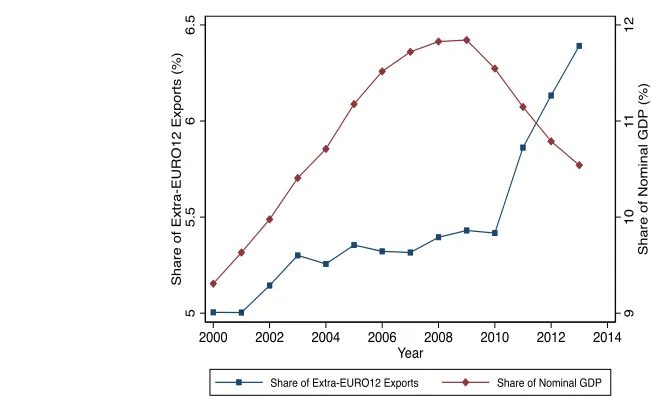
2008-2013 period, while real merchandise exports in the rest of the euro area increased by only 6.8% during the same years. As a result, and as shown in Figure 1, the share of euro area merchandise exports to non-euro area countries accounted for by Spain increased markedly during this period (especially in 2011-13), despite the contemporaneous decline in the relative weight of Spain’s GDP in the euro area’s GDP. Very similar patterns are observed for the cases of Portugal and Greece as well as for various other euro-area countries (see Appendix D.1).2
Figure 1: The Spanish Export Miracle
9 10 11 12 Sh a re o f N o mi n a l G D P (% ) 5 5.5 6 6.5 Sh a re o f Ext ra -EU R O 1 2 Exp o rt s (% )
2000 2002 2004 2006 2008 2010 2012 2014 Year
Share of Extra-EURO12 Exports Share of Nominal GDP
1The implied 6.9% annual growth in real exports from 2009 to 2013 almost doubled the 3.8% annual growth in real exports during the period 2000-2008.
At first glance, this remarkable export performance appears to be consistent with the goals of the type of “internal devaluation” processes advocated by international organizations (such as the IMF, the ECB or the European Commission) since the onset of the crisis. According to this thesis, wage moderation coupled with a set of structural reforms (most notably labor market reforms) led to a fall in relative unit labor costs, allowing Southern European firms to reduce their relative export prices and increase their market shares abroad. Nevertheless, in the Spanish case, the adjustment in labor costs achieved via these policies was modest up to 2013 and this channel is believed to have had a limited contribution to export growth over the period 2010-13 (see, for instance, IMF, 2015, 2018; Salas, 2018).
What explains then the remarkable export growth in Spain, Portugal and Greece over the period 2010-2013? At least for the case of Spain, an often-invoked alternative explanation relates the growth in exports directly to the collapse in domestic demand. According to this hypothesis, the unexpected demand-driven reduction in Spanish firms’ domestic sales, in combination with the irreversibility of certain investments in inputs, freed up capacity that these firms used to serve customers abroad.3 More precisely, this explanation posits that, as domestic demand dropped,
Spanish firms were able to cut their short-run marginal costs by reducing their usage of flexible inputs (e.g., temporary workers and materials) relative to their usage of fixed inputs (e.g., physical capital and permanent workers). This fall in short-run marginal costs translated into a gain in competitiveness in foreign markets and, consequently, to an increase in firms’ exports.4
This alternative explanation resonates with the “vent-for-surplus” theory of the benefits of international trade, which has a long tradition in economics dating back to Adam Smith.5 Despite
its intuitive nature and distinguished lineage, the link between a domestic slump and export growth is hard to reconcile with modern workhorse models of international trade. The reason for this is that these canonical models – including those emphasizing product differentiation and economies of scale as in Krugman (1984) and Melitz (2003) – assume that firms face constant marginal costs of production, an assumption that implies that demand shocks in one market do not affect a firm’s sales in another market.
In this paper, we leverage Spanish firm-level data from 2002 to 2013, and geographic variation 3See “La exportación como escape” in El País, 1/16/2016, for a journalistic account in Spanish with some specific case studies (https://elpais.com/economia/2016/01/14/actualidad/1452794395_894216.html). Further firm-level examples are provided in the more recent “El milagro exportador español” in El País, 5/27/2018 (http://elpais.com/economia/2018/05/25/actualidad/1527242520_600876.html), a newspaper article which was inspired by an early version of our paper.
4Generally, one can interpret this explanation as encompassing any mechanism that makes firms’ short-run marginal cost curves increasing and that, thus, links the drop in firms’ domestic demand to a downward move-ment along their supply curves. This effect is distinct from that of an “internal devaluation”, which is associated with a downwardshiftin firms’ marginal cost or supply curves (e.g., reductions in the price of factors or materials, or increases in productivity).
across Spanish regions in the reduction in domestic demand that took place during the Great Recession, to study the empirical relevance of the “vent-for-surplus” mechanism. To do so, we first divide our sample into a “boom” period (2002-08) and a “bust” period (2009-13), and measure the extent to which, at the firm level, a decline in the domestic sales in the bust period relative to the boom period is associated with an increase in export sales over the two periods. When measuring this association, we control for “boom-to-bust” changes in observed marginal cost shifters (i.e., measures of factor prices and productivity) to account for potential internal devaluation effects.
To further isolate demand-driven changes in domestic sales, we develop an instrumental vari-able approach that exploits the fact that the Great Recession affected different geographical areas in Spain differentially. In particular, we rely on municipality-level registration data on a major household durable consumption item, vehicles, as well as on municipality-to-municipality manu-facturing sales data (from tax records of firm-level sales within Spain) to construct an instrument proxying the extent to which the Great Recession affected the domestic demand faced by Spanish manufacturing firms located in different municipalities. More precisely, we employ the municipality-to-municipality trade flows to estimate the extent to which firms in a given municipality are exposed to demand shocks in other municipalities, and we use changes in the municipality-level stock of vehicles per capita between 2002-08 and 2009-13 as a proxy for the changes in demand in each municipality caused by the Great Recession.
To understand the properties of our estimates of the causal impact of demand-driven changes in domestic sales on exports, we first rely on a commonly used model of firms’ export behavior: a model à la Melitz (2003). For our purposes, this framework serves the role of identifying several empirical challenges that one encounters when measuring the relevance of the “vent-for-surplus” mechanism; i.e., when measuring the causal impact of changes in a firm’s domestic sales due to changes in its domestic demand on exports.6 We draw two main conclusions from our theoretical
analysis. First, as long as firms’ marginal cost shifters (i.e., firms’ productivity and production factor costs) are not perfectly observable – and their unobserved component is not fully captured by various fixed effects – there will tend to be apositivespurious correlation between domestic sales and exports that is not informative about the impact of demand-driven changes in the former on the latter. Second, an instrumental variable approach identifies the causal impact of demand-driven changes in domestic sales on exports as long as the instrument satisfies two conditions: (i) it is a good predictor of the domestic sales of Spanish firms, and (ii) it is not correlated with firms’ unobserved marginal cost or export-demand shifters.7
trade flows between any two Spanish municipalities. We compute these gravity-based estimates using municipality-to-municipality sales data; these estimates reveal a significant amount of “home bias” within Spain, with shipments declining in distance with an elasticity of around −0.4 even
after controlling for the discontinuity in sales observed when shipping outside a firm’s municipality. These results are consistent with the findings of Hillberry and Hummels (2008) for the U.S. and of Díaz-Lanchas et al. (2013) for Spain.8 To find a credible proxy for ‘local demand’, we invoke
an extensive literature in empirical macroeconomics documenting that consumption of durable goods such as vehicles is strongly procyclical (see, for instance, the survey by Stock and Watson, 1999). More recently, Mian et al. (2013), Hausman et al. (2019), and Waugh (2019) have also documented a strong link between wealth (or income) shocks and vehicle consumption. Against this backdrop, we use as an instrument for a firm’s to-bust change in domestic sales the boom-to-bust change in a weighted-sum of the stock of vehicles per capita in all municipalities other than the municipality in which the firm is located, with weights obtained from our gravity-equation estimation. Our first-stage results indicate that our instrument is indeed relevant.
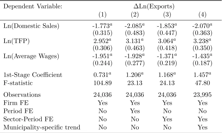
Armed with these first-stage results, we show that a largerdemand-drivendrop in domestic sales in the bust period relative to the boom period is associated with a significantly larger growth in export sales from boom to bust (conditional on exporting in both periods). Furthermore, these IV estimates are significantly larger than the OLS ones. This is consistent with the biases predicted by our baseline Melitz (2003)-type model in the plausible scenario in which our covariates only imperfectly control for a firm’s supply determinants. Specifically, our IV estimates point at an intensive-margin elasticity of exports to domestic sales in the neighborhood of−1.6, while the OLS
one is around −0.3. To assuage concerns about our long-differences approach to identification,
we also present estimates that break the period 2002-2013 into four subperiods (2002-05, 2006-08, 2009-11, 2012-13), and which allow for the inclusion of municipality-specific time trends in the estimation. This robustness exercise shows that our estimates are not biased by the presence of underlying heterogeneous trends across regions in Spain. When estimating the effect of a demand-driven changes in domestic sales on the probability of exporting, we instead find quantitatively small effects that are somewhat sensitive to the way in which the extensive margin of exporting is measured.
As indicated above, a potential challenge to our identification approach is that the boom-to-bust changes in our instrument may be correlated with the extent to which unobserved shifters of the firm’s marginal cost curve changed in the bust period relative to the boom period. Although we do not use information on demand changes in the firm’s own municipality when constructing the instrument, one may still be concerned about spatial correlation in demand shocks posing a threat to identification. With that in mind, in section6we provide additional pieces of evidence that are consistent with the empirical relevance of the “vent-for-surplus” hypothesis and that address some specific sources of endogeneity that could affect the validity of our baseline instrument.
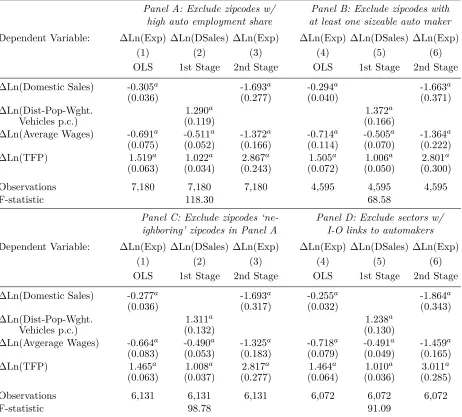
First, an identification threat arises if differences in the severity of the contraction in vehicle purchases across Spanish municipalities are not exclusively a reflection of differences in demand shocks, but also partly a reflection of unobserved production costs affecting car manufacturers. According to this hypothesis, if a significant share of vehicles is sold in the near vicinity of where they are produced, municipalities that concentrate a significant share of firms operating in the auto industry could observe a correlation in the boom-to-bust changes in production costs and nearby purchases of new vehicles. Our results are robust to this identification threat. Both the relevance of our instrument as well as the finding of a sizable negative elasticity between domestic sales and exports are robust to excluding from the estimating sample: (a) all firms in the auto industry, no matter where they are located; (b) all firms located in any zip code that hosts at least one auto-maker employing more than 20 workers; (c) all firms located in any zip code that is geographically close to a zip code in which a significant share of manufacturing employment is in the auto industry; and (d) all firms producing in sectors that are either leading input providers or leading buyers of the vehicles manufacturing industry.
Second, although we control for firm-specific average wages in all of our specifications, compo-sitional changes in the firm’s workforce may have caused changes in effective labor costs that our wage measure does not capture correctly. An important feature of the Spanish labor market is the division of the workforce into permanent and temporary workers, the latter group being typically less productive than the former (see Dolado et al., 2002). We do indeed observe that firms whose share of temporary workers dropped by more in the bust relative to the boom experienced a smaller drop in their exports, consistently with the hypothesis that an increase in the ratio of permanent to temporary workers had an effect equivalent to a positive supply shock. The elasticity of ex-ports with respect to domestic sales remains however largely unaffected when we control for the firm’s change in the share of temporary workers. Similarly, controlling for the change in financial costs experienced by exporters or for proxies of trade credit available to firms does not change the second-stage estimate of the elasticity of exports with respect to domestic sales. In addition, in section 6 we explore the robustness of our results to alternative constructions of our instrumental variable and to an alternative approach to measuring firm-level total factor productivity.9
though the statistical significance of this result is sensitive to which factors one classifies as “fixed”. Finally, we employ our model with increasing marginal costs and the corresponding IV esti-mates to quantitatively evaluate the importance of the “vent-for-surplus” mechanism in explain-ing the 2009-13 observed export miracle in Spain. More specifically, we implement a variance-decomposition exercise to determine the extent to which the domestic slump in Spain was driven by demand versus supply shocks. We then use our model to predict the boom-to-bust growth in Spanish exports that we would have observed if there had been no change in demand between the boom and bust periods. We find that, in this case, the growth in Spanish exports would have been 51.71% smaller than what we observe in the data and, thus, we conclude that slightly more than half of the Spanish export miracle of the period 2009-2013 can be attributed to the “vent-for-surplus” mechanism.
Our paper connects with several branches of the literature. As mentioned above, we relate the Spanish export miracle to Adam Smith’s “vent-for-surplus” theory. The international trade literature has largely ignored this hypothesis as exemplified by the fact that we have only found one mention (in Fisher and Kakkar, 2004) of the term “vent-for-surplus” in all issues of theJournal of International Economics.10 Nevertheless, there has been an active recent international trade
literature focused on relaxing the assumption of constant marginal costs in the canonical (Melitz) model of firm-level trade, and has shown that, in the presence of increasing marginal costs, there is a natural substitutability between domestic sales and exports for which there is supporting empirical evidence. This literature includes the work of Vannoorenberghe (2012), Blum, Claro and Horstman (2013), Soderbery (2014), and Ahn and McQuoid (2017). Relative to this prior literature, our paper exploits plausibly exogenous variation in demand during a particularly salient episode to identify the causal effect of a drop in domestic sales on exports. Additionally, it provides an approach to identify and structurally estimate the slope of firms’ short-run marginal cost curves. Relatedly, in contemporaneous work, Fan et al. (2018) exploit variation in the extent to which Chinese authorities enforce the collection of value-added taxes to establish a negative causal link between the profitability of domestic sales and firm-level exports. Conversely, using French data over the period 1995-2001, Berman et al. (2015) document a positive causal effect of changes in firm-level exports on firm-level domestic sales. Their identification strategy (based on exogenous variation in foreign demand conditions) is quite distinct from ours and so is their setting, since 1995-2001 was a tranquil period of sustained economic growth in France. In AppendixH.1, we use data on Spanish firms for the period 2002-07 to perform an analysis analogous to that in Berman et al. (2015), and we find no evidence supporting the positive causal relationship between exports and domestic sales that these authors previously found; on the contrary, for most specifications, we find a negative causal effect of (plausibly) exogenous changes in exports on domestic sales, in line with our core finding of substitution between exports and domestic sales.11
10A broader search to include top general-interest journals identified Neary and Schweinberger (1986), who provide a neoclassical rationale for the “vent-for-surplus” idea.
The rest of the paper is structured as follows. In section2, we lay out a baseline model of firm behavior in the spirit of Melitz (2003) and discuss its implications for the estimation of the causal impact of demand-driven changes in domestic sales on exports. In section 3, we introduce our firm-level data and, in section 4, we develop our core instrumental variable estimation approach. The results of this instrumental variable approach are presented in section5. We present additional evidence in favor of the “vent-for-surplus” mechanism in section 6. In section 7, we generalize the baseline model à la Melitz (2003) to allow for non-constant marginal costs, and use this framework to quantify the importance of the “vent-for-surplus” channel in linking the slump in domestic demand to the growth in Spanish exports. We offer some concluding remarks in section 8.
2 Benchmark Model: Estimation Guidelines
As indicated in the Introduction, we aim to estimate the causal impact of within-firm demand-driven changes in domestic sales on firm-level exports. To guide our empirical analysis and our choice of an adequate estimator, we first consider the implications for this question of a model of exporting with heterogeneous firms along the lines of Melitz (2003), which is the canonical model of firm-level exports in the recent international trade literature. This model features the standard assumption of constant marginal costs. After presenting our evidence contradictory with this assumption, in section 7we will develop an extension of this benchmark model that allows for non-constant marginal costs. Crucially, the lessons we learn in this section about the properties of different estimators will also apply in the more general model.
2.1 Benchmark Model: Estimating Equation
We index manufacturing firms producing in Spain by i, the sectors to which firms belong by s,
and the two potential markets in which they may sell byj ={d, x}, with ddenoting the domestic
market and x denoting the export market. In principle, both the domestic and export market are
an aggregate of several destinations, but due to data limitations, we focus in the main text on this dichotomous case (we develop a multi-destination extension of our model in Appendix E.2).
In any given period, firm ifaces the following isoelastic demand in marketj,
Qij =
Pij−σ
Psj1−σEsjξ
σ−1
ij , σ >1, (1)
where Qij denotes the number of units of output of firmi demanded in marketj if it sets a price
Pij,Psj is the sector sprice index in j,Esj is the total sectoral expenditure in marketj expressed
in units of the numeraire; andξij is a firm-market specific demand shifter.
Firm i’s total variable cost of producingQij units of output for market j is given by
cijQij with cij ≡τsj 1
ϕi
wherecij denotes the marginal cost to firmi of selling one unit of output in marketj,τsj denotes
an iceberg trade cost, ϕi denotes firmi’s productivity, and ωi is the firm-specific cost of a bundle
of inputs. Additionally, we assume that firm i needs to pay an exogenous fixed cost Fij to sell a
positive amount in market j.
Firm i chooses optimally the quantity offered in each market j, Qij, taking the price index,
Psj, and the size of the market, Esj, as given. As the marginal production cost is independent of
the firm’s total output and the per-market fixed costs are independent of the firm’s participation in other markets, the optimization problem of the firm is separable across markets. Specifically, conditional on selling to a market j, firm isolves the following optimization problem
max Qij
n
Q
σ−1
σ ij P
1−σ σ sj E
1
σ sjξ
σ−1
σ ij −τsj
1
ϕi
ωiQij o
,
and sales by firmito marketj are thus Rij =PijQij = κ((ξijϕi)/(τsjωi))σ−1EsjPsjσ−1, whereκ is
a function ofσ. For the case of exports (j=x), and taking logs, we can rewrite this expression as:
lnRix = lnκ+ (σ−1) (lnξix+ lnϕi−lnωi)−(σ−1) (lnτsx−lnPsx) + lnEsx. (3)
The bulk of our empirical analysis will compare firm-level export behavior in a bust period, relative to a boom period. With that in mind, and letting ∆ lnX denote the log change in the
cross-year average value of X from boom to bust, we can express the log change in exports from
boom to bust as
∆ lnRix = (σ−1) [∆ lnξix+ ∆ lnϕi−∆ lnωi]−(σ−1) (∆ lnτsx−∆ lnPsx) + ln ∆Esx. (4)
In order to transition to an estimating equation, we model the change in firm-specific foreign demand, productivity and cost levels as follows:
∆ ln(ξix) = ξsx+uξix,
∆ ln(ϕi) = ϕs+δϕ∆ ln(ϕ∗i) +u ϕ i,
∆ ln(ωi) = ωs+δω∆ ln(ωi∗) +uωi. (5)
Note that we are decomposing these terms into (i) a sector fixed effect, (ii) an observable part of these terms for the case of productivity (ϕ∗i) and for input bundle costs (ωi∗), and (iii) a residual
term. We can thus re-write equation (4) as:
∆ lnRix =γsx+ (σ−1)δϕ∆ ln(ϕ∗i)−(σ−1)δω∆ ln(ωi∗) +εix, (6)
whereγsx≡(σ−1) [ξsx+ϕs−ωs−lnτsx+ lnPsx] + lnEsx, and where
εix = (σ−1) [uξix+u ϕ
Following analogous steps as above, we derive an expression for the change in domestic sales:
∆ lnRid=γsd+ (σ−1)δϕ∆ ln(ϕ∗i)−(σ−1)δω∆ ln(ω∗i) +εid, (8)
whereγsd≡(σ−1) [ξsd+ϕs−ωs−lnτsd+ lnPsd] + lnEsd, and where
εid= (σ−1) [uξid+u ϕ i −u
ω
i]. (9)
We use equations (6) through (9) to generate predictions for the asymptotic properties of several estimators of the response of log exports to demand-driven changes in log domestic sales. The assumption of constant marginal costs implies that, according to this baseline model, the parameter of interest is zero: demand-driven changes inlnRid have no causal effect onlnRix. However, many
estimators of the impact of log domestic sales on log exports based on observational data will yield estimates that differ from zero, even in large samples. We discuss here the asymptotic properties of different OLS and IV estimators.
Consider first using OLS to estimate the parameters of the following regression, which includes the change in log domestic sales as an additional covariate in equation (6):
∆ lnRix =γsx+ (σ−1)δϕ∆ ln(ϕ∗i)−(σ−1)δω∆ ln(ω
∗
i) +β∆ lnRid+εix. (10)
From equations (7), (9), and (10), the probability limit of the OLS estimator of the coefficient on domestic sales can be written as
plim( ˆβOLS) =
cov(∆ lnRix,∆ lnRid)
var(∆ lnRid) =
cov(uξix+uϕi −uiω, uξid+uϕi −uωi)
var(uξid+uϕi −uωi) , (11)
where we denote by∆ lnX the residual of a regression of a variable ∆ lnX on a set of sector fixed
effects and the observable covariates ∆ lnϕ∗i, and ∆ lnωi∗.
We draw two main conclusions from equation (11). First, as long as changes in productivity and production factor costs are not perfectly observable – and their unobserved component is not fully captured by the sector fixed effects – there will be a positive correlation between changes in exports and changes in domestic sales. Intuitively, unobserved productivity or factor cost changes will affect sales in the same direction in all markets in which a firm sells. In large samples, this will leadβˆOLS
to be positive and, thus, to be biased upwards as an estimate of the causal impact of demand-driven changes in domestic sales on exports. Second, even when one proxies for changes in productivity and factor costs perfectly (i.e., uϕi = uωi = 0), in the presence of a non-zero correlation in the
change in residual demand faced by firms in domestic and foreign markets (i.e., cov(uξix, uξid)6= 0),
the estimatorβˆOLS will also converge to a non-zero value. As this residual demand does not capture
sector- and market-specific aggregate shocks (which are controlled by the sector fixed effects), it seems plausible thatuξix and uξid will be positively correlated in the data, leadingβˆOLS again to be
Consider next using an IV estimator of the parameters in equation (11). Specifically, consider instrumenting ∆ lnRid with an observed covariate Zid such that Zid is either a proxy for ∆ lnξid
or has a causal impact on this firm-specific domestic demand shifter. In this case, the probability limit of the IV estimator ofβ is
plim( ˆβIV) =
cov(∆ lnRix,Zid)
cov(∆ lnRid,Zid)
= cov(u ξ ix+u
ϕ
i −uωi,Zid)
cov(uξid+uϕi −uωi,Zid), (12)
where, as above, we use Zid to denote the residual from projecting Zid on a vector of sector fixed
effects and on the observable covariates ∆ lnϕ∗i, and ∆ lnωi∗. The constant-marginal-cost model
predicts thatβˆIV converges in probability to the true zero causal effect of demand-driven changes in
domestic sales on exports as long as the variableZidsatisfies two conditions: (a) it is correlated with
the change in domestic sales of firm iafter partialling out sector fixed effects as well as observable
determinants of the firm’s marginal cost; and (b) it is mean independent of the change in firm-specific unobserved productivity,uϕi, factor costs,uωi, and export demanduξix. As illustrated by the
second equality in equation (12), an instrument can only (generically) verify conditions (a) and (b) if its effect on domestic sales worksexclusively through the component of the change in domestic demand that is not accounted for by the sector fixed effects and the observable covariates included in the estimating equation, i.e., if it works exclusively throughuξid.
Although our discussion above has centered around the role of unobserved supply and export demand factors in biasing estimates of β, Berman et al. (2015) emphasize that measurement
error in both domestic sales and exports constitutes an additional source of possible bias when estimating the effect of exports on domestic sales (or vice versa). Because in many empirical settings – ours included – domestic sales are computed by subtracting exports from the total sales of firms, measurement error in firm total sales and exports will lead to a bias in the OLS estimate
ˆ
βOLS that is likely to be of the opposite sign to that generated by the unobserved supply and export
demand shocks accounted for by the residuals defined in equations (7) and (9). Consequently, as we detail in AppendixE.1(see also Berman et al., 2015), negative values ofβˆOLS in large samples
may be compatible with firms having constant marginal costs as long as the researcher’s measures of either total sales or exports are affected by measurement error. Nevertheless, as we also show in AppendixE.1, if an instrument satisfies the same conditions (a) and (b) outlined above, and is also mean independent of the measurement error in exports, the IV estimator in equation (12) will still converge to zero in the presence of measurement error in total sales and exports.12
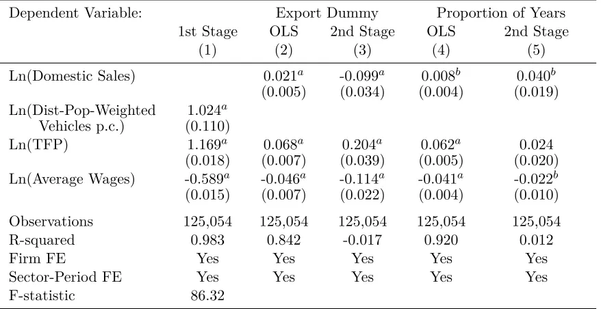
We have focused our discussion on the intensive margin of exports, namely the impact of domestic demand shocks on the level of exports conditional on exporting. In AppendixE.3, we show that an analysis of the extensive margin of exports modeled as a linear probability model delivers 12As mentioned above, in Appendix E.2, we generalize our model to incorporate multiple domestic and foreign markets. Theoretically, firms’ choice over multiple export destinations may render instruments Zidinvalid, even if
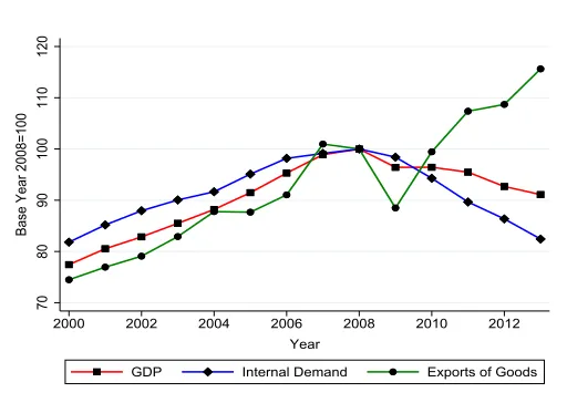
Figure 2: The Great Recession in Spain
70
80
90
100
110
120
Base Year 2008=100
2000 2002 2004 2006 2008 2010 2012
Year
GDP Internal Demand Exports of Goods
very similar insights. More specifically, when estimating the effect of demand-driven changes in domestic sales on the probability of exporting, even if the true effect were to be zero, one is likely to obtain a positive OLS estimate whenever productivity and production factor costs are not perfectly captured by sector fixed effects and observable controls, or whenever unobserved firm-specific demand shocks are positively correlated across the domestic and export markets. An instrument satisfying conditions (a) and (b) above will continue to effectively remove these biases as long as it satisfies the additional condition of being mean independent of the part of the change in the firm’s fixed cost of exporting not captured by sector fixed effects and marginal cost proxies (see Appendix E.3for more details).
3 Setting and Data
To construct a plausibly exogenous measure of the changes in domestic demand faced by firms, we exploit geographical variation in the severity of the impact of the Great Recession of the late 2000s and early 2010s in Spain. In this section, we describe the setting and data, and we defer a more detailed account of our identification strategy to section 4.
3.1 The Great Recession in Spain: Description
The macroeconomic history of Spain during the period 2000-2013 is a tale of a boom followed by a bust. As shown in Figure 2, between the year 2000 and the peak of the cycle in 2008, Spain’s GDP and internal demand grew by approximately 20% in real terms.13 In the five subsequent years
until 2013, domestic demand decreased to the level of the year 2000, while real GDP fell by an accumulated 8.9%. In that same period, the unemployment rate shot up from 9% to 26%.
that the economic boom of the early 2000s was primarily fueled by a real estate bubble. The construction sector accumulated an increasing share of GDP and employment.14 For instance, in
2006, 658,000 new houses were built in Spain, a number corresponding to 80% of those built in Germany, Italy and the UKcombined.15 This real estate boom was in turn fostered by the increased
availability of cheap credit to households, firms and real estate developers, which resulted from capital inflows related to the adoption of the euro in 2002 and the global savings glut (Santos, 2014). As a result, the ratio of mortgage credit to GDP went up from 40% in 2000 to 100% in 2008 (Basco and Lopez-Rodriguez, 2018). Importantly, the very high loan-to-value (LTV) ratios associated with residential mortgage credit were partly used by households to finance private consumption, particularly vehicle purchases (Masier and Villanueva, 2011).
The unraveling of the subprime mortgage market in the U.S. in the summer of 2007 had an immediate effect on the supply of credit in Spain. However, the effects were fully transmitted to the real economy only about one year later, coinciding with the fall of Lehman Brothers in September 2008, and the sudden stop in capital inflows (Basco and Lopez-Rodriguez, 2018). The recession officially started in the fourth quarter of 2008, and intensified during 2009 with a 3.6% annual drop in real GDP. The growth in the stock of vehicles in Spain, which had been stable at an average rate of 3.6% a year during the boom, suddenly came to a halt in 2008 (see FigureC.1in Appendix
C). In fact, in 2013, the national stock of vehicles per capita in Spain waslower than in 2008 by around 52,000 units.
Importantly for the identification strategy we describe in the next section, the real estate boom and subsequent bust featured significant geographic variation, affecting mainly some parts of the Mediterranean coast and medium-sized and large cities. As we shall document in section 4, this in turn translated into substantial geographic variation in the extent to which the Great Recession affected domestic demand and thus the domestic sales of Spanish firms.
3.2 The Spanish Export Miracle
As Figure 2 illustrates, the evolution of Spain’s aggregate merchandise exports during the period 2008-2013 was significantly different from that of aggregate domestic demand. After a significant 11.5% drop in real terms during the global trade collapse of 2008-09, aggregate exports grew during the period 2009-2013 at an even faster rate than during the boom years. Specifically, while exports had grown by an accumulated 34% in the eight-year period 2000-2008, they grew by a very similar 31% in just the four years between 2009 and 2013. This acceleration in export growth occurred at a time during which all indicators of domestic economic activity were showing a significant decline. As a consequence, the fall in real GDP was significantly smaller than the fall in domestic demand, and the ratio of exports of goods to GDP grew from 15.1% in 2009 to 23.33% in 2013. In Appendix
D.2, we use the firms in our sample to describe the dynamics of the exports-to-sales ratio by sector. 14The share of total employment in the construction sector peaked at 13.5% in the summer of 2007 and then collapsed, reaching 5.4% by early 2014, with a similar pattern for the contribution of this sector to Spain’s GDP (12.4% in 2007 and 6.8% in 2014).
One might wonder whether a depreciation in the euro could explain the growth in Spanish exports during the period 2009-2013. Figure1in the Introduction shows however that this could not have been the main explanation, as Spanish exports to non-euro area countries clearly outperformed those of other countries in the euro area (even though Spain’s GDP dropped faster than the euro area average).16 It has also been argued that Spain underwent an internal devaluation during this
period (through wage moderation starting in 2009, and via a labor market reform in 2012), but there is little evidence that these policies had a significant effect on relative production costs before 2012. For instance, unit labor costs in Spain were only 2.2% lower in 2012 than in their peak in 2009 (OECD Statistics). Conversely, as we document in Appendix D.3, export prices (unit values from product-level export data) in Spanish manufacturing fell relative to export prices in other euro area countries from the onset of the crisis, before Spanish unit labor costs had started to fall. Motivated by these facts, we will hereafter focus on an exploration of the “vent-for-surplus” mechanism, according to which the domestic slump, by freeing up production capacity, might have directly incentivized Spanish producers to sell their goods in foreign markets. More precisely, we hypothesize that the domestic slump led firms to move down along their short-run marginal-cost schedule, thereby allowing them to lower their export prices and gain market share in export markets.17
In principle, the associated growth in exports could have materialized along the intensive margin (with continuing exporters increasing their exports) or along the extensive margin (via net entry into the export market). Later in the paper, we will explore both margins, but descriptive evidence suggests that the bulk of the growth was driven by the intensive margin. Using detailed Spanish Customs data, De Lucio et al. (2017a) find that net firm entry (i.e., new exporters net of firms quitting exporting) contributed a mere 14% to the export growth between 2008 and 2013, while the remaining 86% was driven by continuing exporters. Similarly, in our sample of manufacturing firms, we find that continuers contributed 91% of the growth in exports between the boom and the bust periods, and the extensive margin only accounted for 9% of export growth.18
3.3 Data Sources
Our data cover the period 2000-2013 and come from various confidential administrative data sources. The first is the Commercial Registry (Registro Mercantil Central). It contains the an-nual financial statements of around 85% of registered firms in the non-financial market economy in 16An interesting aspect of Figure1is that most of therelativetake-off of Spain occurred after 2010. The same is not true when looking at Spain’s share in overall goods exports (including exports to euro area countries); in that case, Spain’s share increased markedly already in 2009. This suggests that the increase in Spanish exports (relative to euro area countries) immediately following the Great Recession was largely driven by increased exports within the EU zone.
Spain.19 Among other variables, it includes information on the following: sector of activity (4-digit
NACE Rev. 2 code), 5-digit zip code of location, net operating revenue, material expenditures (cost of all raw materials and services purchased by the firm in the production process), labor ex-penditures (total wage bill, including social security contributions), number of employees (full-time equivalent), and total fixed assets.20
The second dataset is the foreign transactions registry collected by the Bank of Spain (Banco de España). For both exports and imports, it contains transaction-level information on the fiscal identifier of the Spanish firm involved in the transaction, the amount transacted, the product code (SITC Rev. 4), the country of the foreign client, and the exact date of the operation (no matter when the payment was performed). Starting in 2008, however, the dataset’s information on the product code and on the destination country became unreliable. The reason for this is that, to save on administrative costs, the entities reporting to the Bank of Spain were given the option of bundling a set of transactions together. In those cases, each entry reflects only the country of destination and product code of the largest transaction in that bundle (see Appendix B for more details). This feature of the dataset precludes us from studying exports at the firm-product-destination-year level during the crisis, but we can still reliably aggregate this transaction-level data to obtain information on total export volume by firm and year.
This international trade database has an administrative nature becauseBanco de Españalegally required financial institutions and external (large) operators to report this information for foreign transactions above a fixed monetary threshold. Until 2007, the minimum reporting threshold was fixed at 12,500 euros per transaction. Since 2008 until the end of the mandatory registry in 2013, information had to be reported for all transactions performed by a firm during a natural year as long as at least one of these transactions exceeded 50,000 euros. In order to homogenize the sample, for the period 2000 to 2007, we only record a positive export flow in a given year for firms that had at least one transaction exceeding 50,000 euros in that year (for more details see AppendixB). The foreign transactions registry collected by the Bank of Spain was discontinued in early 2014, which precludes us from extending our analysis past the year 2013.
In both datasets, a firm is defined as a business constituted in the form of a Corporation (Sociedad Anónima), a Limited Liability Company (Sociedad Limitada), or a Cooperative ( Cooper-ativa). We merge both datasets using the fiscal identifier of each firm. Using the merged database, we define each firm’s domestic sales as the difference between its total annual sales and its total export volume (see section 2 and Appendix E.1 for a discussion of measurement error in these variables).
19We obtain information on the Commercial Registry from two different sources: (i) the Central de Balances dataset, compiled by the Bank of Spain, and (ii) theSabi dataset, compiled by Informa (a private company). For details on how we combine these two datasets, see Almunia et al. (2018).
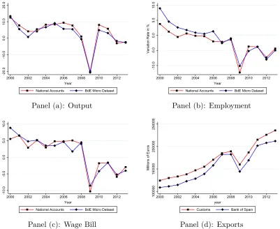
Figure 3: Output, Employment, Wage Bill and Export Dynamics
20.0
10.0
0.0
-10.0
-20.0
Variation Rate in %
2000 2002 2004 2006 2008 2010 2012
Year
National Accounts BdE Micro Dataset
Panel (a): Output
10.0
5.0
0.0
-5.0
-10.0
Variation Rate in %
2000 2002 2004 2006 2008 2010 2012
Year
National Accounts BdE Micro Dataset
Panel (b): Employment
10.0
5.0
0.0
-5.0
-10.0
Variation Rate in %
2000 2002 2004 2006 2008 2010 2012
Year
National Accounts BdE Micro Dataset
Panel (c): Wage Bill
100000
150000
200000
250000
Millions of Euros
2000 2002 2004 2006 2008 2010 2012
year
Customs Bank of Spain
Panel (d): Exports
To confirm the validity of the information contained in the resulting dataset, we compare its coverage with the official publicly available aggregate data on output, employment and total wage bill (from National Accounts) and on goods exports (from Customs). Figure 3 shows that our dataset tracks nearly perfectly the aggregate evolution over time of output, employment, total payments to labor, and exports. Due to the reporting thresholds described above, aggregate exports in our sample naturally fall a bit short of aggregate exports in the Customs data, but note that the gap is very similar in the boom and bust periods (the average coverage is91.8%in 2000-08 and 91.3%in 2009-13).21
the Spanish National Statistical Office (Instituto Nacional de Estadística). When matching this municipality-level data with our firm-level data, we need to deal with the fact that the information on the location of firms is provided at the zip code level, and that the mapping between munic-ipalities and zip codes is not one-to-one. More precisely, larger municmunic-ipalities are often assigned multiple zip codes and, in a very small number of cases, a single zip code is assigned to more than one municipality. In the former case, we associate the same value for the stock of vehicles per capita to all firms located in the same municipality, independently of the zip code of location; for firms in zip codes containing multiple municipalities, we associate with them a stock of vehicles per capita constructed as an average the stock of vehicles per capita across these municipalities.
We also employ data on firm-level sales within Spain.22 We obtained this data from the Spanish
Tax Agency (Agencia Estatal de Administración Tributaria, AEAT), which collects this data from all firms (legal entities) and professionals (natural persons) that undertake economic activities in Spain (see more details in Appendix B). The AEAT was willing to share one year of data with us, so we work with data for the year 2006 because it is the first year for which a comprehensive digitization of the data is available. We obtained two datasets from the AEAT: first, aggregate data on municipality-to-municipality flows for all firms in the manufacturing sector, excluding sales of entitites in the auto industry; and second, firm-to-municipality sales for those manufacturing firms that exported in the boom as well as in the bust.
When exploring the robustness of our results, we use information on additional variables. The underlying sources for these variables are discussed in AppendixB.
4 Identification Approach
In this section, we first describe our identification approach, and later highlight various potential threats affecting this strategy and how we seek to address them.
4.1 A Geography-based Proxy of Demand Changes
As explained in section3.1, a key characteristic of the Great Recession in Spain is that it affected different regions differently. Panel (a) in Figure4illustrates this fact. The figure plots the standard-ized percentage change in domestic sales for the average manufacturing firm located in each of the 47 Spanish peninsular provinces and operating in at least one year of the boom period (2002-2008) and at least one year of the bust period (2009-2013).23 The provinces where the average firm
experienced a reduction in domestic sales smaller than the national average are in darker color, while those where the average firm experienced a larger reduction in domestic sales are in lighter color. Specifically, Figure4 illustrates that firms located in the Northern and Western regions saw
22We thank Francesco Serti for having brought to our attention the existence of these data.
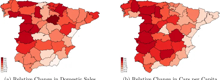
Figure 4: The Great Recession in Spain: Variation Across Provinces
(a) Relative Change in Domestic Sales (b) Relative Change in Cars per Capita Notes: For each province, panel (a) illustrates the standardized percentage change in average firm-level domestic sales between the period 2002-2008 and the period 2009-2013, where the average is computed across manufacturing firms active in at least one year in both periods. Therefore, if this variable takes valuepfor a given province, it
means that the average firm located in this province experienced a relative change in average yearly domestic sales between 2002-2008 and 2009-2013 that waspstandard deviations above the change experienced by the average
province. Panel (b) illustrates the standardized percentage change in vehicles per capita between the period 2002-2008 and the period 2009-2013. Therefore, if this variable takes valuepfor a given province, it means that
this province experienced a relative change in vehicles per capita between 2002-2008 and 2009-2013 that wasp
standard deviations above the change experienced by the average province.
changes in domestic sales larger (less negative) than the average, while firms located in the center of the country and in Southern and Eastern regions experienced relatively large domestic sales reductions. Furthermore, deviations from the national average are sizable in many cases.
The heterogeneity in the changes in domestic sales that we document in panel (a) of Figure 4
could have been caused by heterogeneity in supply factors or by heterogeneity in factors affecting local demand for manufacturing goods. We next propose an approach to measuring variation in local demand for manufacturing goods.
Our approach consists in proxying changes in local demand for manufacturing goods using observed changes in demand per capita for one particular type of manufacturing products: vehicles. Panel (b) in Figure4shows that there is substantial variation in the degree to which the number of vehicles per capita changed across provinces between the boom and the bust years.24 Specifically,
the provinces in the Northwest and in the Southwest experienced a relative increase in the number of vehicles per capita, while the region around Madrid and the provinces in the Northeast and along the Mediterranean coast experienced a relative reduction. As in panel (a) of Figure4, the regional deviations from the national averages in panel (b) are large for many provinces.
domestic sales and in the boom-to-bust changes in the number of vehicles per capita. We illustrate this variation in Figure C.3 (see AppendixC.3) for the case of the two most populated provinces in Spain: Madrid and Barcelona.
Our core empirical strategy exploits the variation illustrated in Figures 4 and C.3 to identify the impact of domestic demand shocks on firms’ exports operating through its effect on the firms’ domestic (Spain-wide) sales. Specifically, we divide our sample into a “boom” period (2002-08) and a “bust” period (2009-13), and assess the extent to which a demand-driven decline in a firm’s domestic sales in the bust period relative to the boom period is associated with a relative increase in its export sales between these two periods. We choose this ‘long-differences’ approach to avoid having to take a stance on the precise lag structure of the effect of domestic demand on exports, and also because the macroeconomic evidence in Figure3 and the time series of the national stock of vehicles per capita in FigureC.1cleanly identify the year 2009 as the break between two distinct periods. Having said this, we will demonstrate in section6that our results are quantitatively robust to other classifications of the boom and the bust periods, and also remain qualitatively similar when breaking the sample into four subperiods (2002-05, 2006-08, 2009-11, 2012-13).
To build a measure of the boom-to-bust change in domestic demand for each Spanish firm, we follow a two-step procedure. First, we use observed boom-to-bust changes in the stock of vehicles per capita at the municipality level as a proxy for the boom-to-bust changes in the demand for manufacturing goods in those municipalities. For this, we rely on a body of work documenting that durable goods consumption, and vehicle purchases in particular, are strongly procyclical and thus are a useful proxy for changes in ‘local demand’, i.e., the overall propensity of an area’s inhabitants to consume (see Stock and Watson, 1999). Consistent with this notion, Mian et al. (2013) document how variation in the extent to which the U.S. subprime mortgage default crisis of 2007-10 affected household housing wealth in different areas in the United States translated into geographical variation in vehicle purchases.25 There is also a broader literature documenting the
large impact that housing wealth effects had on consumption more generally in the years around the Great Recession; e.g., Guren et al. (2020), Kaplan et al. (2020).
log population and log distance to back out the relevant weights needed to construct our baseline measure of firm-level exposure to local shocks. As a robustness check, we also exploit below our information on firm-level sales across destinations within Spain to estimate firm-to-municipality gravity equations and compute an alternative set of weights.
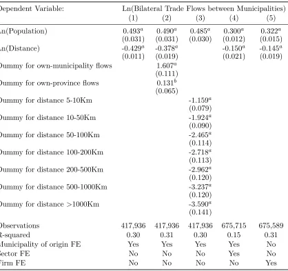
Estimates of this municipality-to-municipality gravity equation for Spanish manufacturing flows in the year 2006 are presented in columns 1 through 3 of Table1. The first column presents a par-simonious specification with municipality of origin fixed effects, log population of the municipality of origin, and log distance between origin and destination. The results illustrate the relevance of gravity forces, with shipments declining with distance with an elasticity of −0.429. The inclusion
in column 2 of dummies for own-municipality and own-province flows slightly reduces this distance elasticity, while these two dummies appear to have themselves a positive and significant effect on shipments. This suggests that part of the negative effect of distance on within-Spain municipality-to-municipality shipments is related to a discontinuous fall in shipments at the municipality border and at the province border. The extent of “home bias” at the municipality level is remarkably large: it implies that, ceteris paribus, shipments are exp(1.607) ≈5 times larger within a
munic-ipality than outside. The existence of such strong local home bias is in line with the findings of Hillbery and Hummels (2008) for the U.S., although the magnitude of this home bias is larger in our setting.26 Column 3 presents estimates for a third specification analogous to that in column
1 but employing a set of distance dummies to capture the effect of distance on sales. The results corroborate the fact that, controlling for municipality of origin fixed effects and for the population of the municipality of destination, sales decay monotonically with distance.
We combine the estimates in Table 1 with data both on the distance between any two munic-ipalities i and j and on the population of each possible municipality of destination j to predict
the share of domestic (within-Spain) sales that any firm located in municipality iwill sell in
mu-nicipality j. We use these shares to compute, for each municipality of origini, a weighted sum of
the local demand level (i.e., vehicles per capita) in all destinations j other than i. We do so for
the boom and for the bust periods (taking the average number of vehicles per capita within each period as our period-specific measure of demand in each municipality) and then we take the log difference of these period-specific average demand levels as our proxy for the demand shock that manufacturing firms located in any municipality i experienced between the boom and the bust
Table 1: Estimates from Gravity Equations at Municipal Level
Dependent Variable: Ln(Bilateral Trade Flows between Municipalities)
(1) (2) (3) (4) (5)
Ln(Population) 0.493a 0.490a 0.485a 0.300a 0.322a
(0.031) (0.031) (0.030) (0.012) (0.015)
Ln(Distance) -0.429a -0.378a -0.150a -0.145a
(0.011) (0.019) (0.021) (0.019) Dummy for own-municipality flows 1.607a
(0.111) Dummy for own-province flows 0.131b
(0.065)
Dummy for distance 5-10Km -1.159a
(0.079)
Dummy for distance 10-50Km -1.924a
(0.090)
Dummy for distance 50-100Km -2.465a
(0.114)
Dummy for distance 100-200Km -2.718a
(0.113)
Dummy for distance 200-500Km -2.962a
(0.120) Dummy for distance 500-1000Km -3.237a
(0.120) Dummy for distance>1000Km -3.590a
(0.141)
Observations 417,936 417,936 417,936 675,715 675,589
R-squared 0.30 0.31 0.30 0.15 0.31
Municipality of origin FE Yes Yes Yes Yes No
Sector FE No No No Yes No
Firm FE No No No No Yes
Note: a denotes 1% significance,b denotes 5% significance,c denotes 10% significance. Standard errors
clustered at the province (of origin) level are reported in parenthesis. The data on municipality-level trade flows for manufacturing firms is for the 2006 fiscal year. Ln(Population) denotes the log of the population of the destination municipality in 2006. Ln(Distance) denotes the log of the distance, in kilometers, between the two municipalities in each pair. The estimates in columns 1 to 3 use municipality-to-municipality sales data; the estimates in columns 4 and 5 use firm-municipality-to-municipality data.
shocks described here will play the role of the instrumentZid introduced in section 2.1. 27
destination level shipments within Spain for a sample of around 8,000 continuing exporters (i.e.,
firms that exported both in the boom as well as in the bust). We use this data in columns 4 and 5 of Table 1 to run gravity equations at the firm-destination level. For simplicity, we focus in column 4 on the parsimonious specification in column 1, extended in column 5 to account for firm fixed effects. The results are in line with those in column 1, but with somewhat smaller log population and log distance coefficients, as one would expect given that these specifications do not account for extensive margin variation in the set of municipalities firms sell to. As a robustness check, we present in section6.3results that rely on instruments analogous to that described above, but built using predicted sales shares based on the estimates of these firm-to-municipality gravity specifications.28
4.2 Threats to Validity of the Instrument
The main concern with our identification approach is that our municipality-level measure of demand changes between boom and bust might be correlated with changes in supply shocks affecting the firms located in the corresponding municipalities. This exclusion restriction is central to the validity of our strategy, so we next outline how it might be violated and how we deal with these potential threats to identification.
First, we control in our specifications for sector fixed effects. Thus, we base our identification on observing how domestic sales and exports changed between the boom and the bust for different firms operating in the same sector but located in regions experiencing different exposure to local demand changes. More specifically, by controlling for sector fixed effects we control for sector-specific foreign demand shocks, sector-specific trade cost shocks, and domestic supply shocks affecting Spanish firms (see definition of γsx in equation (6)). For example, these sector fixed effects control for shocks
such as the expiration of the Multi Fiber Arrangement on January 1, 2005, which eliminated all European Union quotas for textiles imported from China and which increased the competition that Spanish textile manufacturers faced both in the domestic and foreign markets.29
Admittedly, sector fixed effects may not effectively control for all heterogeneity across firms in their export demand shocks; specifically, firms located in different Spanish regions may be differentially affected by export demand shocks even if they operate in the same sector. A possible source of this heterogeneity in demand shocks is the different exposure of firms located in different Spanish regions to changes in demand in different foreign countries (e.g., firms located in Southern regions are more exposed to demand changes in Northern African countries than firms located in the north of Spain); in AppendixE.4, we provide suggestive evidence that this type of heterogeneity in export demand shocks is not, in practice, damaging for our instrument.
28We have also estimated gravity equations that use the firm-to-destination data and that include the border and distance dummies introduced in columns 2 and 3. Notably, we again find a remarkably large coefficient of 1.308 for the own-municipality dummy variable.
Second, as different firms operating in the same sector may experience different supply shocks, we also control for firm-specific measures of productivity and labor costs. By controlling for changes in wages and productivity at the firm level, we aim to identify the effect that changes in local demand had on firms’ exports through channels other than the internal devaluation channel. More specifically, these controls help address the concern that the reduction in unit labor costs observed in Spain during the period 2009-13 might have been heterogeneous across different Spanish regions in a manner that is correlated with our demand measure.
Our third approach to assuage endogeneity concerns is motivated by the fact that our various fixed effects and proxies for firm-level productivity and wage costs might not perfectly capture supply-side factors, and that unobservedresidual supply shocks might be correlated with our proxy for changes in local demand. For instance, this will be the case if changes in the stock of vehicles per capita in a municipality are not entirely due to changes in the supply of credit to households but also partly due to supply shocks affecting either the firms located in such municipality or in neighboring municipalities. This would be the case if these supply shocks (e.g., changes in labor payments not properly controlled for by our measure of firm-level wages) impact the purchasing power of consumers living in the corresponding municipalities. To deal with this threat to identification, in all regressions presented in this paper, we do not use information on the change in the number of vehicles per capita in the municipality of location of a firm when constructing our baseline instrument, which is thus a weighted sum of demand levels in municipalities other than the one where the firm is located. In section 6, we also present estimates from regression specifications in which we control for additional measures of municipality-specific boom-to-bust changes in economic conditions (e.g., changes in financial costs, changes in the share of temporary workers, etc.).
Finally, it is important to remark that, as illustrated in equation (12), any unobserved factor costs that are negatively correlated with our instrument will cause our IV estimator to be posi-tively biased. For example, if the tightening of the credit supply in a region caused firms’ marginal production costs to increase and consumers’ demand to fall, the resulting endogeneity of our in-strument would bias our IV estimator upwards. Thus, negative IV estimates of the elasticity of firm-level exports with respect to a firm’s domestic sales would still reflect patterns in the data that would be inconsistent with the constant marginal cost model described in section2.
5 Baseline Results
In this section, we present our baseline results on the impact of demand-driven changes in domestic sales on firms’ behavior in the export market. Specifically, in section 5.1, we present evidence on the impact of the Great Recession on Spanish firms’ intensive margin of exports. In section5.2, we present analogous evidence of its impact on the extensive margin.
5.1 Intensive Margin
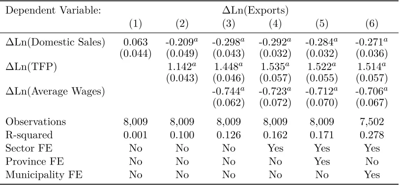
Table 2 presents OLS estimates of the elasticity of boom-to-bust changes in firms’ export flows with respect to boom-to-bust changes in domestic sales for continuing exporters – i.e., firms that exported both in the boom as well as in the bust. There are 8,009such firms in our dataset.
As discussed in section 2, when no instrument for the change in domestic sales is used in the estimation, even in a model with constant marginal costs, unobserved (residual) supply factors tend to make the OLS estimate of a firm’s change in foreign sales on its change in domestic sales positive. Conversely, measurement error in both total sales and exports tends to make this OLS estimate negative. As illustrated in column 1 of Table 2, when no controls are included, we estimate an OLS elasticity of export flows with respect to domestic sales that is very close to zero. Consistently with the expected biases in the OLS estimator, as we control for various sources of marginal cost heterogeneity across firms in the remaining columns of Table2, the OLS estimates become negative. Specifically, we control in column 2 for the change in firms’ productivity (estimated following the procedure in Gandhi et al., 2016, as detailed in Appendix F), and in column 3 for the change in the firm’s average wages (reported by the firm in its financial statement). Consistent with the discussion in section 2, controlling for these supply shocks reduces the OLS estimate of the coefficient on domestic sales. In fact, the coefficient turns negative (−0.298), indicating that, once
Table 2: Intensive Margin: Ordinary Least Squares Estimates
Dependent Variable: ∆Ln(Exports)
(1) (2) (3) (4) (5) (6)
∆Ln(Domestic Sales) 0.063 -0.209a -0.298a -0.292a -0.284a -0.271a
(0.044) (0.049) (0.043) (0.032) (0.032) (0.036)
∆Ln(TFP) 1.142a 1.448a 1.535a 1.522a 1.514a
(0.043) (0.046) (0.057) (0.055) (0.057)
∆Ln(Average Wages) -0.744a -0.723a -0.712a -0.706a
(0.062) (0.072) (0.070) (0.067) Observations 8,009 8,009 8,009 8,009 8,009 7,502
R-squared 0.001 0.100 0.126 0.162 0.171 0.278
Sector FE No No No Yes Yes Yes
Province FE No No No No Yes No
Municipality FE No No No No No Yes
Notes: a denotes 1% significance,bdenotes 5% significance,cdenotes 10% significance. Standard
errors clustered at the province level are reported in parenthesis. For any X, ∆Ln(X) is the
difference in Ln(X) between its average in the 2009-2013 period and its average in the 2002-2008
period. The estimation sample includes all firms exporting in at least one year in the period 2002-2008 and in the period 2009-2013.
associated with close to a0.3%increase in its overall export flows.
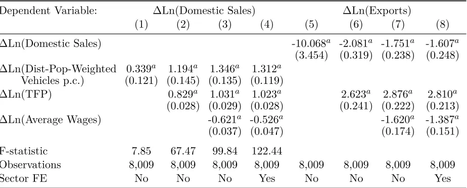
In Table3, we turn to our baseline two-stage least squares (TSLS) estimates of the elasticity of the firm’s boom-to-bust change in exports with respect to its boom-to-bust demand-driven change in domestic sales. As discussed in section2, if the instrument is orthogonal to both unobserved supply factors and to the measurement error in both total sales and exports, the corresponding TSLS estimator should converge to zero in large sample, as long as firms’ marginal costs are constant. The first-stage estimates (reported in columns 1 to 4 and plotted in panel (a) of Appendix Figure
C.4) reveal that firms located in municipalities that experienced a larger drop in the distance- and population-weighted municipality-level stock of vehicles per capita also suffered a larger decline in their domestic (Spain-wide) sales. This relationship is robust to controlling for our measures of firms’ changes in productivity and labor costs and for sector and province fixed effects: the statistic of anF-test for the null hypothesis that the change in the municipality-specific average of the stock
of vehicles per capita across all other municipalities that we use as our instrument has no impact on the domestic sales of the firms located in that municipality is in all specifications above threshold values generally applied to detect weak instrument problems, the only exception being the value of
7.85 in column 1.
The second-stage estimates (reported in columns 5 to 8) reveal elasticities of exports with respect to domestic sales that are significantly larger (in absolute value) than the OLS elasticities reported in Table 2.30 This is true regardless of whether one controls for sector and province
Table 3: Intensive Margin: Two-Stage Least Squares Estimates
Dependent Variable: ∆Ln(Domestic Sales) ∆Ln(Exports)
(1) (2) (3) (4) (5) (6) (7) (8)
∆Ln(Domestic Sales) -10.068a -2.081a -1.751a -1.607a
(3.454) (0.319) (0.238) (0.248)
∆Ln(Dist-Pop-Weighted 0.339a 1.194a 1.346a 1.312a
Vehicles p.c.) (0.121) (0.145) (0.135) (0.119)
∆Ln(TFP) 0.829a 1.031a 1.023a 2.623a 2.876a 2.810a
(0.028) (0.029) (0.028) (0.241) (0.222) (0.213)
∆Ln(Average Wages) -0.621a -0.526a -1.620a -1.387a
(0.037) (0.047) (0.174) (0.151) F-statistic 7.85 67.47 99.84 122.44
Observations 8,009 8,009 8,009 8,009 8,009 8,009 8,009 8,009
Sector FE No No No Yes No No No Yes
Note: a denotes 1% significance,b denotes 5% significance,cdenotes 10% significance. Standard errors clustered
by province appear in parenthesis. For anyX,∆Ln(X) is the log difference between the average ofX in 2009-2013
and its average in 2002-2008. ∆Ln(Dist-Pop-Weighted vehicles p.c.) is the instrument constructed using data on vehicles per capita at the municipal level and applying the weights from the gravity equation reported in column 1 of Table1. Columns 1-4 contain first-stage estimates; columns 5-8 contain second-stage estimates. F-statistic denotes the corresponding test statistic for the null hypothesis that the coefficient on Ln(Dist-Pop-Weighted Vehicles p.c.) equals zero.
preferred estimate in column 8 indicates an elasticity of exports with respect to domestic sales of around −1.6.31 It is clear that this elasticity is significantly more negative than the OLS one,
which we take to be a validation of the hypothesis, formalized in equation (11), that, even after controlling for sector fixed effects and for firm proxies of productivity and average labor costs, there still remains substantial unobserved determinants of firms’ marginal costs that induce a spurious positive correlation between their sales in the domestic and foreign markets. Also, the threats to the internal validity of the instrument notwithstanding (see section 4.2 for a detailed account of these threats), the fact that the TSLS estimate is negative is suggestive of the firm’s marginal cost function not being flat.
One might be concerned that, because firms’ total sales are a key input in the computation of our TFP measure, our empirical results are just unveiling a mechanical negative correlation between exports and domestic sales once one holds total sales revenue constant (by controlling for it). Although log TFP and log total sales are obviously positively correlated (as one would expect in light of our model), the correlation is far from perfect, particularly when considering log changes in these variables. More specifically, the correlation between log changes in TFP and log changes in total sales in data is 0.31 at the yearly level, while it is 0.56 when looking at boom-to-bust
‘long differences’ in these variables. To further assuage this concern, in section6.4 we explore the robustness of our results to an alternative measure of log firm TFP computed using value-added that features a much lower correlation with log firm sales.